Establishment of the Predicting Models of the Dyeing Effect in Supercritical Carbon Dioxide Based on the Generalized Regression Neural Network and Back Propagation Neural Network


Abstract
:
1. Introduction
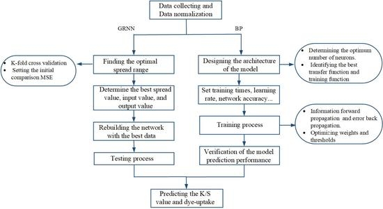
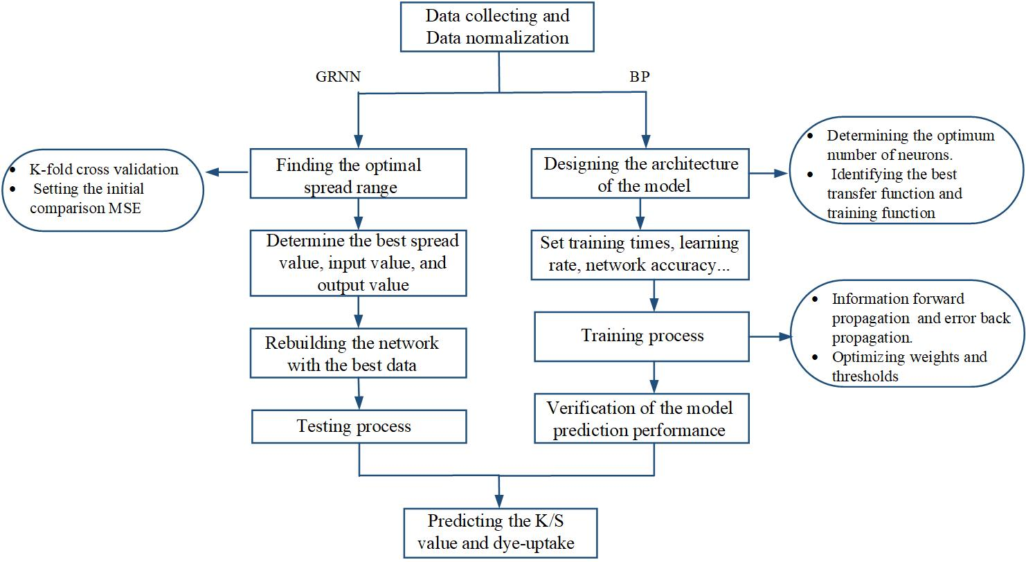
2. Methodology
2.1. Data Collection and Pre-Processing
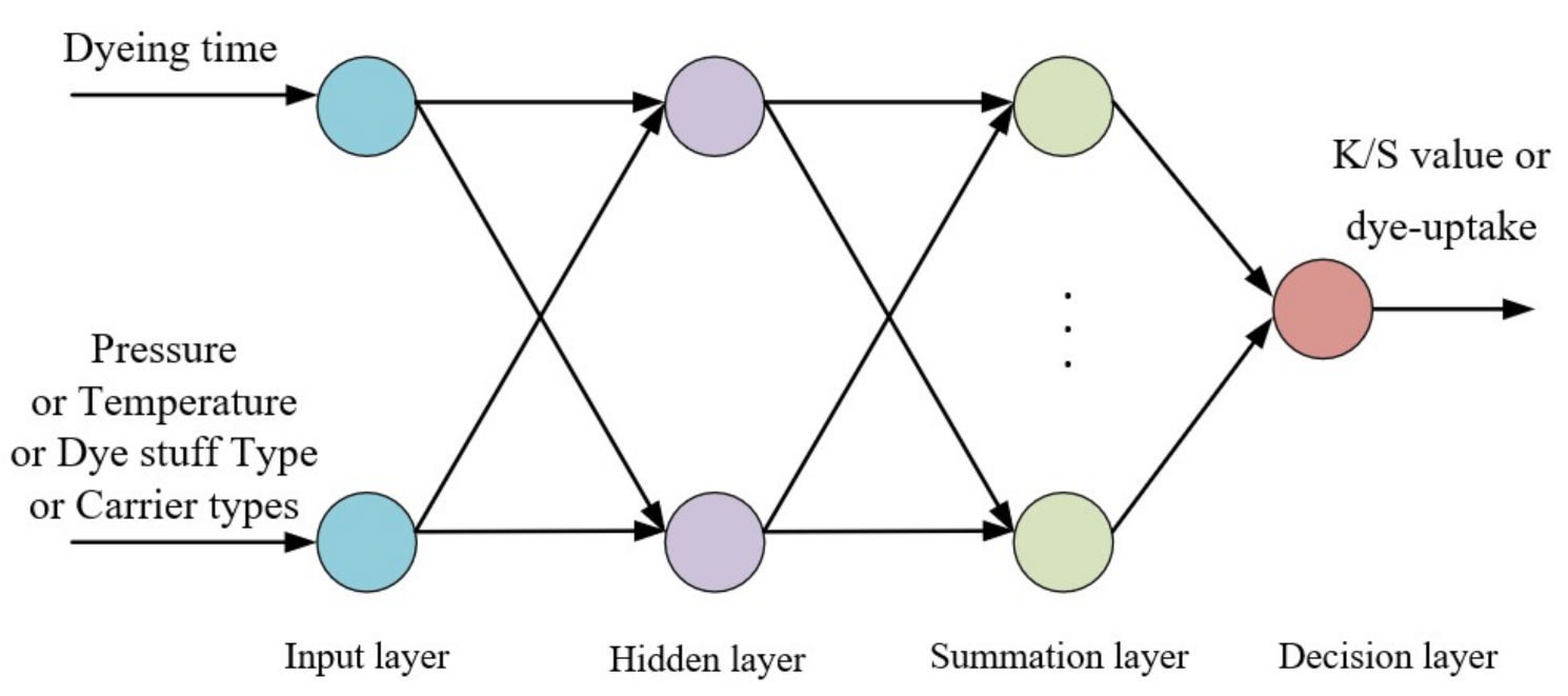
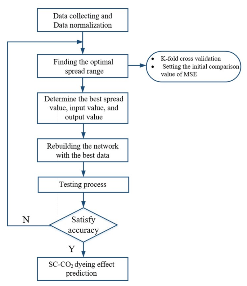
2.2. GRNN Description
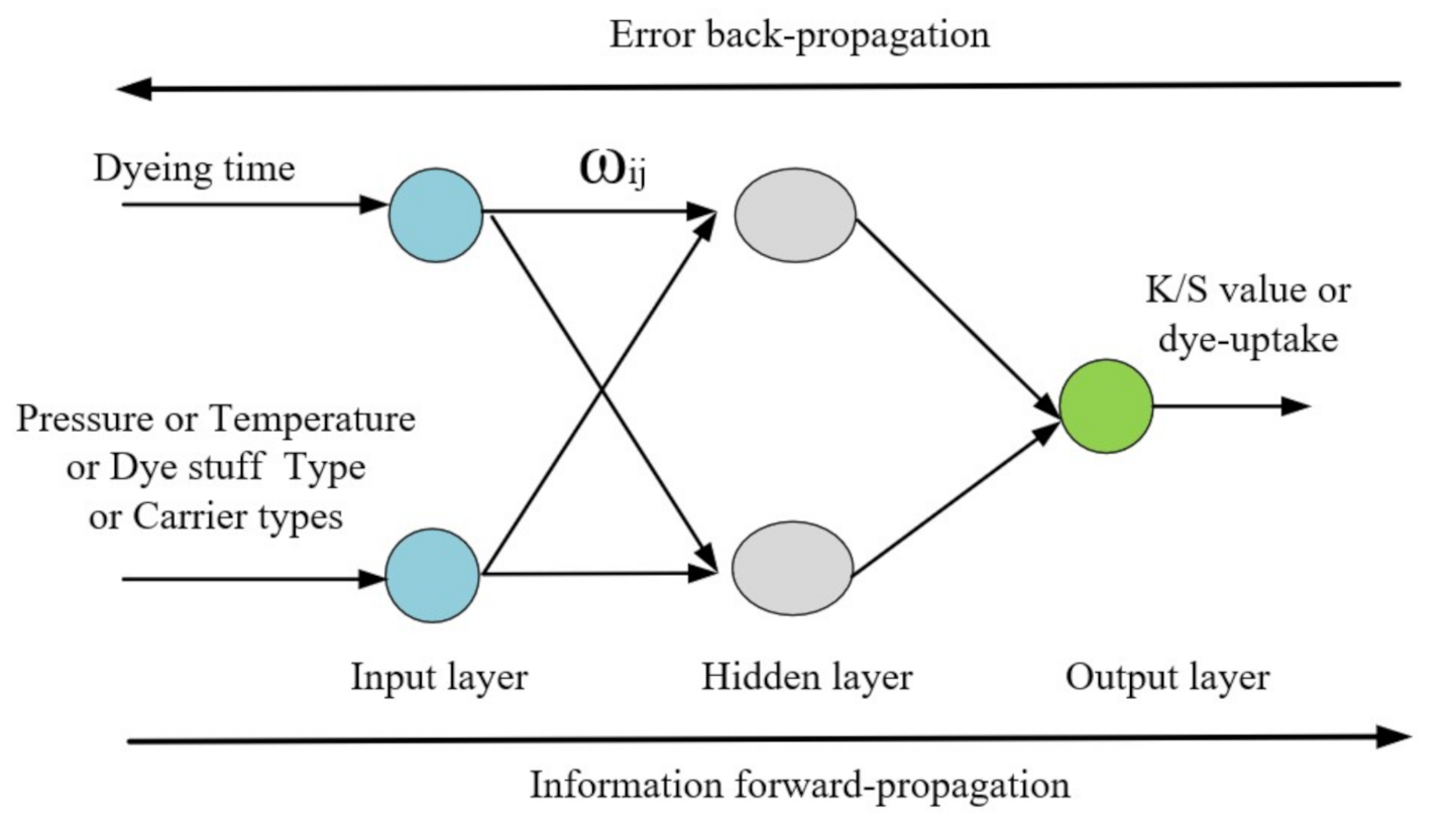
2.3. BPNN Description
2.4. Performance Criteria
3. Results and Discussion
3.1. The SC-CO2 Dyeing Effect Prediction Using GRNN
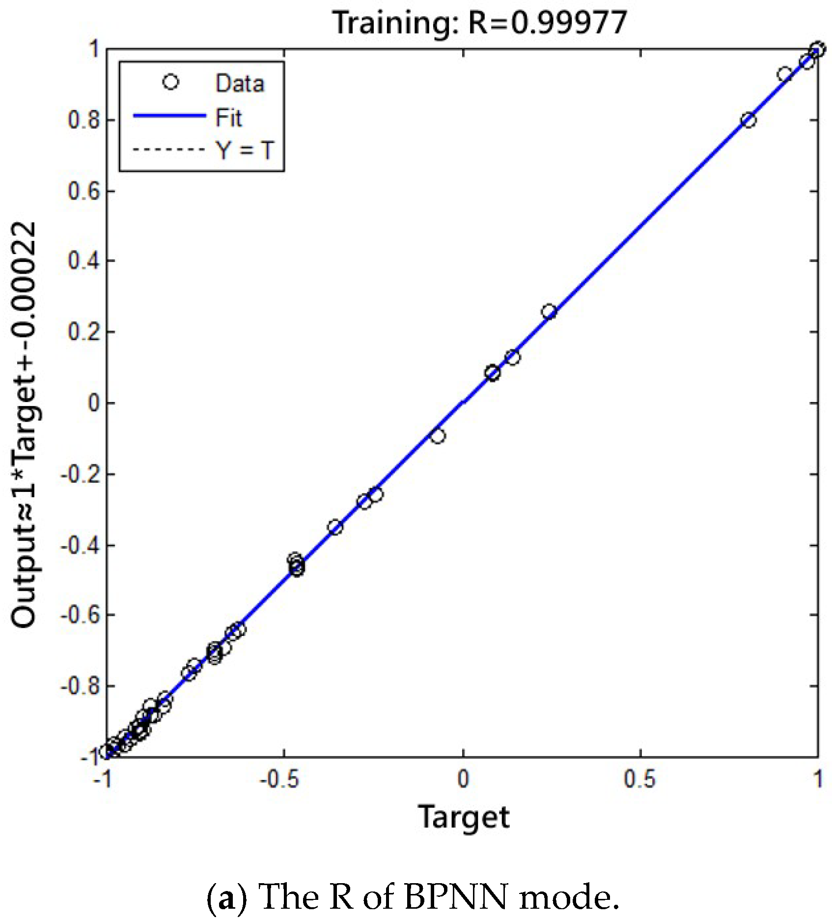
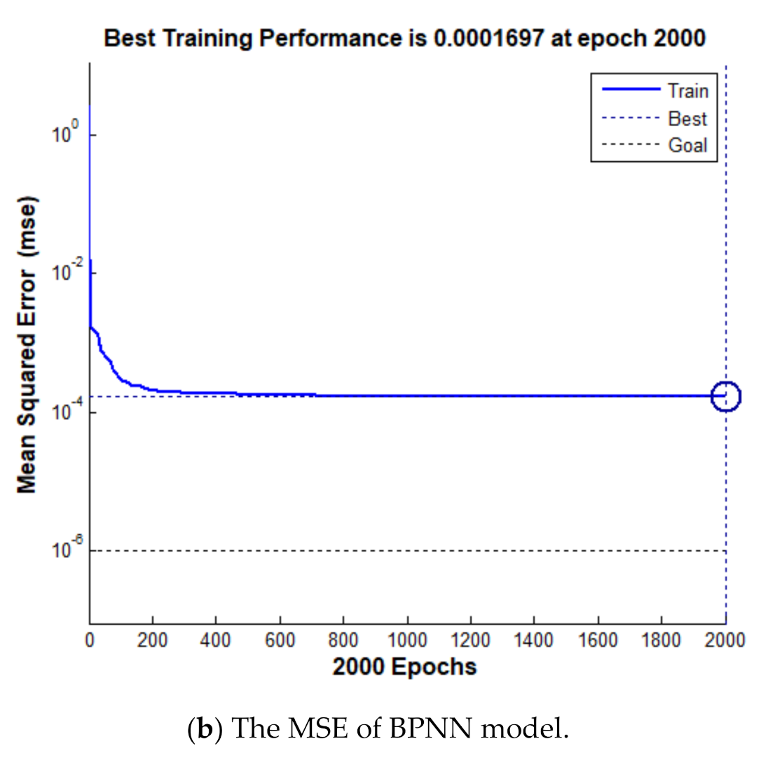
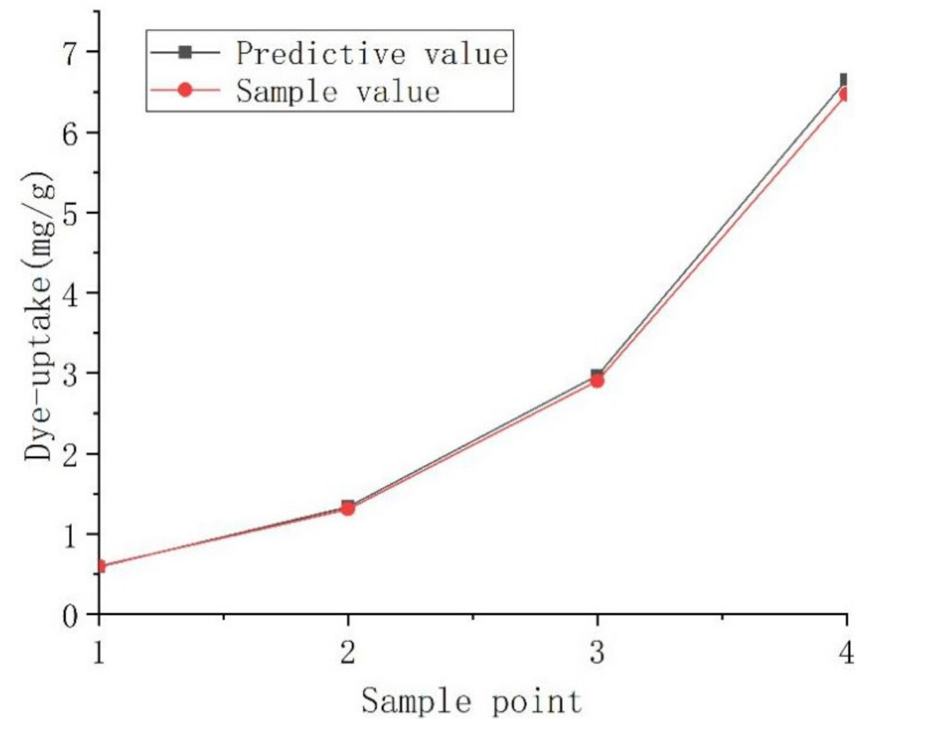
3.2. The SC-CO2 Dyeing Effect Prediction Using BPNN
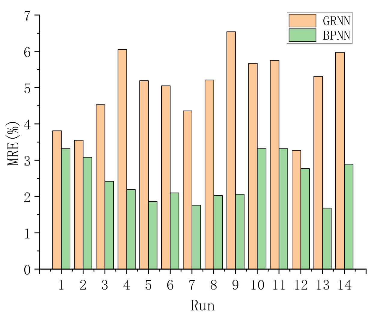
3.3. Comparing GRNN And BPNN Modelling
4. Conclusions
Supplementary Materials
Author Contributions
Funding
Acknowledgments
Conflicts of Interest
References
- Bai, T. Supercritical CO2 dyeing for nylon, acrylic, polyester and casein buttons and their optimum dyeing conditions by design of experiments. J. CO2 Util. 2019, 33, 253–261. [Google Scholar] [CrossRef]
- Khatri, A.; White, M. Sustainable dyeing technologies. J. Sustain. Appar. 2015, 135–160. [Google Scholar] [CrossRef]
- Liu, M.; Zhao, H.J.; Wu, J.S.; Xiong, X.Q.; Zheng, L.J. Eco-friendly curcumin-based dyes for supercritical carbon dioxide natural fabric dyeing. J. Clean. Prod. 2018, 197, 1262–1267. [Google Scholar] [CrossRef]
- Kim, T.; Seo, B.; Park, G.; Lee, Y.W. Effects of dye particle size and dissolution rate on the overall dye uptake in supercritical dyeing process. J. Supercrit. Fluids 2019, 151, 1–7. [Google Scholar] [CrossRef]
- Elmaaty, T.A.; El-Taweel, F.; Elsisi, H.; Okubayashi, S. Water free dyeing of polypropylene fabric under supercritical carbon dioxide and comparison with its aqueous analogue. J. Supercrit. Fluids 2018, 139, 114–121. [Google Scholar] [CrossRef]
- Sicardi, S.; Manna, L.; Banchero, M. Comparison of dye diffusion in poly(ethylene terephthalate) films in the presence of a supercritical or aqueous solvent. Ind. Eng. Chem. Res. 2000, 39, 4707–4713. [Google Scholar] [CrossRef]
- Sicardi, S.; Manna, L.; Banchero, M. Diffusion of disperse dyes in PET films during impregnation with a supercritical fluid. J. Supercrit. Fluids 2000, 17, 187–194. [Google Scholar] [CrossRef]
- Casetta, M.; Koncar, V.; Cazé, C. Mathematical modeling of the diffusion coeffificient for disperse dyes. Text. Res. J. 2001, 71, 357–361. [Google Scholar] [CrossRef]
- Banchero, M.; Ferri, A. Simulation of aqueous and supercritical fluid dyeing of a spool of yarn. J. Supercrit. Fluids 2005, 35, 157–166. [Google Scholar] [CrossRef]
- Fleming, O.S.; Stepanek, F.; Kazarian, S.G. Dye diffusion in polymer films subjected to supercritical CO2: Confocal raman microscopy and modelling. Macromol. Chem. Phys. 2005, 206, 1077–1083. [Google Scholar] [CrossRef]
- Özcan, A.S.; Özcan, A. Adsorption behavior of a disperse dye on polyester in supercritical carbon dioxide. J. Supercrit. Fluids 2005, 35, 133–139. [Google Scholar] [CrossRef]
- Tu, J.; Wei, X.H.; Huang, B.B.; Fan, H.B.; Jian, M.F.; Li, W. Improvement of sap flow estimation by including phenological index and time-lag effect in back-propagation neural network models. Agric. Forest Meteorol. 2019, 276, 107608. [Google Scholar] [CrossRef]
- Castano, F.; Beruvides, G.; Haber, R.E.; Artuñedo, A. Obstacle recognition based on machine learning for on-chip LiDAR sensors in a cyber-physical system. Sensors 2017, 17, 2109. [Google Scholar] [CrossRef] [PubMed] [Green Version]
- Ni, Y.Q.; Li, M. Wind pressure data reconstruction using neural network techniques: A comparison between BPNN and GRNN. Measurement 2016, 88, 468–476. [Google Scholar] [CrossRef]
- Chen, Y.; Shen, L.; Li, R.; Xu, X.; Hong, H.; Lin, H.; Chen, J. Quantification of interfacial energies associated with membrane fouling in a membrane bioreactor by using BP and GRNN artificial neural networks. J. Colloid Interface Sci. 2020, 565, 1–10. [Google Scholar] [CrossRef]
- Sun, W.; Gao, Q. Exploration of energy saving potential in China power industry based on Adaboost back propagation neural network. J. Clean. Prod. 2019, 217, 257–266. [Google Scholar] [CrossRef]
- Ye, Z.Y.; Kim, M.K. Predicting electricity consumption in a building using an optimized back-propagation and Levenberg–Marquardt back-propagation neural network: Case study of a shopping mall in China. Sustain. Cities Soc. 2018, 42, 176–183. [Google Scholar] [CrossRef]
- Fernández-Gámez, M.A.; Gil-Corral, A.M.; Galán-Valdivieso, F. Corporate reputation and market value: Evidence with generalized regression neural networks. Expert Syst. Appl. 2016, 46, 69–76. [Google Scholar] [CrossRef]
- Kumar, G.; Malik, H. Generalized regression neural network based wind speed prediction model for Western Region of India. Procedia Comput. Sci. 2016, 93, 26–32. [Google Scholar] [CrossRef] [Green Version]
- Bendu, H.; Deepak, B.; Murugan, S. Application of GRNN for the prediction of performance and exhaust emissions in HCCI engine using ethanol. Energy Convers. Manag. 2016, 122, 165–173. [Google Scholar] [CrossRef]
- Khajeh, M.; Moghaddam, M.G.; Shakeri, M. Application of artificial neural network in predicting the extraction yield of essential oils of Diplotaenia cachrydifolia by supercritical fluid extraction. J. Supercrit. Fluids 2012, 69, 91–96. [Google Scholar] [CrossRef]
- Bhupendra, S.; Bikash, M. Application of an artificial neural network model for the supercritical fluid extraction of seed oil from, Argemone mexicana, (L.) seeds. Ind. Crop. Prod. 2018, 123, 64–74. [Google Scholar]
- Kuvendziev, S.; Lisichkov, K.; Zeković, Z.; Marinkovski, M. Artificial neural network modelling of supercritical fluid CO2 extraction of polyunsaturated fatty acids from common carp (Cyprinus carpio L.) viscera. J. Supercrit. Fluids 2014, 92, 242–248. [Google Scholar] [CrossRef]
- Izadifar, M.; Abdolahi, F. Comparison between neural network and mathematical modeling of supercritical CO2 extraction of black pepper essential oil. J. Supercrit. Fluids 2006, 38, 37–43. [Google Scholar] [CrossRef]
- Aminian, A. Estimating the solubility of different solutes in supercritical CO2 covering a wide range of operating conditions by using neural network models. J. Supercrit. Fluids 2017, 125, 79–87. [Google Scholar] [CrossRef]
- Khazaiepoul, A.; Soleimani, M.; Salahi, S. Solubility prediction of disperse dyes in supercritical carbon dioxide and ethanol as co-solvent using neural network. Chin. J. Chem. Eng. 2016, 24, 491–498. [Google Scholar] [CrossRef]
- Bakhbakhi, Y. Phase equilibria prediction of solid solute in supercritical carbon dioxide with and without a cosolvent: The use of artificial neural network. Expert Syst. Appl. 2011, 38, 11355–11362. [Google Scholar] [CrossRef]
- Ye, K.; Zhang, Y.; Yang, L.; Zhao, Y.; Li, N.; Xie, C. Modeling convective heat transfer of supercritical carbon dioxide using an artificial neural network. Appl. Therm. Eng. 2019, 150, 686–695. [Google Scholar] [CrossRef]
- Hou, A.Q.; Chen, B.; Dai, J.J.; Zhang, K. Using supercritical carbon dioxide as solvent to replace water in polyethylene terephthalate (PET) fabric dyeing procedures. J. Clean. Prod. 2010, 18, 1009–1014. [Google Scholar] [CrossRef]
- Liu, Z.T.; Zhang, L.L.; Liu, Z.W.; Gao, Z.; Dong, W.S.; Xiong, H.P.; Peng, Y.; Tang, S.W. Supercritical CO2 Dyeing of Ramie Fiber with Disperse Dye. Ind. Eng. Chem. Res. 2006, 45, 8932–8938. [Google Scholar] [CrossRef]
- Zheng, H.D.; Zheng, L.J. Dyeing of Meta-aramid Fibers with Disperse Dyes in Supercritical Carbon Dioxide. Fiber. Polym. 2014, 15, 1627–1634. [Google Scholar] [CrossRef]
- Zhang, H.Z.; Zhong, Z.L.; Feng, L.L.; Quan, X.P. Research on Polypropylene Dyeing in Supercritical Carbon Dioxide. Adv. Mater. Res. 2011, 175–176, 646–650. [Google Scholar] [CrossRef]
- Zheng, H.D.; Zhang, J.; Yan, J.; Zheng, L.J. Investigations on the effect of carriers on meta-aramid fabric dyeing properties in supercritical carbon dioxide. Rsc. Adv. 2017, 7, 3470–3479. [Google Scholar] [CrossRef] [Green Version]
- Hou, A.; Dai, J. Kinetics of dyeing of polyester with CI Disperse Blue 79 in supercritical carbon dioxide. Color. Technol. 2010, 121, 18–20. [Google Scholar] [CrossRef]
- Chang, H.K.; Bae, H.K.; Shim, J.J. Dyeing of pet textile fibers and films in supercritical carbon dioxide. Korean J. Chem. Eng. 1996, 13, 310–316. [Google Scholar] [CrossRef]
- Ömer, K. An efficient and robust deep learning based network anomaly detection against distributed denial of service attacks. Comput. Netw. 2020, 180, 107390. [Google Scholar]
- Sodeifian, G.; Sajadian, S.A.; Ardestani, N.S. Evaluation of the response surface and hybrid artificial neural network-genetic algorithm methodologies to determine extraction yield of Ferulago angulata through supercritical fluid. J. Taiwan Inst. Chem. Eng. 2016, 60, 165–173. [Google Scholar] [CrossRef]
- Ayegba, P.O.; Abdulkadir, M.; Hernandez-Perez, V.; Lowndes, I.S.; Azzopardi, B.J. Applications of artificial neural network (ANN) method for performance prediction of the effect of a vertical 90° bend on an air–silicone oil flow. J. Taiwan Inst. Chem. Eng. 2017, 74, 59–64. [Google Scholar] [CrossRef]
- Ameer, K.; Chun, B.S.; Kwon, J.H. Optimization of supercritical fluid extraction of steviol glycosides and total phenolic content from Stevia rebaudiana (Bertoni) leaves using response surface methodology and artificial neural network modeling. Ind. Crop. Prod. 2017, 109, 672–685. [Google Scholar] [CrossRef]


| Group | Training Data Points | Testing and Prediction Data Points | Input Parameter | Output Parameter | References |
|---|---|---|---|---|---|
| 1 | 38 | 4 | Dyeing time, Temperature | K/S value | [29] |
| 2 | 32 | 4 | Pressure, Temperature | K/S value | [30] |
| 3 | 21 | 3 | Dyeing time, Temperature | K/S value | [30] |
| 4 | 24 | 3 | Dye stuff types, Temperature | K/S value | [31] |
| 5 | 24 | 3 | Dye stuff types, Pressure | K/S value | [31] |
| 6 | 24 | 3 | Dye stuff types, Dyeing time | K/S value | [31] |
| 7 | 27 | 3 | Pressure, Temperature | K/S value | [32] |
| 8 | 22 | 3 | Pressure, Dyeing time | K/S value | [32] |
| 9 | 17 | 3 | Carrier types, Temperature | K/S value | [33] |
| 10 | 17 | 3 | Carrier types, Pressure | K/S value | [33] |
| 11 | 17 | 3 | Carrier types, Dyeing time | K/S value | [33] |
| 12 | 44 | 4 | Dyeing time, Temperature | Dye-uptake | [34] |
| 13 | 22 | 3 | Dyeing time, Pressure | Dye-uptake | [35] |
| 14 | 12 | 3 | Dyeing time, Temperature | Dye-uptake | [35] |
| Dyeing Time/min | Temperature/℃ | |||||
|---|---|---|---|---|---|---|
| 80 | 90 | 100 | 110 | 120 | 130 | |
| 5 | 0.2541 | 0.3462 | 0.8277 | 1.1755 | 2.2836 | 4.4031 |
| 10 | 0.3499 | 0.5418 | 1.0071 | 1.6659 | 3.2744 | 6.8232 |
| 15 | 0.4278 | 0.6011 * | 1.1423 | 2.1402 | 3.9331 | 7.3911 |
| 20 | 0.5381 | 0.7213 | 1.3102 * | 2.3565 | 4.5776 | 10.6401 |
| 30 | 0.6129 | 0.8382 | 1.5671 | 2.9022 * | 5.5899 | 11.2103 |
| 40 | 0.7611 | 0.9478 | 1.9735 | 3.3208 | 6.4723* | 11.5848 |
| 60 | 0.7631 | 0.9503 | 1.9856 | 3.3215 | 6.4823 | 11.7302 |
| 90 | 0.763 | 0.9506 | 1.9853 | 3.3217 | 6.4834 | 11.7401 |
| Run | Data Capacity | Best Spread Value | MSE | MRE (%) | Run | Data Capacity | Best Spread Value | MSE | MRE (%) |
|---|---|---|---|---|---|---|---|---|---|
| 1 | 42/4 | 0.18 | 0.1446 | 3.81 | 8 | 25/3 | 0.1 | 0.0012 | 5.21 |
| 2 | 36/4 | 0.24 | 0.0916 | 3.55 | 9 | 20/3 | 0.32 | 0.0002 | 6.54 |
| 3 | 24/3 | 0.34 | 0.0449 | 4.53 | 10 | 20/3 | 0.32 | 0.0056 | 5.67 |
| 4 | 27/3 | 0.22 | 0.0061 | 6.05 | 11 | 20/3 | 0.28 | 0.0037 | 5.75 |
| 5 | 27/3 | 0.34 | 0.0001 | 5.19 | 12 | 48/4 | 0.24 | 0.0183 | 3.27 |
| 6 | 27/3 | 0.26 | 0.0022 | 5.05 | 13 | 25/3 | 0.54 | 2.4014 | 5.31 |
| 7 | 30/3 | 0.26 | 0.0001 | 4.36 | 14 | 15/3 | 0.32 | 0.0001 | 5.97 |
| Training Function | MSE | R | MRE |
|---|---|---|---|
| Traingdx | 1.2392*10−5 | 0.99852 | 0.29 |
| L-M | 9.4492*10−6 | 0.99981 | 0.1446 |
| Run | Data Capacity | Network Structure | R | MSE | MRE (%) | Run | Data Capacity | Network Structure | R | MSE | MRE (%) |
|---|---|---|---|---|---|---|---|---|---|---|---|
| 1 | 42/4 | 2/7/1 | 0.99981 | 9.4492 × 10⁻⁶ | 3.32 | 8 | 25/3 | 2/7/1 | 0.99954 | 1.70 × 10⁻⁵ | 2.03 |
| 2 | 36/4 | 2/7/1 | 0.99971 | 6.64 × 10⁻⁵ | 3.08 | 9 | 20/3 | 2/7/1 | 0.99932 | 4.95E × 10−7 | 2.06 |
| 3 | 24/3 | 2/7/1 | 0.99983 | 2.79 × 10⁻¹² | 2.42 | 10 | 20/3 | 2/7/1 | 0.99941 | 4.01 × 10⁻⁷ | 3.33 |
| 4 | 27/3 | 2/7/1 | 0.99991 | 9.54 × 10⁻⁷ | 2.19 | 11 | 20/3 | 2/7/1 | 0.99901 | 4.90 × 10⁻⁷ | 3.30 |
| 5 | 27/3 | 2/7/1 | 0.99926 | 9.97 × 10⁻⁷ | 1.86 | 12 | 48/4 | 2/7/1 | 0.99911 | 6.431 × 10⁻⁴ | 2.77 |
| 6 | 27/3 | 2/7/1 | 0.99974 | 7.36 × 10⁷ | 2.1 | 13 | 25/3 | 2/7/1 | 0.99956 | 2.70 × 10⁻⁷ | 1.68 |
| 7 | 30/3 | 2/7/1 | 0.99988 | 1.33 × 10⁻⁵ | 1.76 | 14 | 15/3 | 2/7/1 | 0.99938 | 7.89 × 10⁻⁷ | 2.89 |
Publisher’s Note: MDPI stays neutral with regard to jurisdictional claims in published maps and institutional affiliations. |
© 2020 by the authors. Licensee MDPI, Basel, Switzerland. This article is an open access article distributed under the terms and conditions of the Creative Commons Attribution (CC BY) license (http://creativecommons.org/licenses/by/4.0/).
Share and Cite
Zhang, Z.; Sun, F.; Li, Q.; Wang, W.; Hu, D.; Li, S. Establishment of the Predicting Models of the Dyeing Effect in Supercritical Carbon Dioxide Based on the Generalized Regression Neural Network and Back Propagation Neural Network. Processes 2020, 8, 1631. https://doi.org/10.3390/pr8121631
Zhang Z, Sun F, Li Q, Wang W, Hu D, Li S. Establishment of the Predicting Models of the Dyeing Effect in Supercritical Carbon Dioxide Based on the Generalized Regression Neural Network and Back Propagation Neural Network. Processes. 2020; 8(12):1631. https://doi.org/10.3390/pr8121631
Chicago/Turabian StyleZhang, Zhuo, Fayu Sun, Qingling Li, Weiqiang Wang, Dedong Hu, and Shuangchun Li. 2020. "Establishment of the Predicting Models of the Dyeing Effect in Supercritical Carbon Dioxide Based on the Generalized Regression Neural Network and Back Propagation Neural Network" Processes 8, no. 12: 1631. https://doi.org/10.3390/pr8121631