Cryogenic Energy for Indirect Freeze Desalination—Numerical and Experimental Investigation

Abstract
:1. Introduction
2. CFD Modelling Theory
2.1. Evaporation of Liquid Nitrogen Theory
2.2. Freeze Desalination Process Theory
- , when T < Tsolidus
- , when T > Tliquidus
3. CFD Methodology
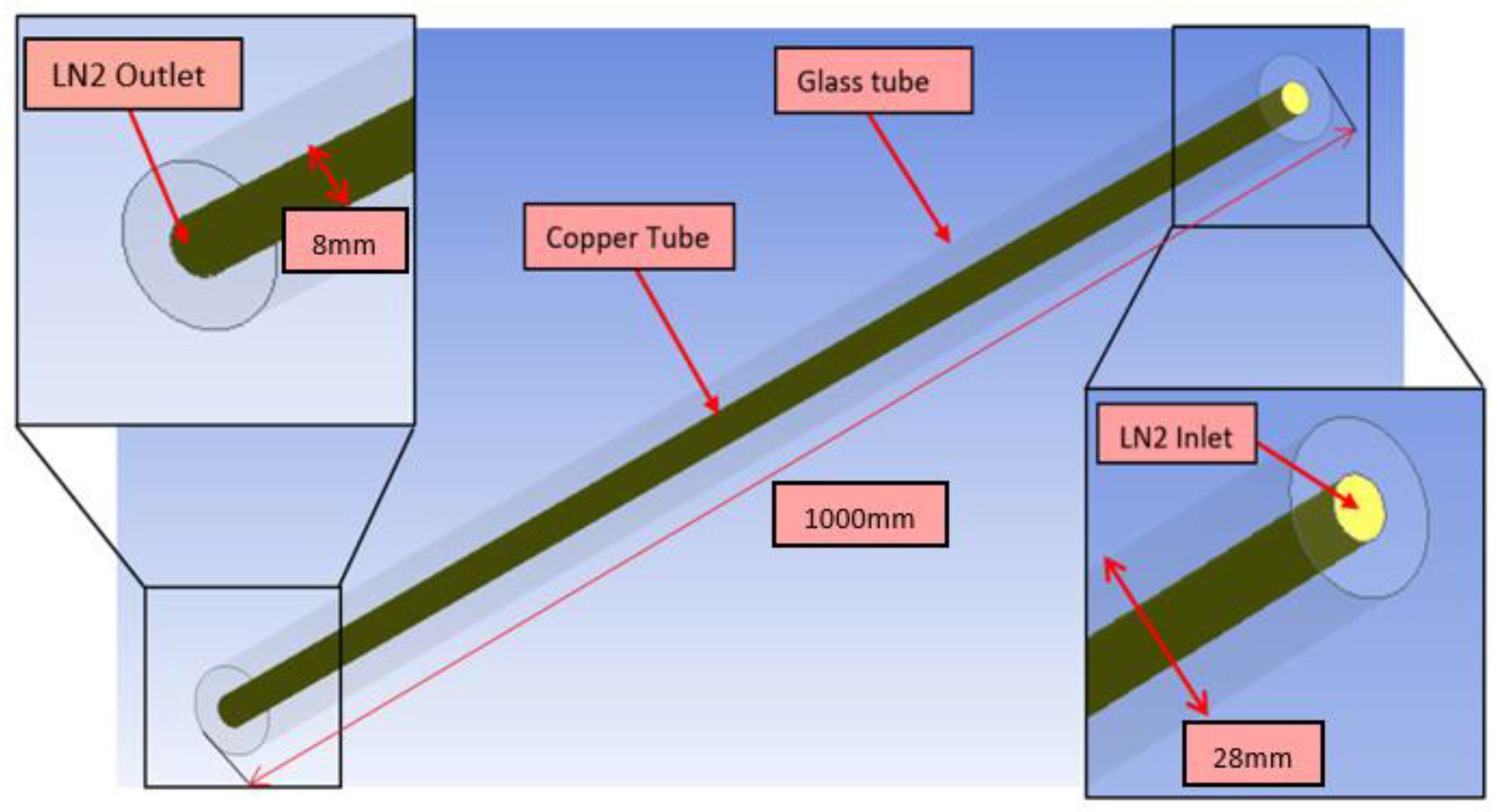
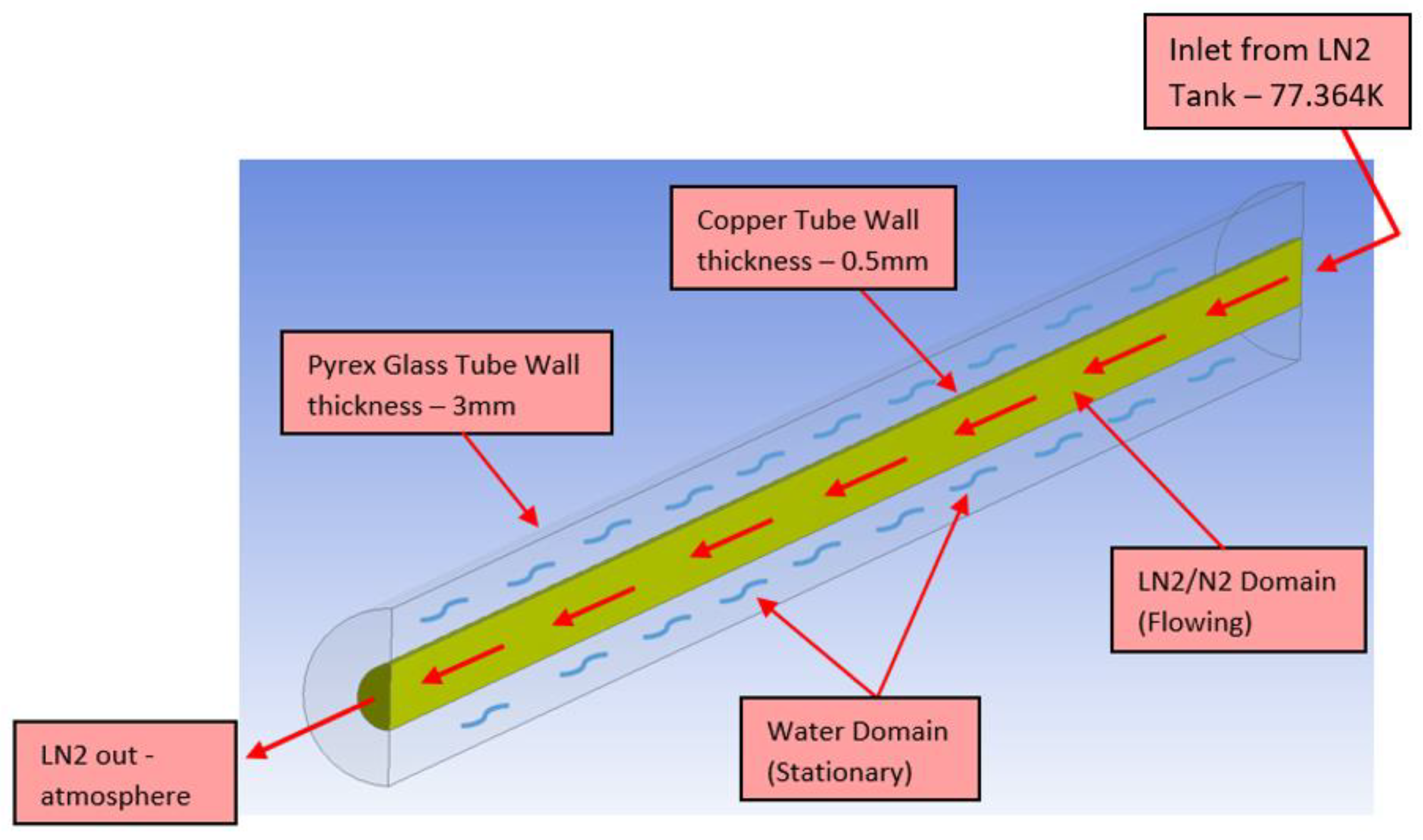
3.1. The Geometry
3.2. The Mesh
3.3. Set-Up
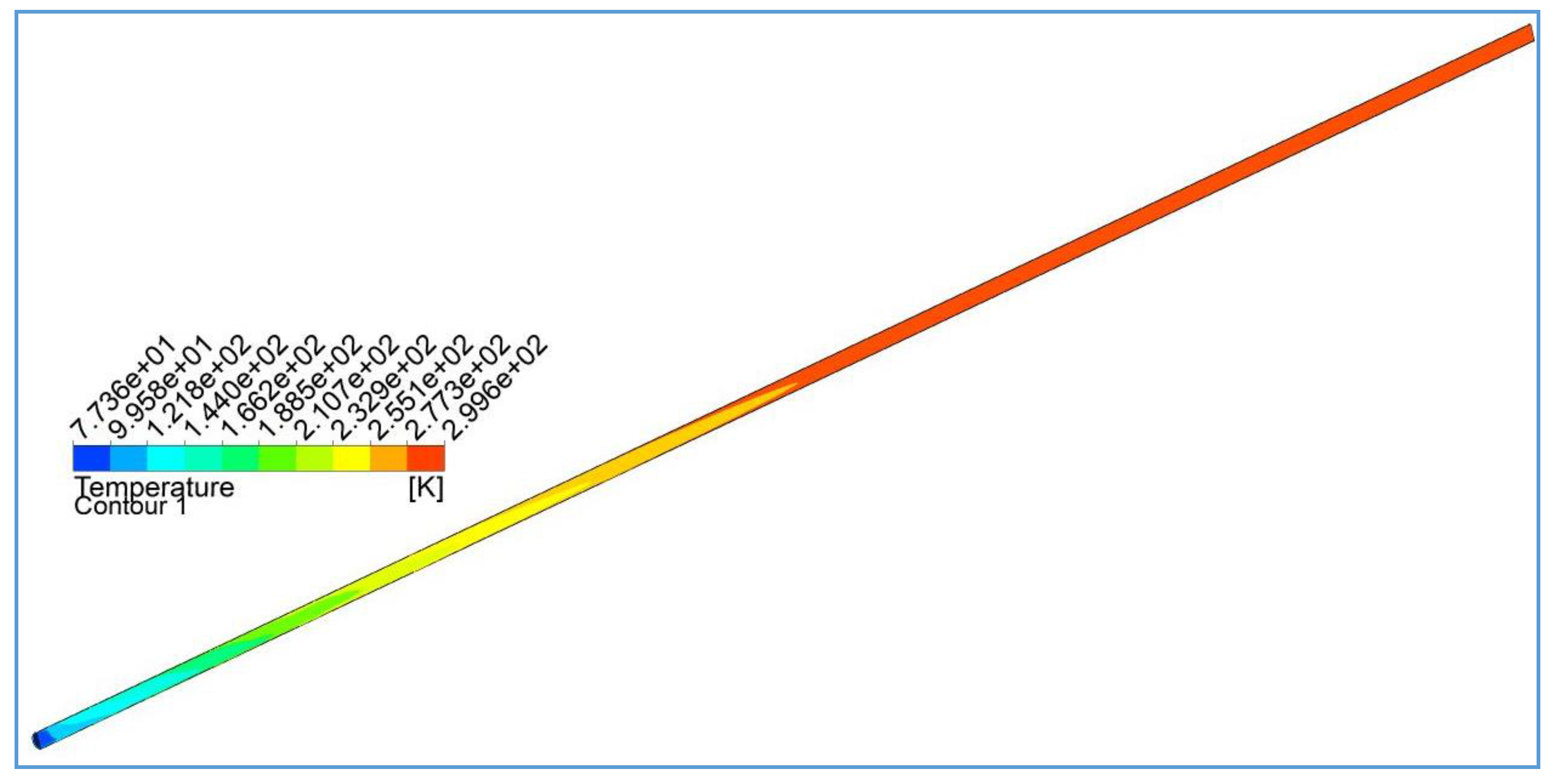
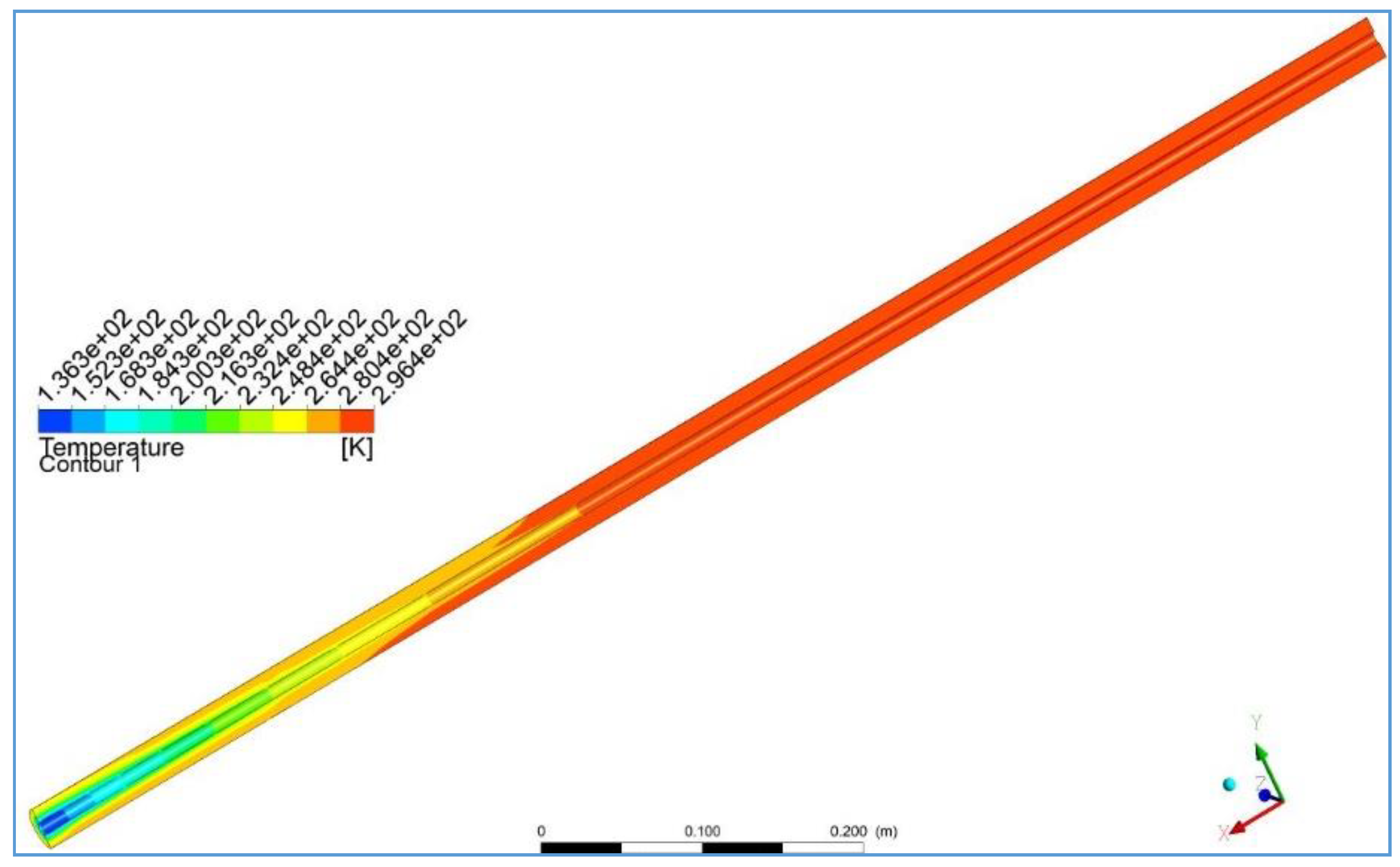
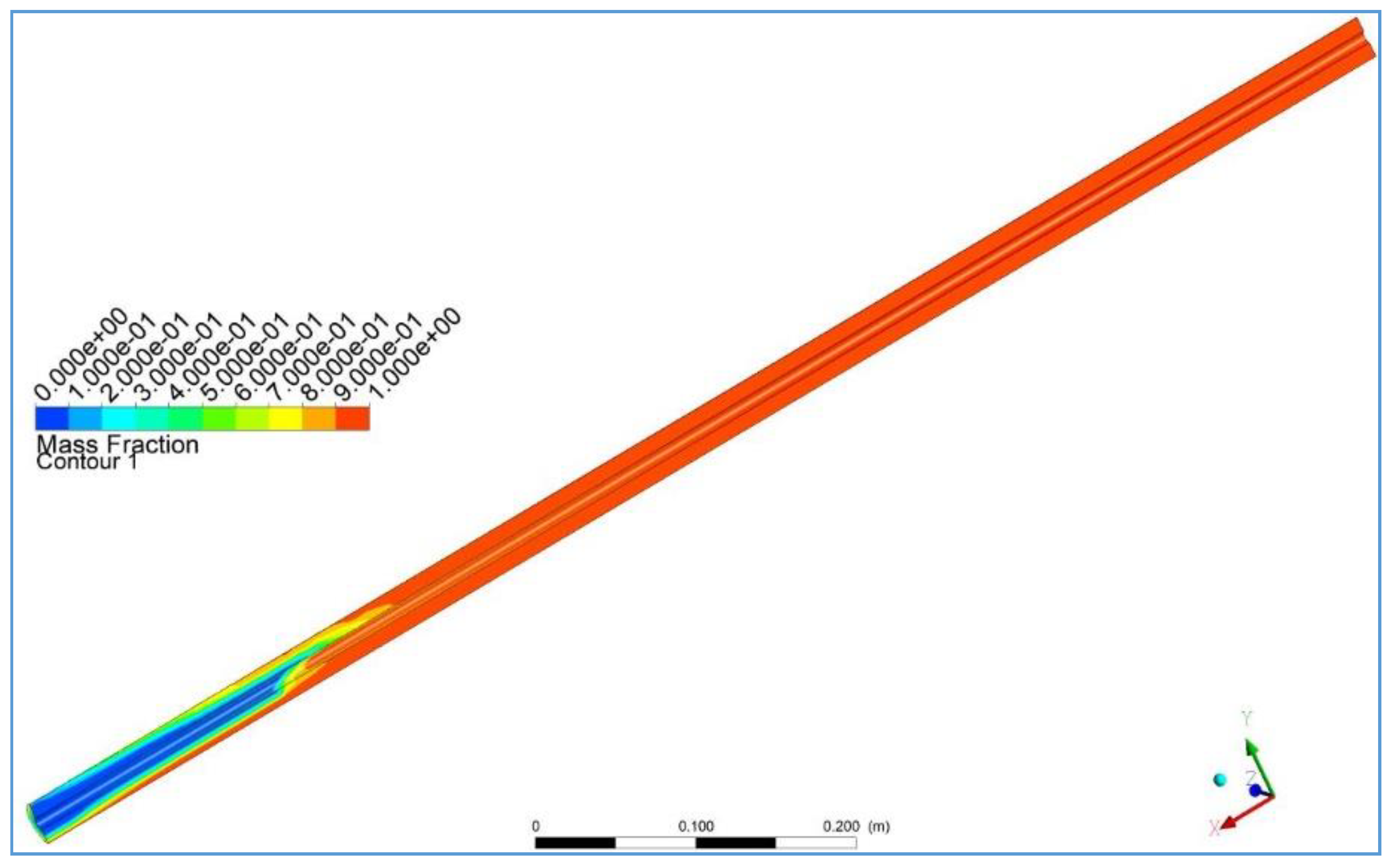
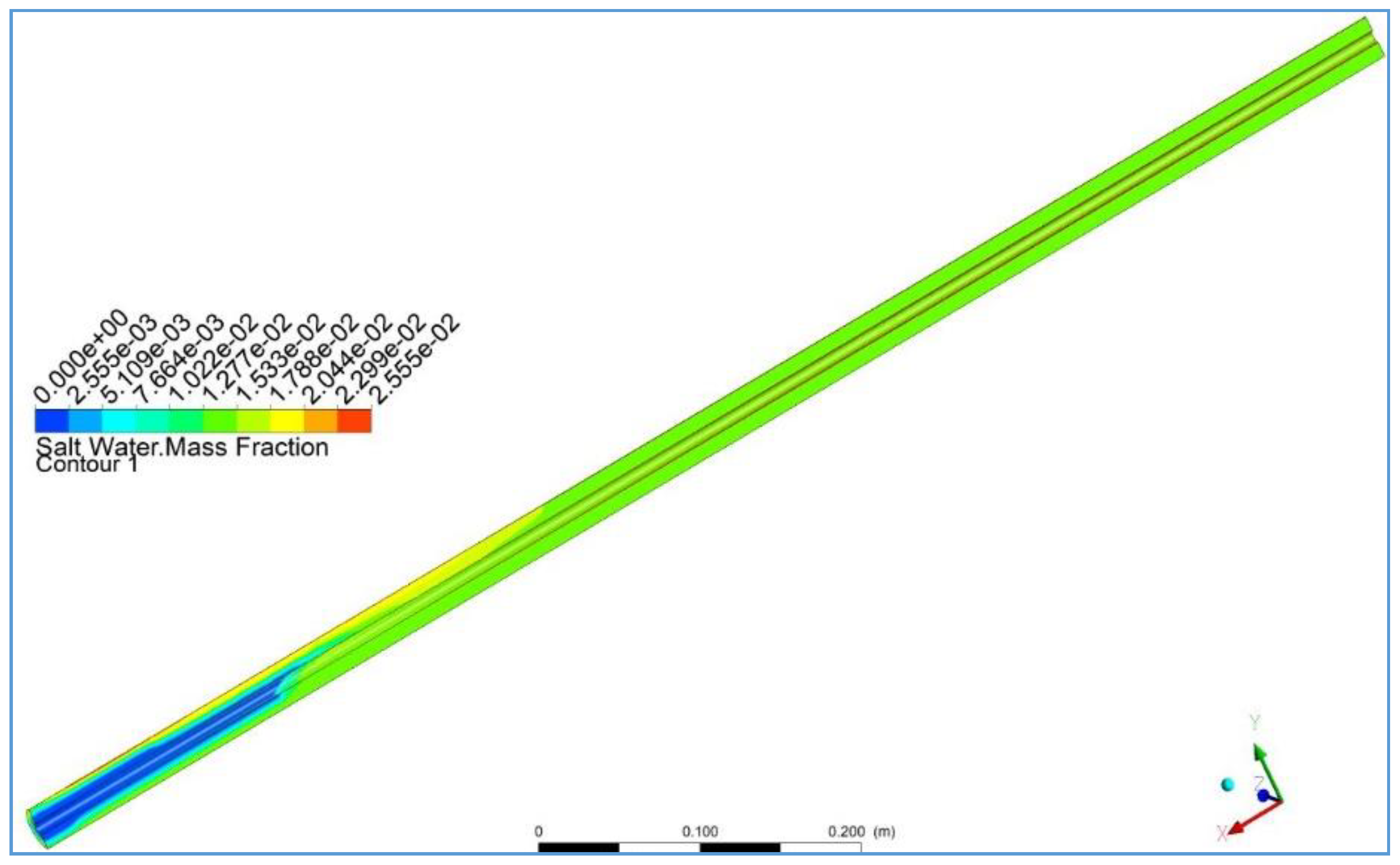
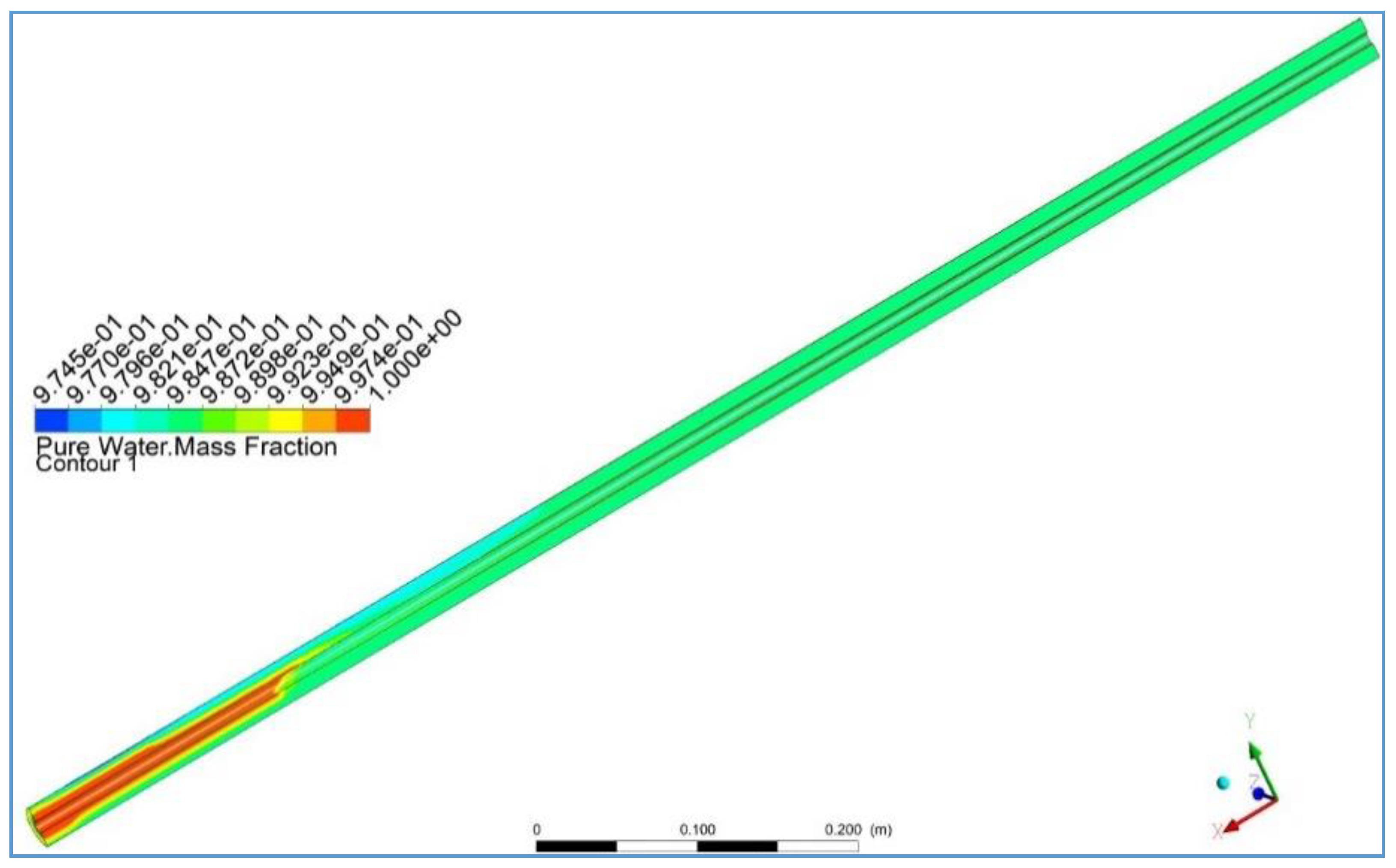
4. CFD Results
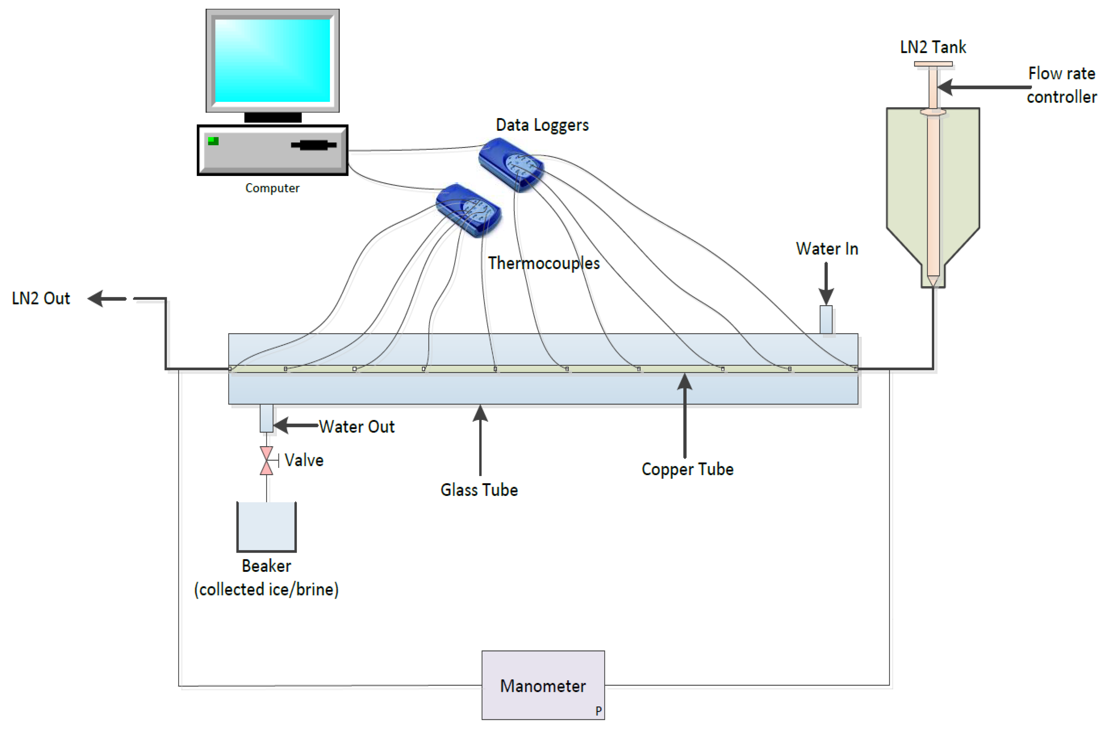
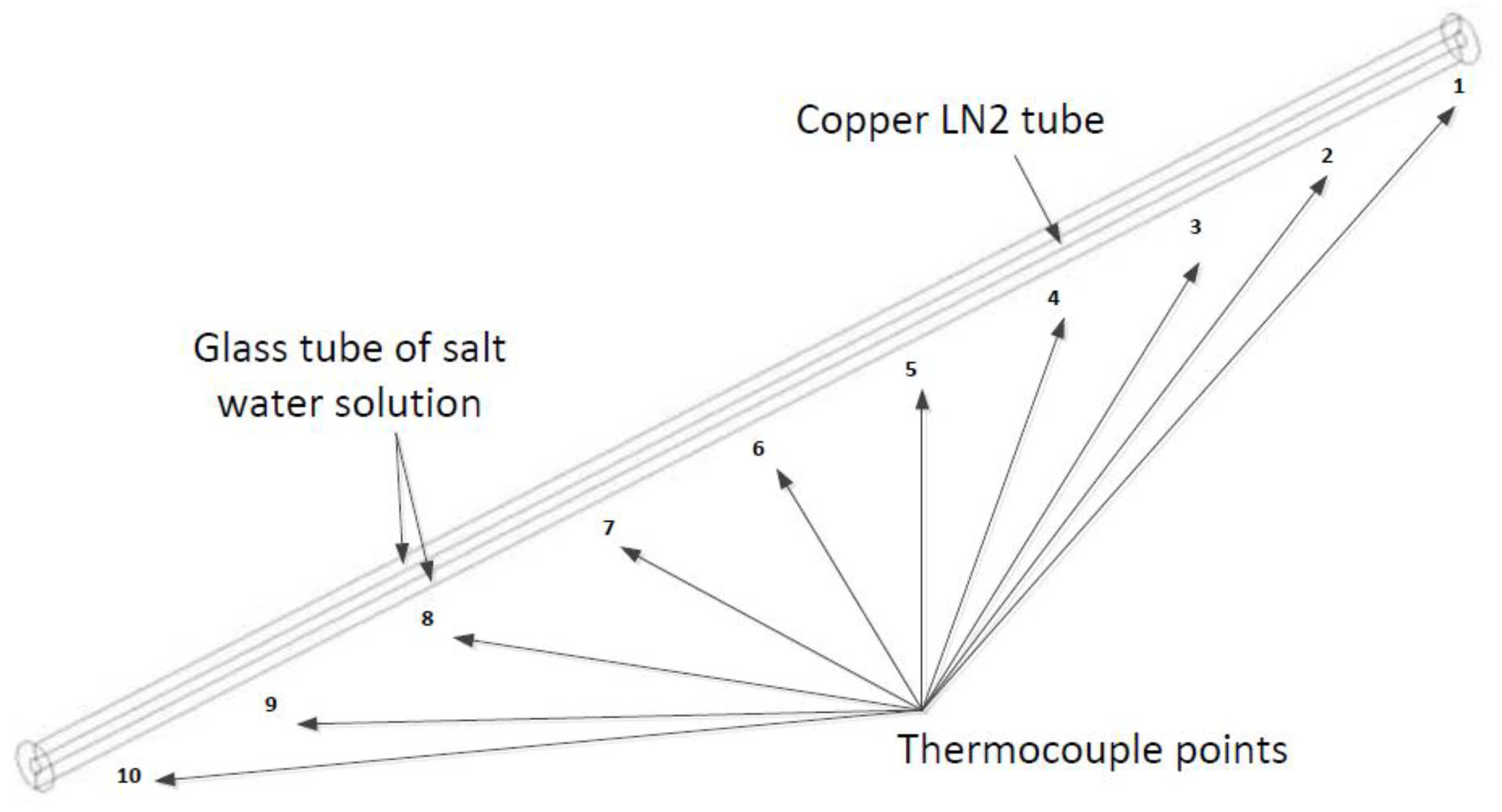
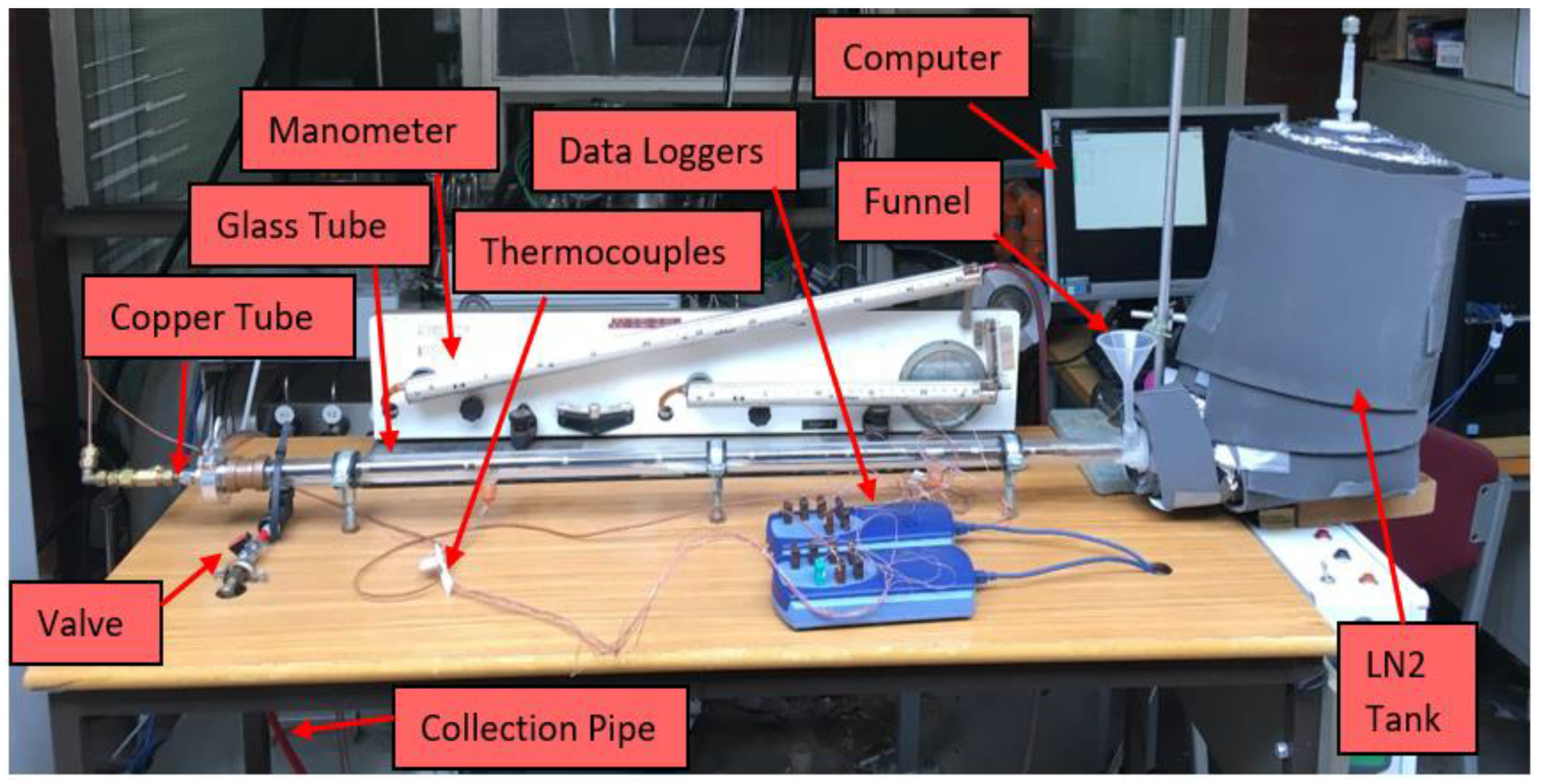
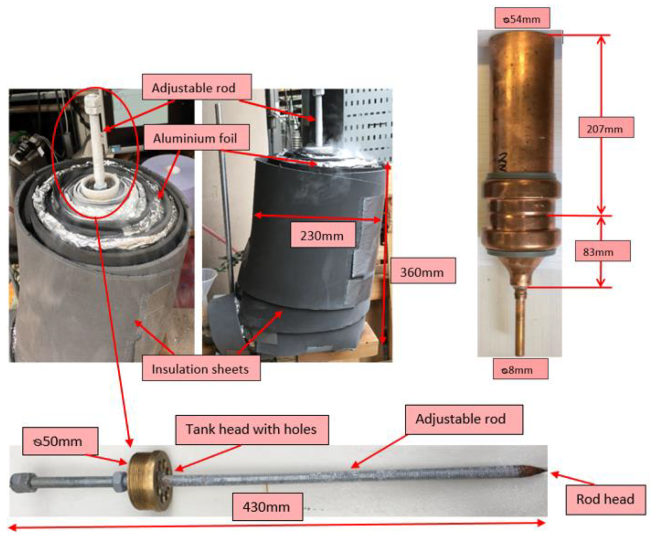
5. Experimental Test Facility
6. Experimental Results
6.1. Effect of Test Conditions on Temperature and Energy
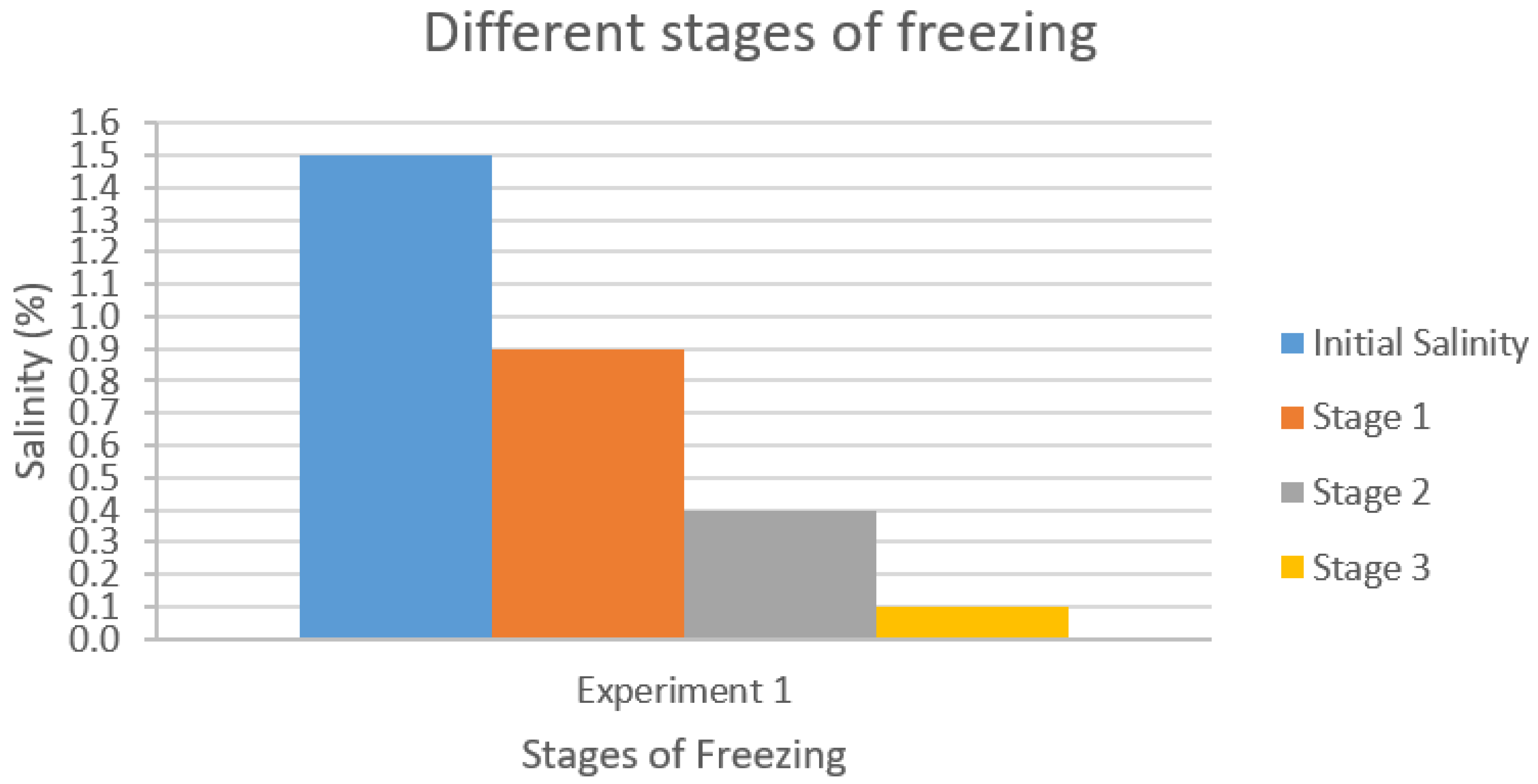
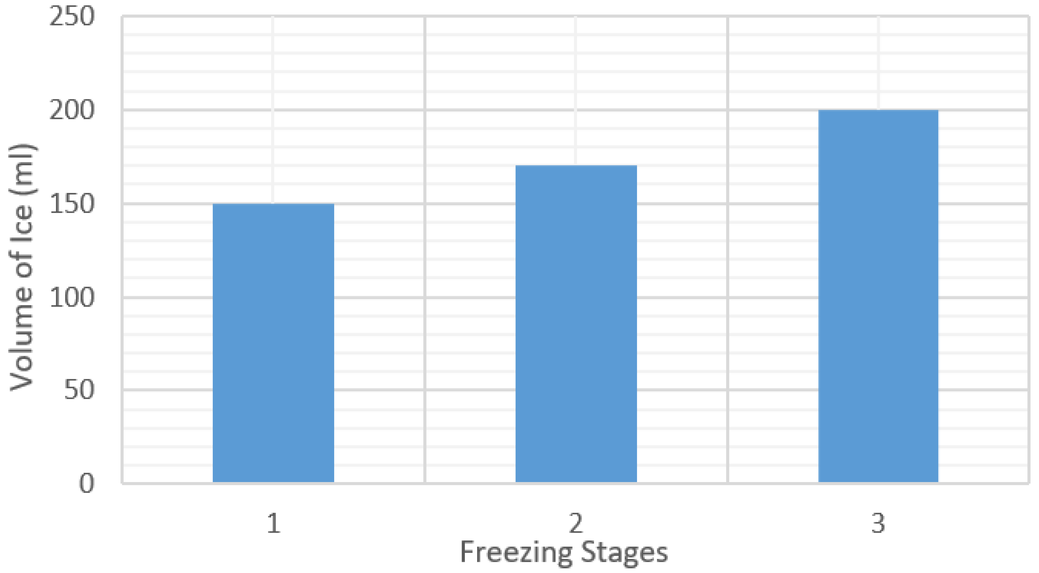
6.2. Effect of Test Conditions on Salinity and Volume of Ice
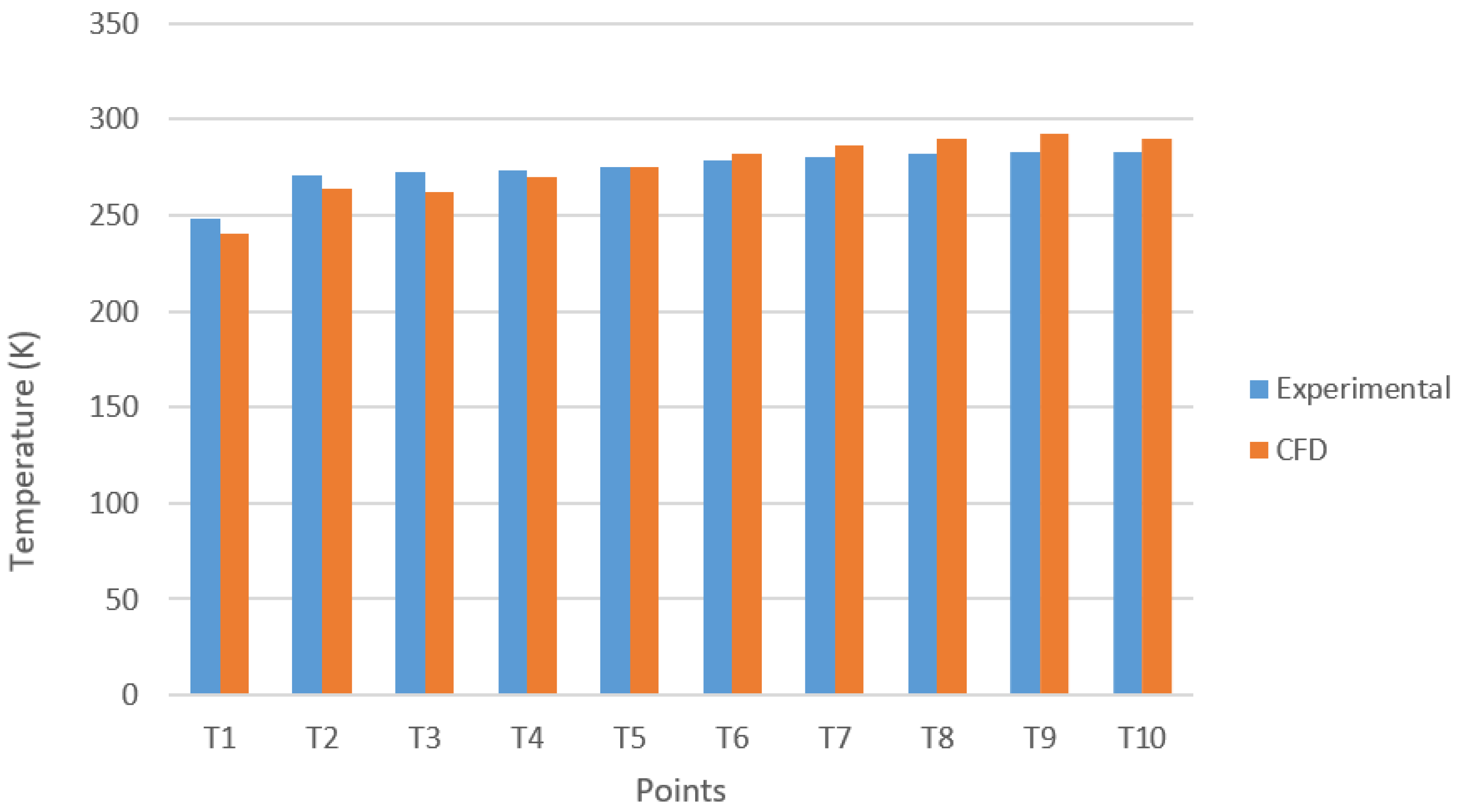
7. CFD Modelling Validation
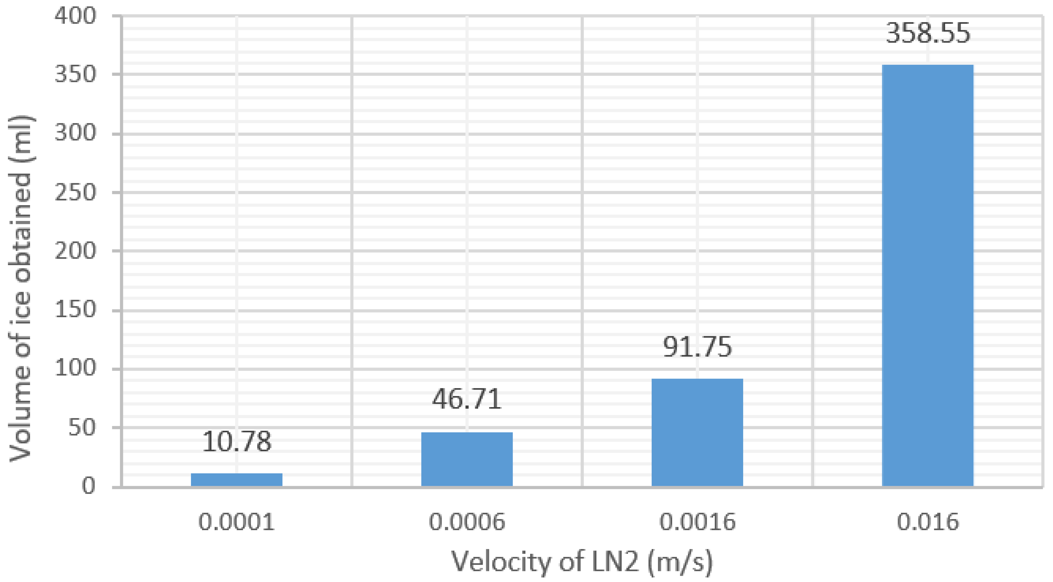
8. CFD Parametric Analysis—Flow Rate
9. Conclusions
Author Contributions
Funding
Acknowledgments
Conflicts of Interest
Nomenclature
| Symbols | |
| surface area (m2) | |
| mushy zone constant (-) | |
| smaller heat capacity (J.kg/K.s) | |
| initial specific heat capacity (J/K) | |
| final specific heat capacity (J/K) | |
| mass diffusion coefficient for species (m2/s) | |
| total energy in a known volume of liquid nitrogen (J) | |
| body force (N) | |
| solutal buoyancy body forces (N) | |
| gravity (m/s2) | |
| enthalpy [energy/mass (J/kg), energy/mole (J/mol)] | |
| inlet enthalpy (J/kg) | |
| outlet enthalpy (J/kg) | |
| diffusion flux of the species (kg/m2-s) | |
| effective conductivity (W/m-K) | |
| partition coefficient of the solute (-) | |
| latent heat (J/kg) | |
| latent heat of fusion (J/kg) | |
| mass (kg) | |
| mass flow rate (kg/s) | |
| rate of mass transfer from phase q to phase p (kg/s) | |
| rate of mass transfer from phase p to phase q (kg/s) | |
| slope of the liquidus surface (K) | |
| number of phases (-) | |
| number of species (-) | |
| p | pressure (Pa) |
| energy lost by brine remaining (J) | |
| energy loss by ice (J) | |
| energy loss by water (J) | |
| source term | |
| influences from radiations and any other volumetric heat sources | |
| T | temperature (K) |
| inlet water temperature (K) | |
| outlet water temperature (K) | |
| inlet nitrogen temperature (K) | |
| inlet nitrogen temperature (K) | |
| U | overall heat transfer coefficient (W/m2K) |
| velocity (m/s) | |
| mass fraction of the solute (-) | |
| Greek Symbols | |
| volume fraction (-) | |
| liquid volume fraction (-) | |
| solutal expansion coefficient (K–1) | |
| small number (0.001) (-) | |
| effectiveness of the heat exchanger (-) | |
| viscosity of the fluid (Pa-s) | |
| density of fluid (kg/m3) | |
| Acronyms | |
| CFD | computational fluid dynamics |
| FD | freeze desalination |
| LNG | liquefied natural gas |
| LMTD | logarithmic mean temperature difference |
| NTU | number of transfer units |
| RO | reverse osmosis |
| F.P | freezing point |
| VOF | volume of fluid |
| Subscripts | |
| eutectic | |
| i | solute |
| liquid | |
| liquid | |
| liquid | |
| mixture | |
| melting | |
| N | nitrogen |
| secondary phase p | |
| qth phase | |
| reference | |
| s | species |
| saturated | |
| sol | solid |
| solid | |
| w | water |
| Superscripts | |
| ∗ | interface |
| temperature | |
References
- Mathioulakis, E.; Belessiotis, V.; Delyannis, E. Desalination by using alternative energy: Review and state-of-the-art. Desalination 2007, 203, 346–365. [Google Scholar] [CrossRef]
- Miller, J.E. Review of Water Resources and Desalination Techniques; Unlimited Release Report SAND-2003-0800; Sandia National Labs: Livermore, CA, USA, 2003. [Google Scholar]
- Engelman, J.W.R.; Cincotta, R.P.; Dye, B.; Gardner-Outlaw, T. People in the Balance: Population and Natural Resources at the Turn of the Millennium, Population; Population Action International: Washington, DC, USA, 2000. [Google Scholar]
- Clarke, M.B.T. Blue Gold: The Fight to Stop the Corporate Theft of the World’s Water. Contemp. Hum. Ecol. 2004, 11, 67–71. [Google Scholar]
- White, P.H.G.G.F. Water in Crisis: A Guide to the World’s Fresh Water Resources. Clim. Chang. 1993, 31, 119–122. [Google Scholar]
- March, H. The politics, geography, and economics of desalination: A critical review. Wiley Interdiscip. Rev. Water 2015, 2, 231–243. [Google Scholar] [CrossRef]
- Jayakody, H.; Al-Dadah, R.; Mahmoud, S. Numerical investigation of indirect freeze desalination using an ice maker machine. Energy Convers. Manag. 2018, 168, 407–420. [Google Scholar] [CrossRef]
- Burn, S.; Hoang, M.; Zarzo, D.; Olewniak, F.; Campos, E.; Bolto, B.; Barron, O. Desalinationtechniques-A review of the opportunities for desalination in agriculture. Desalination 2015, 364, 2–16. [Google Scholar] [CrossRef]
- Randall, D.G.J.N. A Succinct Review of the Treatment of Reverse Osmosis Brines Using Freeze Crystallization. J. Water Process Eng. 2015, 8, 186–194. [Google Scholar] [CrossRef]
- Fujioka, R.; Wang, L.P.; Dodbiba, G.; Fujita, T. Application of progressive freeze-concentration for desalination. Desalination 2013, 319, 33–37. [Google Scholar] [CrossRef]
- Attia, A.A.A. New proposed system for freeze water desalination using auto reversed R-22 vapor compression heat pump. Desalination 2010, 254, 179–184. [Google Scholar] [CrossRef]
- Williams, P.M.; Ahmad, M.; Connolly, B.S.; Oatley-Radcliffe, D.L. Technology for freeze concentration in the desalination industry. Desalination 2015, 356, 314–327. [Google Scholar] [CrossRef]
- Lu, Z.; Xu, L. Freezing Desalination Process. Desalin. Water Resour. 2014, 2, 275–290. [Google Scholar]
- Cao, W.; Beggs, C.; Mujtaba, I.M. Theoretical approach of freeze seawater desalination on flake ice maker utilizing LNG cold energy. Desalination 2014, 355, 22–32. [Google Scholar] [CrossRef] [Green Version]
- Curran, H.M. Water desalination by indirect freezing. Desalination 1970, 7, 273–284. [Google Scholar] [CrossRef]
- Lin, W.; Huang, M.; Gu, A. A seawater freeze desalination prototype system utilizing LNG cold energy. Int. J. Hydrog. Energy 2017, 42, 18691–18698. [Google Scholar] [CrossRef]
- Jayakody, H.; Al-Dadah, R.; Mahmoud, S. Computational fluid dynamics investigation on indirect contact freeze desalination. Desalination 2017, 420, 21–33. [Google Scholar] [CrossRef]
- Ratkje, S.K.; Flesland, O. Modelling the freeze concentration process by irreversible thermodynamics. J. Food Eng. 1995, 25, 553–568. [Google Scholar] [CrossRef]
- Qin, F.G.F.; Chen, X.D.; Farid, M.M. Growth kinetics of ice films spreading on a subcooled solid surface. Sep. Purif. Technol. 2004, 39, 109–121. [Google Scholar] [CrossRef]
- Qin, F.G.F.; Chen, X.D.; Free, K. Freezing on subcooled surfaces, phenomena, modeling and applications. Int. J. Heat Mass Transf. 2009, 52, 1245–1253. [Google Scholar] [CrossRef]
- Qin, F.G.F.; Zhao, J.; Russell, A.; Chen, X.; Chen, J.; Robertson, L. Simulation and Experiment of the Unsteady Heat Transport in the Onset Time of Nucleation and Crystallization of Ice from the Subcooled Solution. Int. J. Heat Mass Transf. 2003, 46, 3221–3231. [Google Scholar] [CrossRef]
- Chivavava, J.; Rodriguez-Pascual, M.; Lewis, A.E. Effect of operating conditions on ice characteristics in continuous eutectic freeze crystallization. Chem. Eng. Technol. 2014, 37, 1314–1320. [Google Scholar] [CrossRef]
- Genceli, F.E.; Pascual, M.R.; Kjelstrup, S.; Witkamp, G.-J. Coupled Heat and Mass Transfer during Crystallization of MgSO4·7H2O on a Cooled Surface. Cryst. Growth Des. 2009, 9, 1318–1326. [Google Scholar] [CrossRef]
- Abid, A.J.; Safi, M.J. Simulation of Binary Mixture Freezing: Application to Seawater Desalination. Int. J. Eng. Sci. Innov. Technol. 2015, 4, 158–163. [Google Scholar]
- Lim, Y.; Al-Atabi, M.; Williams, R.A. Liquid air as an energy storage: A review. J. Eng. Sci. Technol. 2016, 11, 496–515. [Google Scholar]
- Antonelli, M.; Desideri, U.; Giglioli, R.; Paganucci, F.; Pasini, G. Liquid air energy storage: A potential low emissions and efficient storage system. Energy Procedia 2016, 88, 693–697. [Google Scholar] [CrossRef]
- Morgan, R.; Nelmes, S.; Gibson, E.; Brett, G. Liquid air energy storage-Analysis and first results from a pilot scale demonstration plant. Appl. Energy 2015, 137, 845–853. [Google Scholar] [CrossRef]
- Ahmad, A.; Al-Dadah, R.; Mahmoud, S. Liquid nitrogen energy storage for air conditioning and power generation in domestic applications. Energy Convers. Manag. 2016, 128, 34–43. [Google Scholar] [CrossRef]
- Khalil, K.M.; Ahmad, A.; Mahmoud, S.; Al-Dadah, R.K. Liquid air/nitrogen energy storage and power generation system for micro-grid applications. J. Clean. Prod. 2017, 164, 606–617. [Google Scholar] [CrossRef]
- Ahmad, A.; Al-Dadah, R.; Mahmoud, S. Liquid air utilization in air conditioning and power generating in a commercial building. J. Clean. Prod. 2017, 149, 773–783. [Google Scholar] [CrossRef] [Green Version]
- Ahmad, A.; Al-Dadah, R.; Mahmoud, S. Air conditioning and power generation for residential applications using liquid nitrogen. Appl. Energy 2016, 184, 630–640. [Google Scholar] [CrossRef]
- Strahan, D. Dearman. 2017. Available online: http://dearman.co.uk/wp-content/uploads/2017/11/Dearman_Company_brochure_301017_web.pdf (accessed on 31 October 2018).
- Chang, J.; Zuo, J.; Lu, K.J.; Chung, T.S. Freeze desalination of seawater using LNG cold energy. Water Res. 2016, 102, 282–293. [Google Scholar] [CrossRef] [Green Version]
- ANSYS Fluent. ANSYS Fluent Theory Guide, 15th ed.; ANSYS: Canonsburg, PA, USA, 2013; Volume 15317, pp. 724–746. [Google Scholar]
- Voller, V.R.; Prakash, C. A fixed grid numerical modelling methodology for convection-diffusion mushy region phase-change problems. Int. J. Heat Mass Transf. 1987, 30, 1709–1719. [Google Scholar] [CrossRef]
- Voller, V.R.; Brent, A.D.; Prakash, C. The modelling of heat, mass and solute transport in solidification systems. Int. J. Heat Mass Transf. 1989, 32, 1719–1731. [Google Scholar] [CrossRef]
- ANSYS Fluent. 2018. Available online: https://www.ansys.com/en-gb/products/fluids/ansys-fluent (accessed on 23 November 2019).
- Hartwig, J.; Hu, H.; Styborski, J.; Chung, J.N. Comparison of cryogenic flow boiling in liquid nitrogen and liquid hydrogen chilldown experiments. Int. J. Heat Mass Transf. 2015, 88, 662–673. [Google Scholar] [CrossRef]
- Handheld Meter, O.M.E.G.A. Engineering, Handheld Salinity Meter. 2017. Available online: Omega.co.uk (accessed on 23 November 2019).
- US Environmental Protection Agency, Water-Quality Criteria, Standards, or Recommended Limits for Selected Properties and Constituents. 1994. Available online: https://pubs.usgs.gov/wri/wri024094/pdf/mainbodyofreport-3.pdf (accessed on 14 December 2017).
- American Society of Heating Refrigerating and Air-Conditioning Engineers. 2009 Ashrae Handbook: Fundamentals, S-I, ed.; ASHRAE: New York, NY, USA, 2009. [Google Scholar]
- Salinity. Available online: http://www.epa.sa.gov.au/environmental_info/water_quality/threats/salinity (accessed on 14 December 2017).
- Williams, P.M.; Ahmad, M.; Connolly, B.S. Freeze desalination: An assessment of an ice maker machine for desalting brines. Desalination 2013, 308, 219–224. [Google Scholar] [CrossRef]


| Mesh Types | Description |
|---|---|
 | • Coarse mesh without edge sizing. • Nodes: 16750 • Elements: 10461 • Salinity of ice (%): 0.65 • Percentage error (%): 27.8% • Total Running Time: 2 Days |
 | • Medium mesh with edge sizing. • Nodes: 101081 • Elements: 64517 • Salinity of ice (%): 0.73 • Percentage error (%):18.9% • Total Running Time: 6 Days |
 | • Fine mesh with edge sizing. • Nodes: 194542 • Elements: 123550 • Salinity of ice (%): 0.75 • Percentage error (%):16.7% • Total Running Time: 10 Days |
| Test Parameters | Test 1—without Mesh | Test 2—with Mesh |
|---|---|---|
| LN2 mass flow rate (kg/s) | 0.000869 | 0.00055 |
| Inlet LN2 temperature (K) | 77.15 | 79.15 |
| Outlet LN2 temperature (K) | 199.15 | 276.5 |
| Initial saltwater temperature (K) | 291.15 | 291.15 |
| Final ice temperature (K) | 269.74 | 261.15 |
| Final brine temperature (K) | 283.8 | 278.47 |
| Average surface temperature of copper tube (K) | 275.14 | 273.55 |
| Pressure difference (Pa) | 255 | 950.16 |
| Initial saltwater salinity (%) | 1.5 | 1.5 |
| First stage ice salinity (%) | 0.9 | 0.9 |
| Second stage ice salinity (%) | 0.4 | 0.4 |
| Third stage ice salinity (%) | 0.1 | 0.1 |
| Total energy lost by water (kJ) | 31.81 | 102.65 |
| Total energy in LN2 (kJ) | 149.41 | 149.41 |
| Percentage of energy lost by water from LN2 to form ice (%) | 21.42 | 69.61 |
| Heat exchanger effectiveness (%) | 21 | 85 |
| Total energy lost by water (kJ) | 31.81 |
| Total energy in LN2 (kJ) | 149.41 |
| Percentage of energy lost by water from LN2 to form ice (%) | 21.42 |
| Heat exchanger effectiveness (%) | 21 |
| Total energy lost by water (kJ) | 102.65 |
| Total energy in LN2 (kJ) | 149.41 |
| Percentage of energy lost by water from LN2 to form ice (%) | 69.61 |
| Heat exchanger effectiveness (%) | 85 |
| Parameters | Initial Salinity of Seawater (%) at Each Stage of Freezing | ||||||||
|---|---|---|---|---|---|---|---|---|---|
| Stage 1—1.5% Salinity | Stage 2—0.9% Salinity | Stage 3—0.4% Salinity | |||||||
| Exp. | CFD | % Error | Exp. | CFD | % Error | Exp. | CFD | % Error | |
| Ice Salinity (%) | 0.90 | 0.73 | 18.78 | 0.40 | 0.33 | 17.75 | 0.10 | 0.08 | 17.00 |
| Brine Salinity (%) | 1.50 | 1.70 | 13.60 | 0.90 | 0.96 | 6.56 | 0.40 | 0.43 | 6.62 |
| Volume Ice (mL) | 55.00 | 46.71 | 15.07 | 70.00 | 64.29 | 8.16 | 75.00 | 72.73 | 3.03 |
© 2019 by the authors. Licensee MDPI, Basel, Switzerland. This article is an open access article distributed under the terms and conditions of the Creative Commons Attribution (CC BY) license (http://creativecommons.org/licenses/by/4.0/).
Share and Cite
Jayakody, H.; Al-Dadah, R.; Mahmoud, S. Cryogenic Energy for Indirect Freeze Desalination—Numerical and Experimental Investigation. Processes 2020, 8, 19. https://doi.org/10.3390/pr8010019
Jayakody H, Al-Dadah R, Mahmoud S. Cryogenic Energy for Indirect Freeze Desalination—Numerical and Experimental Investigation. Processes. 2020; 8(1):19. https://doi.org/10.3390/pr8010019
Chicago/Turabian StyleJayakody, Harith, Raya Al-Dadah, and Saad Mahmoud. 2020. "Cryogenic Energy for Indirect Freeze Desalination—Numerical and Experimental Investigation" Processes 8, no. 1: 19. https://doi.org/10.3390/pr8010019