Numerical Simulation on Hydraulic Characteristics of Nozzle in Waterjet Propulsion System

Abstract

As an important over-current component of the waterjet propulsion system, the main function of a nozzle is to transform the mechanical energy of the propulsion pump into the kinetic energy of the water and eject the water flow to obtain thrust. In this study, the nozzle with different geometry and parameters was simulated based on computational fluid dynamics simulation and experiment. Numerical results show a good agreement with experimental results. The results show that the nozzle with a circular shape outlet shrinks evenly. Under the designed flow rate condition, the velocity uniformity of the circular nozzle is 0.26% and 0.34% higher than that of the elliptical nozzle and the rounded rectangle nozzle, respectively. The pump efficiency of the circular nozzle is 0.31% and 0.14% higher than that of the others. The pressure recovery and hydraulic loss of the circular nozzle are superior. The hydraulic characteristics of the propulsion pump and waterjet propulsion system are optimal when the nozzle area is 30% times the outlet area of the inlet duct. Thus, the shaft power, head, thrust, and system efficiency of the propulsion pump and waterjet propulsion system are maximized. The system efficiency curve decreases rapidly when the outlet area exceeds 30% times the outlet area of the inlet duct. The transition curve forms greatly affect thrust and system efficiency. The transition of the linear contraction shows improved uniformity, and the hydraulic loss is reduced. Furthermore, the hydraulic performance of the nozzle with a linear contraction transition is better than that of others.

1. Introduction

Waterjet propulsion is a type of special propulsion system that is different from a propeller. This device has been widely used in many high-speed ships because of its high propulsion efficiency, low noise and vibration, and simple transmission structure [1]. Waterjet propulsion systems are gradually developed from small and medium to large-sized, highly efficient, low noise, and high-speed mechanisms to meet the requirements of industrial production and military operations [2,3,4,5]. A stern-mounted waterjet propulsion system used in commercial applications can be divided into four components, namely, inlet duct, propulsion pump, nozzle, and steering device. Each component of the waterjet propulsion system should function effectively to achieve higher efficiency and reduce energy loss. The inlet duct transfers the bottom water to the propulsion pump. Its performance directly affects the efficiency of the waterjet propulsion systems. The hydraulic loss of the inlet duct also strongly influences the water jet propulsion system. From the perspective of energy loss, Verbeek et al. [6] found that approximately 7–9% of the total power is lost in the inlet duct due to local flow separation and non-uniformity. Jiao et al. [7] used the numerical simulation method to simulate cavitation two-phase flow in the waterjet propulsion pump section and waterjet propulsion system. Ding et al. [8] determined the flow loss of the inlet duct through computational fluid dynamics (CFD). Park et al. [9] observed flow separation and predicted the location of the stagnation point on the lip, in accordance with particle image velocimetry measurement. The flow phenomena occurring within the inlet duct are essential to reduce power loss. The pump is the core component of the waterjet propulsion system, and it delivers the head to produce the jet at the nozzle exit. The main function of the pump is turning the circumrotation power energy into the kinetic energy of water. Waterjet propulsion pumps are of two main types: Mixed-flow pump and axial-flow pump. The efficiency of waterjet propulsion depends on the pump and system efficiency. Insufficient understanding of large deviations between theoretical efficiency and measured efficiency is a major problem in waterjet propulsion design and application. Cao et al. [10] found that the low efficiency was primarily due to the non-uniform inflow of the water-jet pump. Cheng et al. [11] observed the rotating stall region, which is an unstable head curve when many mixed-flow and axial-flow pumps are operated. This region should be generally avoided given the risk of instabilities during pump start and operation. Xia et al. [12] analyzed the rotating stall at a low flow rate and suppressed it with separators. Wang et al. [13,14] simulated the self-priming process of a multistage self-priming centrifugal pump by CFD and optimized the design of a typical multistage centrifugal pump based on energy loss model and CFD. Kim et al. [15] and Etter et al. [16] obtained a number of useful results on the performance optimization of waterjet propulsion pumps through model tests. The thrust of the waterjet propulsion system is obtained by the reaction force of the water flow ejected from the propulsion pump. The main function of the nozzle, which is an important part of the waterjet propulsion system, is to transform the mechanical energy of the propulsion pump into the kinetic energy of the water and eject the water flow to obtain thrust. The gross thrust is used as an alternative because measuring the net thrust of a waterjet installation is cumbersome. The relation between net thrust and gross thrust is not fully understood. Eslamdoost et al. [17] used numerical simulations to investigate this relation. Park et al. [18] conducted a numerical simulation to obtain the complicated viscous flow feature of the waterjet and predict the performance of thrust and torque to obtain waterjet propulsion characteristics. In actual operation, the momentum of the water flow cannot be fully converted into the thrust that propels the ship forward due to the existence of energy loss. The hydraulic loss of the nozzle is closely related to the jet velocity loss because the nozzle is installed immediately after the outlet of the pump. Jian et al. [19] used CFD software Fluent 14.0 for the numerical simulation of four different nozzles and analyzed the effects of geometric and dynamic parameters of nozzles on the momentum thrust of the waterjet propulsion system of autonomous underwater vehicles. Abcand et al. [20], Chin [21], and Jiao et al. [22] performed an overall optimization analysis of the waterjet propulsion system with a nozzle. The steering device can deflect the jet to create steering and reversing forces, and its performance is an important characteristic of the waterjet propulsion [23,24].

In previous decades with the rapid development of computer technology, CFD technology has been widely used in many fields, such as pressure fluctuation and vibration [25,26,27], heat and mass transfer [28,29], flow control [30,31]. At the same time, the test method is still one of the effective research methods [32,33,34]. In this study, the nozzle with different geometric parameters was simulated based on CFD simulation and experiment. The influences of the nozzles with different geometric parameters on energy loss, efficiency, internal flow characteristics, and hydraulic performance of waterjet propulsion were investigated. The selection of nozzle affects the waterjet propulsion system efficiency. A reasonable nozzle structure is conducive to improving the propulsion system efficiency and reducing energy consumption.

2. Numerical Calculation

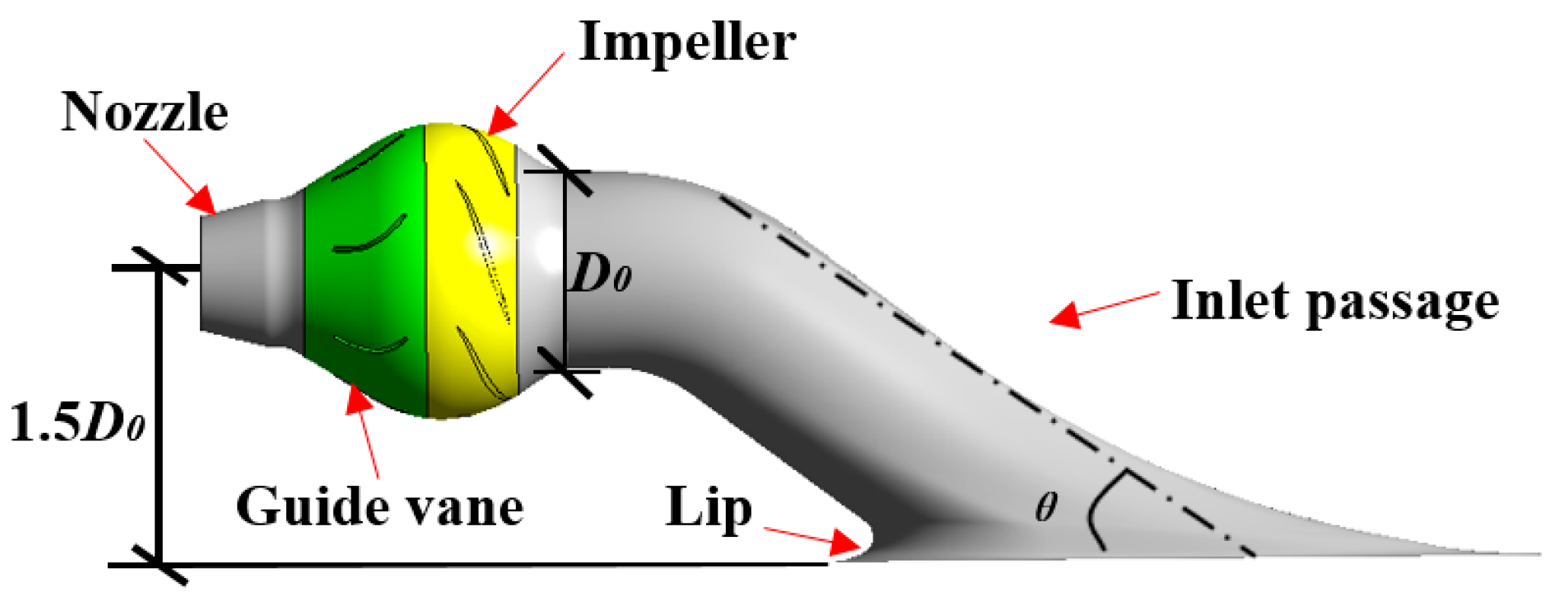
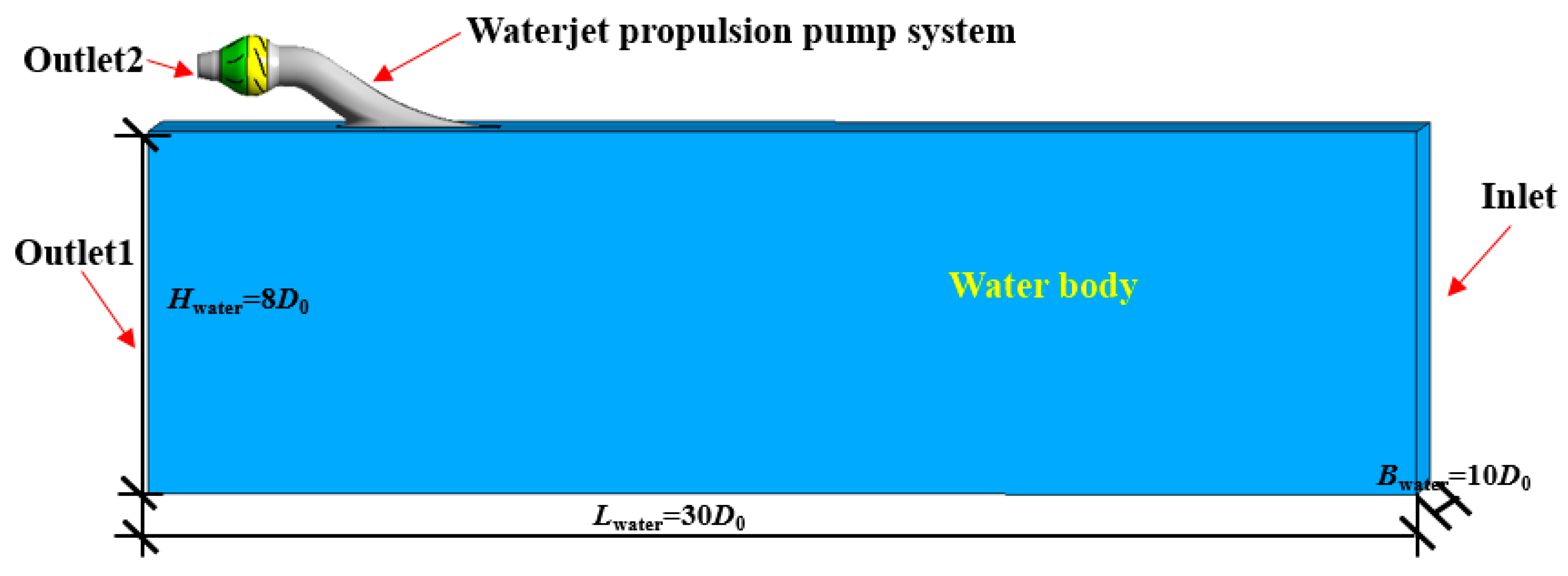
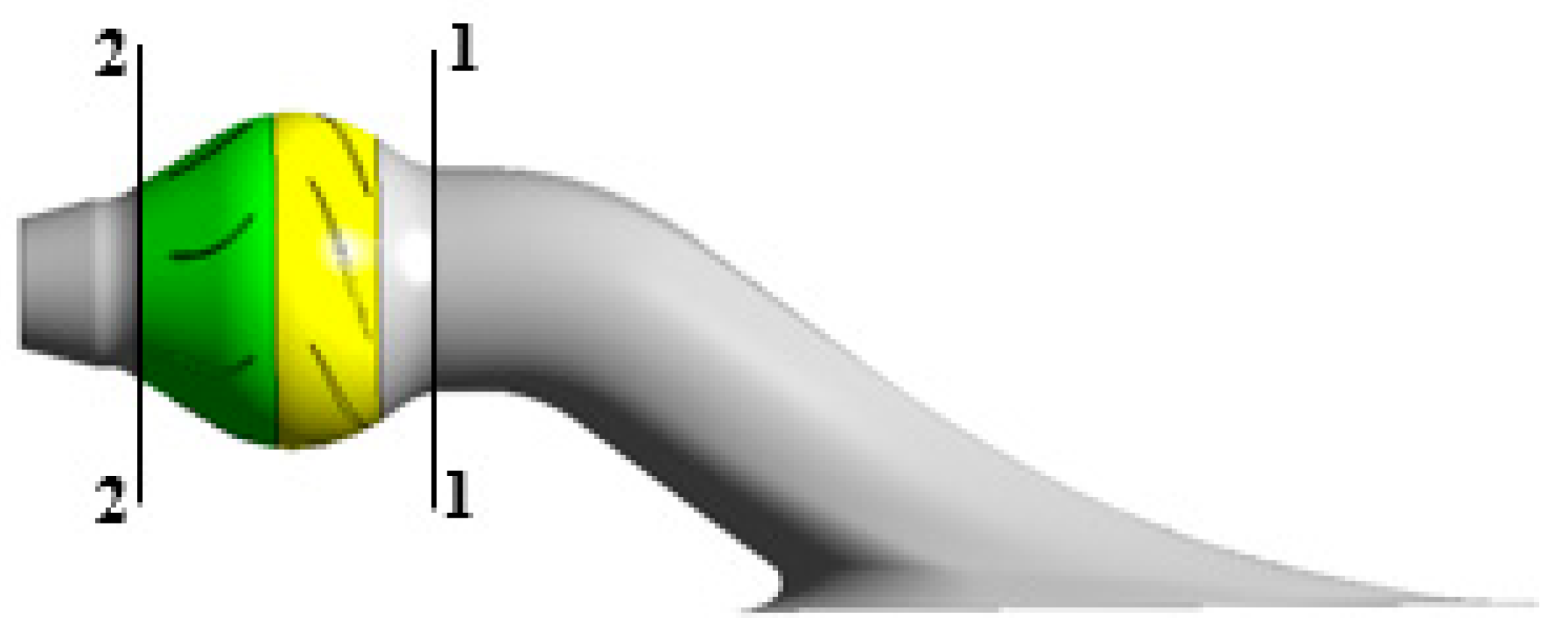
2.1. Numerical Model

Calculations are performed using the commercial code ANSYS CFX 14.5. ANSYS CFX uses the element-based finite volume method. The hull boundary layer, inflow velocity, and pressure affect the water flow. Thus, the water flow into the inlet duct is not uniform. The water around the inlet of the waterjet propulsion system should also be included in the computational domain. As shown in Figure 1 and Figure 2, the entire model includes the water body and waterjet propulsion pump system, composed of the inlet duct, propulsion pump, and nozzle. The propulsion pump consists of an impeller with six blades and a guide vane with seven vanes. The rotating speed of the impeller is 700 rpm. D₀ represents the inlet diameter of the impeller. θ represents the dip angle of the inlet duct.

2.2. Governing Equations

Reynolds-averaged N-S equation and continuity equation were selected to describe the 3D incompressible viscous flow. The continuity equation is as follows:

$$\frac{\partial \rho }{\partial t}+\frac{\partial (\rho u_j)}{\partial x_j}=0$$

(1)

The momentum conservation equation is as follows:

$$\frac{\partial \rho u_i}{\partial t}+\frac{\partial (\rho u_i{u}_j)}{\partial x_j}=-\frac{\partial p}{\partial x_i}+\frac{\partial }{\partial x_j}\left[\mu \left\{\frac{\partial u_i}{\partial x_j}+\frac{\partial u_j}{\partial x_i}-\frac{2}{3}\frac{\partial u_i}{\partial x_j}{\delta }_{ij}\right\}\right]+\frac{\partial }{\partial x_j}\left(-\rho u_i{u}_j\right)$$

(2)

where $\rho$ represents water density (in m³/s), $u_i$, $u_j$ represents velocity component of fluid in the i and j directions (in m/s), t represents time (in s), p represents pressure (in Pa), $F_i$ represents volume force component in the i direction(in N), $\mu$ represents dynamics viscosity coefficient, and $x_i$, $x_j$ represents coordinate component.

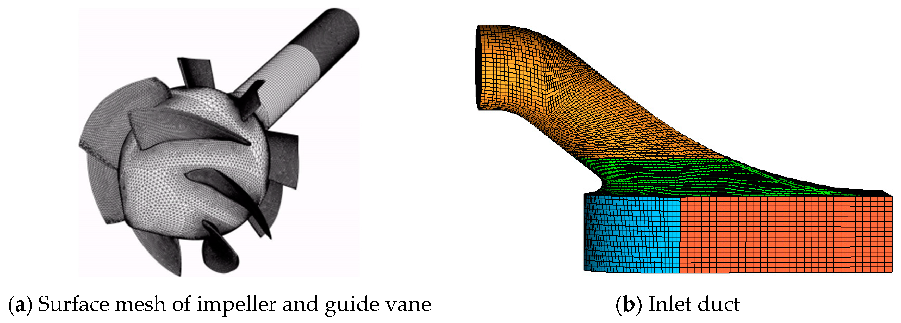
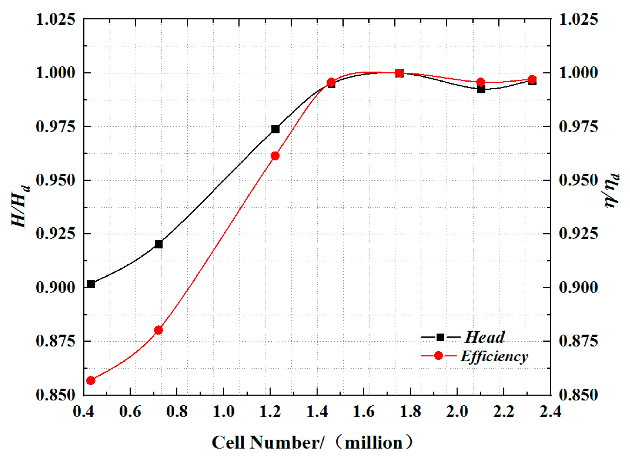
2.3. Grid Sensitivity Analysis

The computational domain consists of the water body, inlet duct, propulsion pump, and nozzle. The entire computational domain is generated with hexahedral grids and tetrahedral grids by ICEM software. An O-type grid of hexagonal cells was created around the impeller and stator blades by using an extrusion method to ensure good mesh quality in terms of size and skewness. The interior of the impeller and guide vane domain is filled with an unstructured mesh of tetrahedral cells because of the complex topology of the pump. The grid of the calculation domain is shown in Figure 3.

A grid sensitivity study was conducted to assess the required grid density. Several grid sizes were considered, ranging from a total number of cells of 4.3 × 10⁵ up to 2.1 × 10⁶. The standard k-ε is selected as the calculation model in this study. Hence, the y+ values are guaranteed to vary between 30 and 100 to satisfy the computational requirements while changing the grid density.

Figure 4 shows the mesh sensitivity analysis of the entire computational domain. The figure reveals that the efficiency and head of the waterjet propulsion pump system increase with the increase in the number of cells. When the number of cells reaches 1.5 million, the head and efficiency remain unchanged with the increase in the number of grids. Theoretically, with the increase in the number and density of grids, the calculation accuracy is generally improved. However, as the number of cells increases, the requirement for computer resources also increases, and the computing speed slows down. Therefore, the final cell number of the entire computational domain is 1,752,299. The y+ value of the propulsion pump is in the range of 30–100 in this study.

2.4. Turbulence Model Selecting

The turbulence model was introduced into the numerical calculation to solve the N-S equations. k-ε and k-ω are the commonly used turbulence models in calculation [35,36,37]. To select the most suitable turbulence model for calculation, this study used several different turbulence models, and the numerical results were compared with the experimental results.

Table 1. Numerical and experimental results with different turbulent models.

Turbulence Model	Standard k-ε	RNG k-ε	Standard k-ω	SST	SSG
H/Htd	1.0115	1.0263	1.0437	1.0655	1.0271
Efficiency η/ηtd	1.0237	1.0274	1.1088	1.1098	1.0341

H_td represents the test value of head under design flow rate condition. η_td represents the test value of pump efficiency under design flow rate condition.

presents the numerical and experimental results of different turbulence models under the operating conditions of 700 rpm. A slight difference was observed between the calculated values. However, under the condition of the standard k-ε turbulence model, the calculated values are in good agreement with the experimental values. Therefore, the standard k-ε is selected as the calculation model, and the scalable wall-function is used to improve robustness and accuracy.

2.5. Boundary Conditions

The inlet of the water body was set as the inlet boundary of the entire computational domain, and normal speed 8 m/s was adopted as the inlet boundary condition. The Reynolds number of the water body inlet is 4.19 × 10⁶. The inflow velocity is equal to ship speed, and nominal turbulence intensities (with a value equal to 5%) are used at the inlet boundary. The outlet of the water body and nozzle were set as the outlet boundary. An average static pressure outlet boundary condition is applied with 1 atm at the water body outlet, and the mass–flow rate was adopted as the outlet boundary of the nozzle. No-slip condition was applied at solid boundaries. The interfaces between the rotational impeller and static diffuser were set as the frozen stage condition. The convergence precision is set to 10⁻⁵.

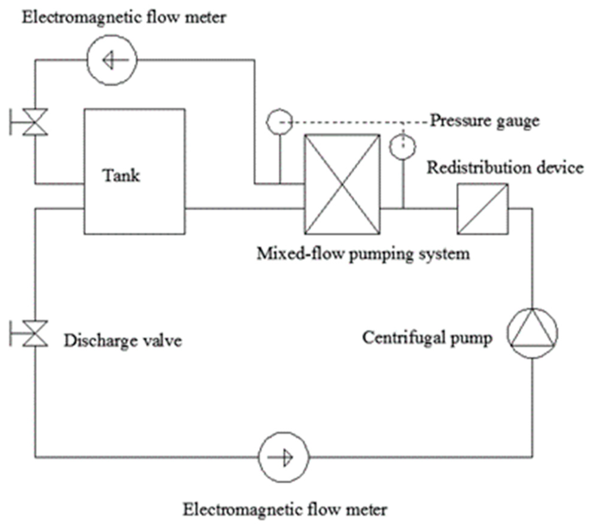
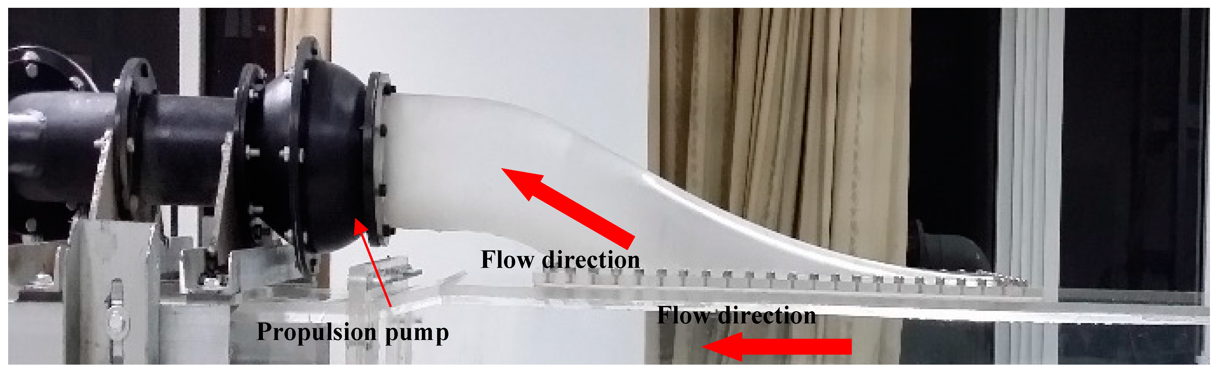
3. Hydraulic Characteristics Test

3.1. Test Rig Set-Up

A test rig is built, as shown in Figure 5, to study the hydraulic performance of the waterjet propulsion pump. The test rig is a closed circulation system that consists of two circulation pipeline systems: Main circulation pipeline and second circulation pipeline. The main circulation pipeline system is designed to ensure the water circulation of the test rig and provide the bottom speed. The second circulation pipeline system is the circulating pipe of the water jet propulsion pump, which is used to test the performance of the waterjet propulsion pump. The propulsion pumping system consists of a propulsion pump, a guide vane, and an inlet duct, as shown in Figure 6.

The propulsion pump with six impeller blades and the guide vane with seven stator vanes are built into the system. The scale model of a waterjet pump is used for ship propulsion. The head, flow rate, torque, and speed were tested to obtain the hydraulic performance of the waterjet propulsion pump. The pump is driven by a DC electromotor at speeds varying from 700 rev/min to 2400 rev/min and equipped with an auxiliary axial pump to regulate the flow rate. The test rig has two electromagnetic flowmeters with an absolute accuracy of ±0.5%. These flowmeters are used to test the flow rate of the main circulation pipeline system and the second circulation pipeline system. The head of the waterjet propulsion pump is measured by the differential pressure transmitter with an absolute accuracy of ±0.2%.

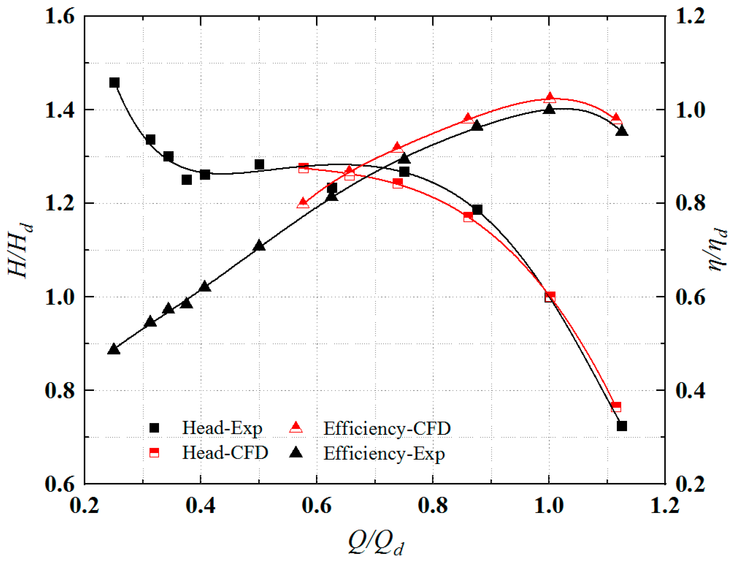
3.2. Experimental Verification

As shown in Figure 7, in the numerical calculation, the front section (1—1) of the impeller inlet and the back section of the guide vane outlet (2—2) were considered the pressure measuring sections for the head calculation and analysis.

The pump efficiency η, shaft power N, and head H were used to define the hydraulic characteristics of the waterjet propulsion pump system. The calculation formula is as follows:

$$P=P_{2-2}-P_{1-1}$$

(3)

$$H=\frac{P}{\rho g}$$

(4)

$$N=\frac{2\pi Tn}{1000\ast 60}$$

(5)

$$\eta =\frac{\rho gQH}{N}$$

(6)

where P is the pressure of the section (in Pa), $\rho$ is water density (in kg/m³), g is gravitational acceleration (in m/s²), T is the torque of blades (in N∙m), n is the rotating speed of the impeller (in r/min), Q is the flow rate (in m³/s), and N is the shaft power (in kW).

The comparative finding of the calculation and the experiment results reveals that the overall trend is similar, as shown in Figure 8. In general, the predicted H and η are in good agreement with the experiment results. Figure 8 shows that the difference between the experiment results and predicted results of H and η is minimum under the design flow-rate condition. In the numerical results, the performance of the head is better than that in the test results. At the design flow rate, the head difference between the test data and numerical data is 1.2%, and the efficiency difference between them is 2.4%. The findings show that the numerical results are reliable.

4. The Influence of Nozzle with Different Geometric Parameters on Hydraulic Characteristics of Waterjet Propulsion System

Conducting an in-depth study on the nozzle is necessary to further improve the hydraulic performance and waterjet propulsion efficiency of the waterjet propulsion system. Nine cases are designed to analyze the influence of nozzles with different geometric parameters on the waterjet propulsion system. As shown in

Table 2. Research cases.

Case	Shape	Area	Transition Curve Form	Note
				Diagram of Shape	Value
1	Circle	30%Ad	Linear contraction	Circle shape Elliptical shape Rounded rectangle	D1 = 0.55 D0
2	Elliptical	30%Ad	Linear contraction		a2 = 0.33 D0 b2 = 0.22 D0
3	Rounded rectangle	30%Ad	Linear contraction		c3 = 0.65 D0 d3 = 0.43 D0 r = 0.22 D0
4	Circle	10%Ad	Linear contraction		D1 = 0.32 D0
5	Circle	20%Ad	Linear contraction		D1 = 0.45 D0
6	Circle	40%Ad	Linear contraction		D1 = 0.63 D0
7	Circle	50%Ad	Linear contraction		D1 = 0.71 D0
8	Circle	30%Ad	Curve contraction followed by straight line		D1 = 0.55 D0
9	Circle	30%Ad	Arc contraction		D1 = 0.55 D0

A_d represents outlet area of the inlet duct.

, Cases 1–3 were selected to further investigate the influence of different nozzle outlet shapes on the hydraulic characteristics of the waterjet propulsion system. Case 1 and Cases 4–7 were selected to further investigate the influence of different nozzle outlet areas on the hydraulic characteristics of the waterjet propulsion system. Case 1 and Cases 8–9 were selected to further investigate the influence of different transition curve forms of the nozzle on the hydraulic characteristics of the waterjet propulsion system.

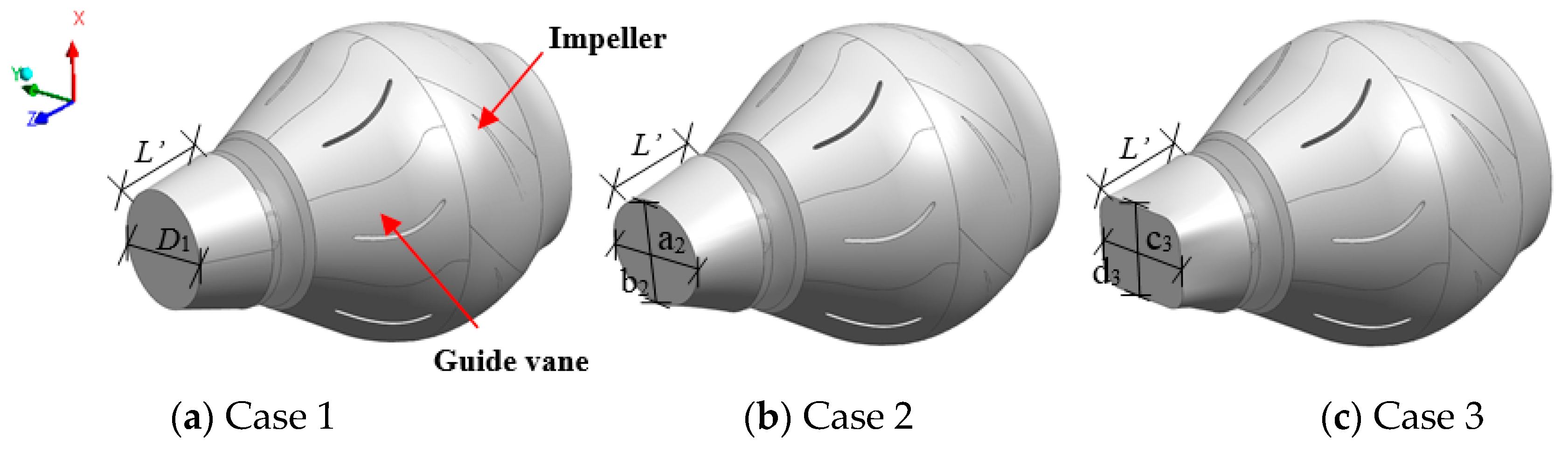
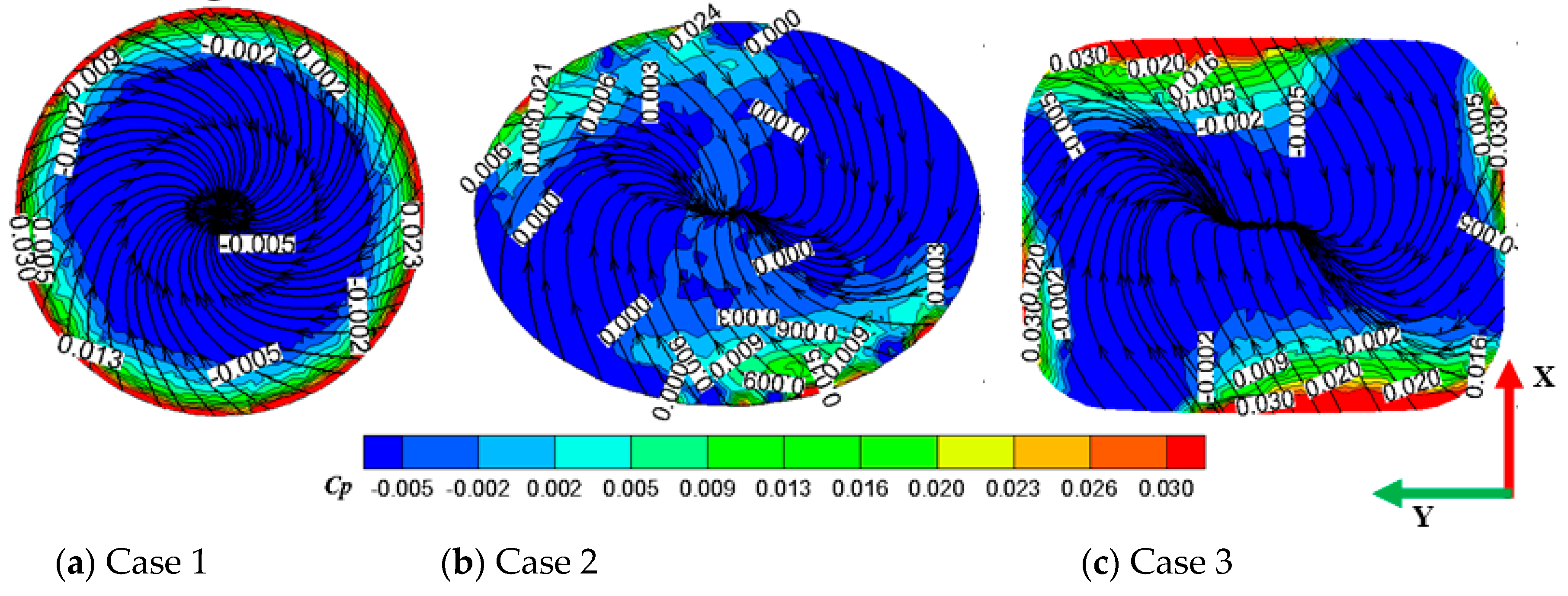
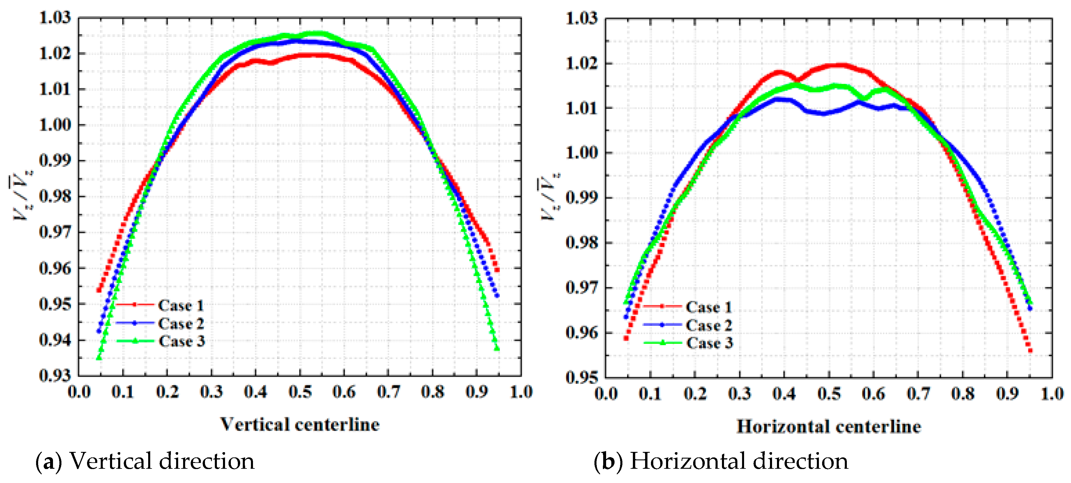
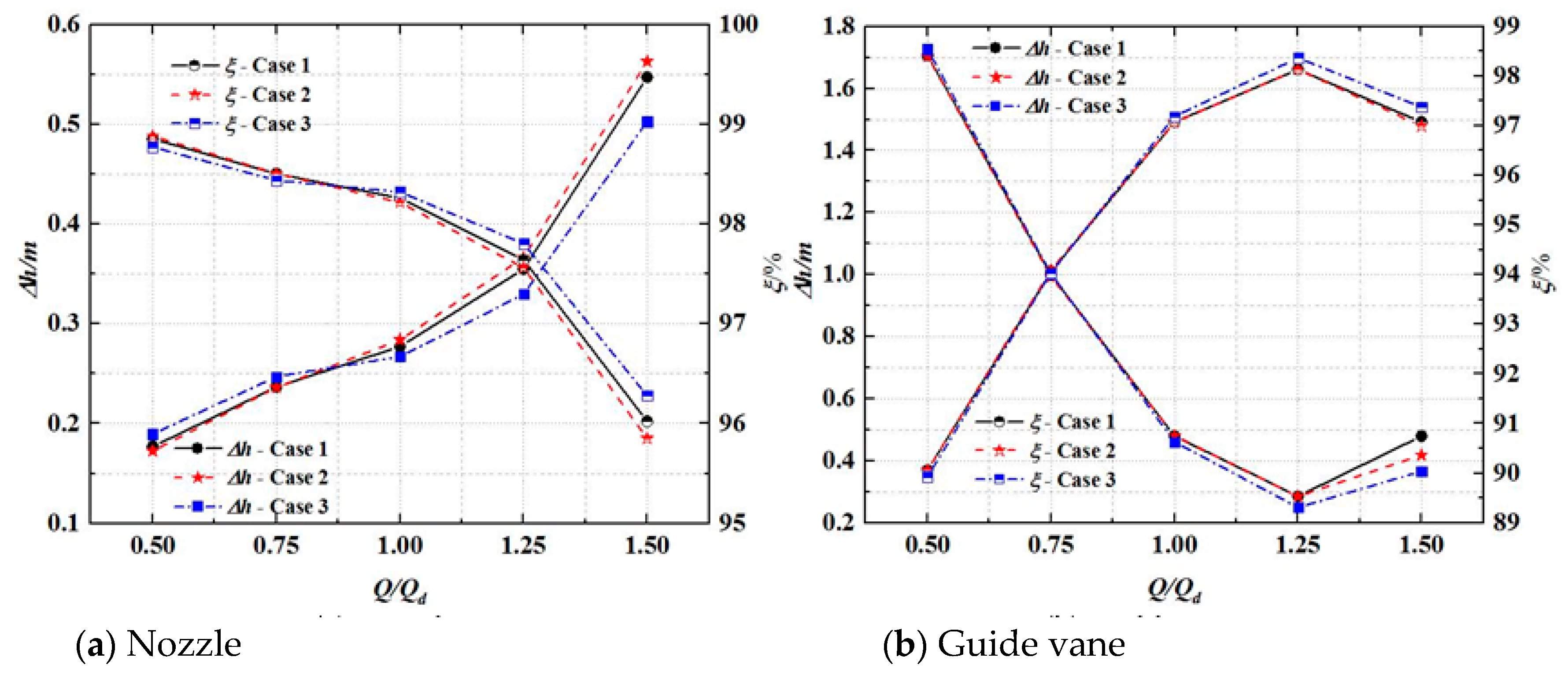
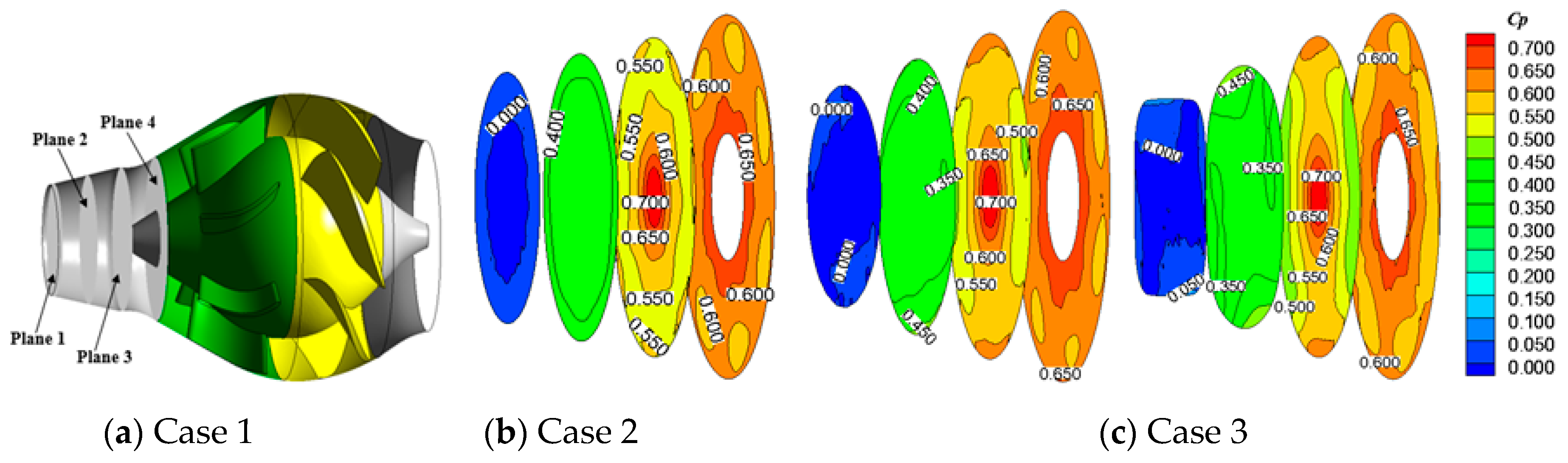
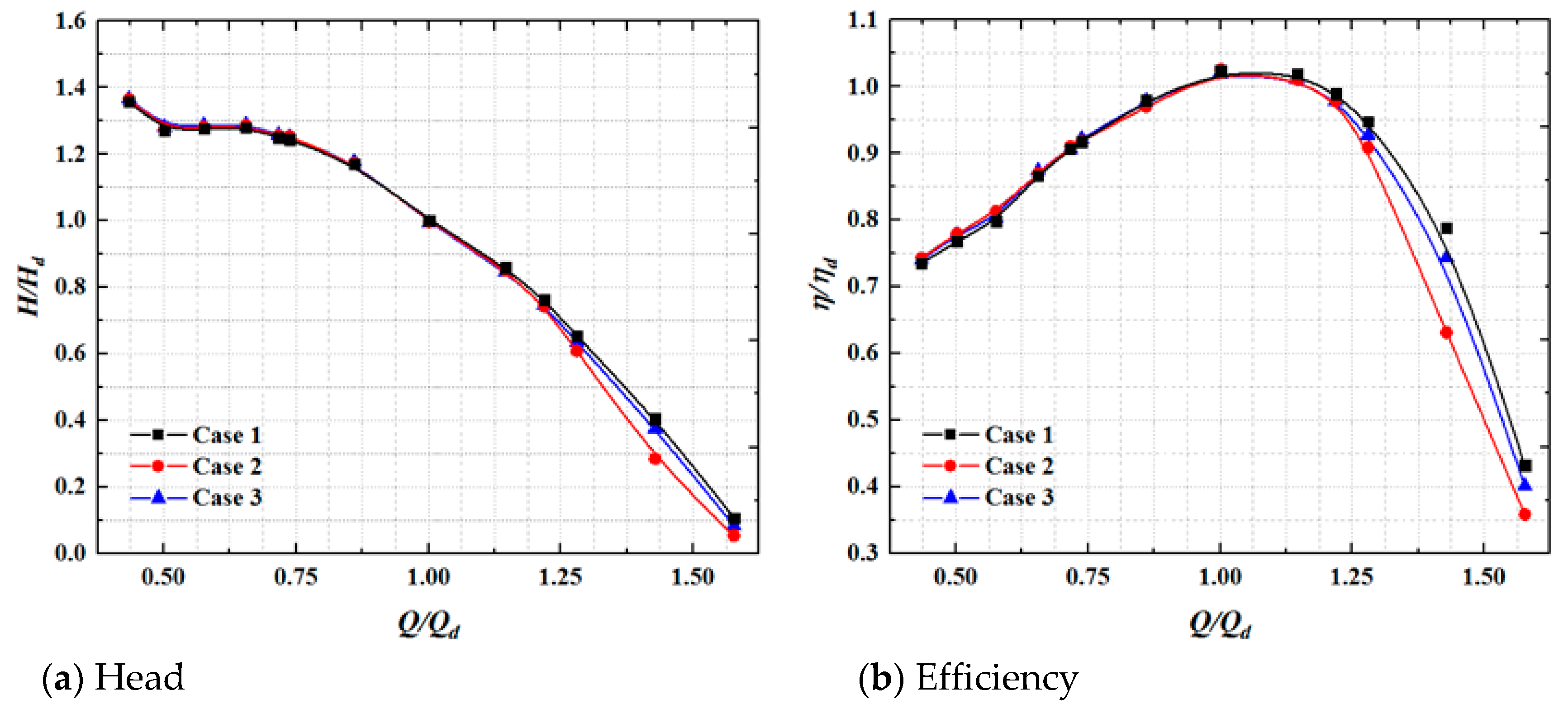
4.1. The Influence of Different Nozzle Outlet Shapes on the Hydraulic Characteristic

The nozzle with a circular shape was mostly used in practical applications, but whether the hydraulic performance of the circular nozzles is optimal remains unclear. Three different nozzle outlet shapes were set up for comparison, as shown in Figure 9, to explore the influence of different nozzle shapes on the hydraulic characteristics of the waterjet propulsion system. The nozzle outlet section shape is changed under the premise of maintaining a constant outlet area of the nozzle. The outlet section of the nozzle in Case 1 is circular, the outlet section of the nozzle in Case 2 is elliptical, and the outlet section of the nozzle in Case 2 is a rounded rectangle. All three outlet sections of different shapes have an area of 30% A_d. a and b denote the long axis and short axis of the elliptical outlet section, respectively. Meanwhile, a and b denote the width and height of the rounded rectangle outlet section. The ratio of a and b is 1.5.

The pressure coefficient $C_p$ is used to characterize the change of the nozzle outlet pressure. The pressure coefficient $C_p$ is a dimensionless value that describes the relative pressure throughout the flow field in fluid dynamics.

$$C_p=\frac{p-\overline{p}}{\frac{1}{2}\rho v_{out}{}^2}$$

(7)

where p is instantaneous pressure (in Pa), $\overline{p}$ is average pressure (in Pa), and v_out is averaged outlet velocity at the nozzle (in m/s).

Figure 10 presents the pressure contours and streamlined diagram of the nozzle outlet section with different nozzle shapes. As shown in Figure 10a, the pressure on the outlet of the circular nozzle is distributed uniformly as a ring. The pressure decreases uniformly from the circumference to the center of the circle. The streamline distribution shows that the flow lines on the outlet section intersect at the center of the circle, and the flow direction of the streamlines is consistent with the rotation direction of the impeller mainly because the guide vanes fail to completely recover the velocity loop. As shown in Figure 10b, the pressure distribution of the elliptical nozzle is relatively uneven. The pressure is symmetrically distributed diagonally. The flow direction of the streamlines is consistent with the direction of the rotation of the impeller. The intersection line of the streamlines at the center of the ellipse is curved. Figure 10c shows four high-pressure zones on the outlet section of the rounded rectangle nozzle. The high-pressure zone is mainly distributed at four rounded corners. The area of the high-pressure zones of the upper and lower side walls is larger than that of the left and right side walls. The flow direction of the streamlines is consistent with the direction of the rotation of the impeller. The intersection line of the streamlines at the center of the rounded rectangle is curved.

The uniformity of the velocity distribution at the nozzle outlet is represented by the axial velocity distribution coefficient $\overline{V}$. The axial velocity distribution is the best when the axial velocity distribution coefficient is close to 100%. The formula for the axial velocity distribution coefficient $\overline{V}$ is as follows:

$$\overline{V}=\left[1-\frac{1}{\overline{u_a}}\sqrt{\frac{{\displaystyle \sum {(u_{ai}-\overline{u_a})}^2}}{n}}\right]\times 100\%$$

(8)

where u_ai is the axial velocity of each element of the calculated section (in m/s), $\overline{u_a}$ is the averaged axial velocity of the calculated section (in m/s), and n is the number of cells of the calculated section.

The velocity uniformity of the three cases is 97.57%, 97.31%, and 97.23%. Different nozzle shapes provide a slight difference in the velocity distribution of the nozzle outlet section. Figure 11 shows the axial velocity distribution curve, and the data point coordinates are normalized. The axial velocity points were uniformly selected for the outlet sections of the three cases along the direction of the vertical and horizontal centerlines. Figure 11a shows the velocity curve along the vertical direction of the center of the outlet section. The vertical direction is the X-axis direction in Figure 10. The high-velocity zones of the three cases are concentrated in the outlet center. The axial velocity drops rapidly close to the upper and lower walls of the nozzle. The three curves show that the axial velocity curve of Case 1 changes more smoothly and evenly. Among the three cases, Case 3 has the greatest range of velocity variation, and the velocity at the center of the nozzle outlet has the largest difference from the velocity at the side wall. Figure 11b shows the velocity curve along the horizontal direction of the center of the outlet section. The horizontal direction is the Y-axis direction in Figure 10. The high-velocity zones of the three cases are concentrated in the outlet center. However, the velocity of the outlet center fluctuates greatly in the horizontal direction. In particular, because the section shrinkage of Cases 2 and 3 is not as uniform as that of Case 1, the velocity changes of Cases 2 and 3 fluctuate intensely. Among the three cases, Case 1 has the greatest range of velocity variation. However, the velocity curve of Case 1 is the most uniform and has a smooth curve. The velocity drops rapidly at the side wall because the velocity near the nozzle wall is very small. The velocity of the three cases in the Y-axis direction is not as uniform as that in the X-axis direction. In particular, the velocity fluctuates greatly near the center in the Y-axis direction.

The hydraulic performance of the nozzle and guide vane is measured by hydraulic loss. The pressure energy recovery coefficient is introduced to reflect the recovery of static pressure on the nozzle and guide vane. The formulas for the hydraulic loss $△h$ and pressure energy recovery coefficient $\xi$ are as follows:

$$△h=\frac{P_{in}-P_{out}}{\rho g}$$

(9)

$$\xi =\frac{P_{out}}{P_{in}}\times 100\%$$

(10)

where $P_{in}$ is the total pressure of the inlet section of the nozzle or guide vane (in Pa), and $P_{out}$ is the total pressure of the outlet section of the nozzle or guide vane (in Pa).

Figure 12 shows the relationship between the hydraulic loss and the pressure energy recovery coefficient of the nozzle and guide vane. As shown in Figure 12a, the hydraulic loss of the nozzle is small when the pressure energy recovery coefficient of the nozzle is large. The hydraulic loss and pressure energy recovery coefficients of Cases 1 and 2 are nearly identical when the flow rate is 0.5 to 0.75 times the design flow rate. The hydraulic loss of Case 3 is larger than that of Cases 1 and 2, and the pressure energy recovery coefficient is smaller than that of Cases 1 and 2. The increase in the hydraulic loss of Case 3 is slower when the flow rate is 0.75 to 1 time the design flow rate, initially larger than that of Cases 1 and 2, and then gradually smaller than that of Cases 1 and 2. The pressure energy recovery coefficient of Case 3 is smaller than that of Cases 1 and 2, and then larger than that of Cases 1 and 2. Under the design flow rate condition, the pressure energy recovery coefficient of Case 3 is the largest, and the hydraulic loss is the smallest. The pressure energy recovery coefficient of Case 2 is minimum. At this time, the pressure recovery coefficients of Cases 1, 2, and 3 are 98.26%, 98.21%, and 98.32%, respectively. When the flow rate is greater than the designed flow rate, the pressure recovery performance of Case 3 is better than that of Cases 1 and 2. Thus, the hydraulic loss of Case 3 is smaller than that of Cases 1 and 2. When the flow rate is greater than 1.25 times the designed flow rate, the hydraulic loss of the three cases decreases more severely with the increase in the flow rate. When the flow rate is 1.5 times the designed flow rate, the pressure energy recovery coefficient of Case 3 is 0.26% and 0.43% higher than that of Cases 1 and 2, respectively. As shown in Figure 12b, the relationship between the pressure energy recovery coefficient and hydraulic loss of the guide vane is opposite to that of the nozzle. In addition, the relationship between the pressure energy recovery coefficient (and the hydraulic loss) and the flow rate of the guide vanes is not a monotonic function. The pressure energy recovery coefficient of the guide vane initially increases and then decreases with the increase in the flow rate. The hydraulic loss of the guide vane initially decreases and then increases with the increase in the flow rate. When the flow rate is 1.25 times the designed flow rate, the hydraulic loss of the guide vanes of the three cases reaches the maximum, and the pressure energy recovery coefficient is the smallest. Figure 12a,b shows that when the pressure recovery of the guide vane is worse, the pressure recovery of the nozzle is better. Under the conditions of small flow rate and designed flow rate, the difference between the pressure recovery coefficient and hydraulic loss of nozzles and guide vanes in the three cases is extremely small. Under large flow rate conditions, the pressure energy recovery coefficient and hydraulic loss of Case 3 are optimal, and those of Case 2 are the worst.

Figure 13 shows the distributions of the pressure contours of the longitudinal section of the nozzles. Four longitudinal sections are intercepted equidistantly in the nozzle. As illustrated in the figure, seven high-pressure zones due to the influence of guide vane are shown in Plane 4. Compared with the three results, the change in the shape of the nozzle affects the pressure distribution at the nozzle. In Case 1, as the section approaches the outlet of the nozzle, the pressure distribution in the section becomes increasingly uniform. The pressure distribution in Case 3 is the most uneven. In the three cases, the pressure distribution near the outlet is similar to the shape of the outlet section.

Figure 14 shows the comparison of the hydraulic performance of different nozzle shapes. The figure shows that the trend of the head and efficiency curves of the three cases is consistent. The head initially decreases and then increases with the increase in the flow rate, and then continues to decrease. The head increases with the flow rate when the flow rate is 0.5 to 0.75 times the designed flow rate. The efficiency initially increases and then decreases with the increase in the flow rate. It has the highest efficiency point. The corresponding flow rate of the high-efficiency area is (1.0–1.2) Q_d. When the flow reaches (0.42–1.2) Q_d, the flow and head curves of the three cases are almost coincident. Each performance value is higher near the design flow range. The head and efficiency are lower when the flow rate is larger than the designed flow rate. The head and efficiency of Cases 2 and 3 are lower than those of Case 1. When the flow rate is larger than 1.25 times the designed flow rate, the head and efficiency curves of Case 2 drop rapidly because the elliptical nozzle is more irregular and shrinks more sharply than those in the other two cases.

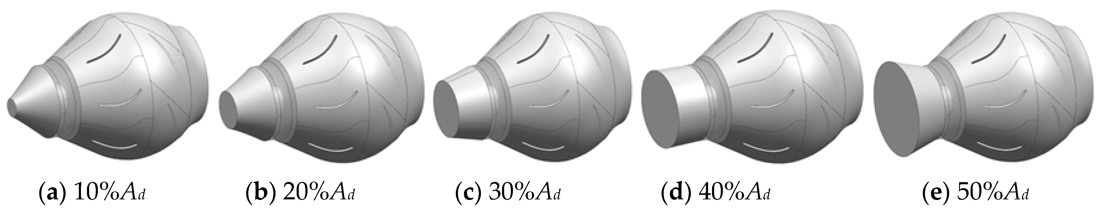
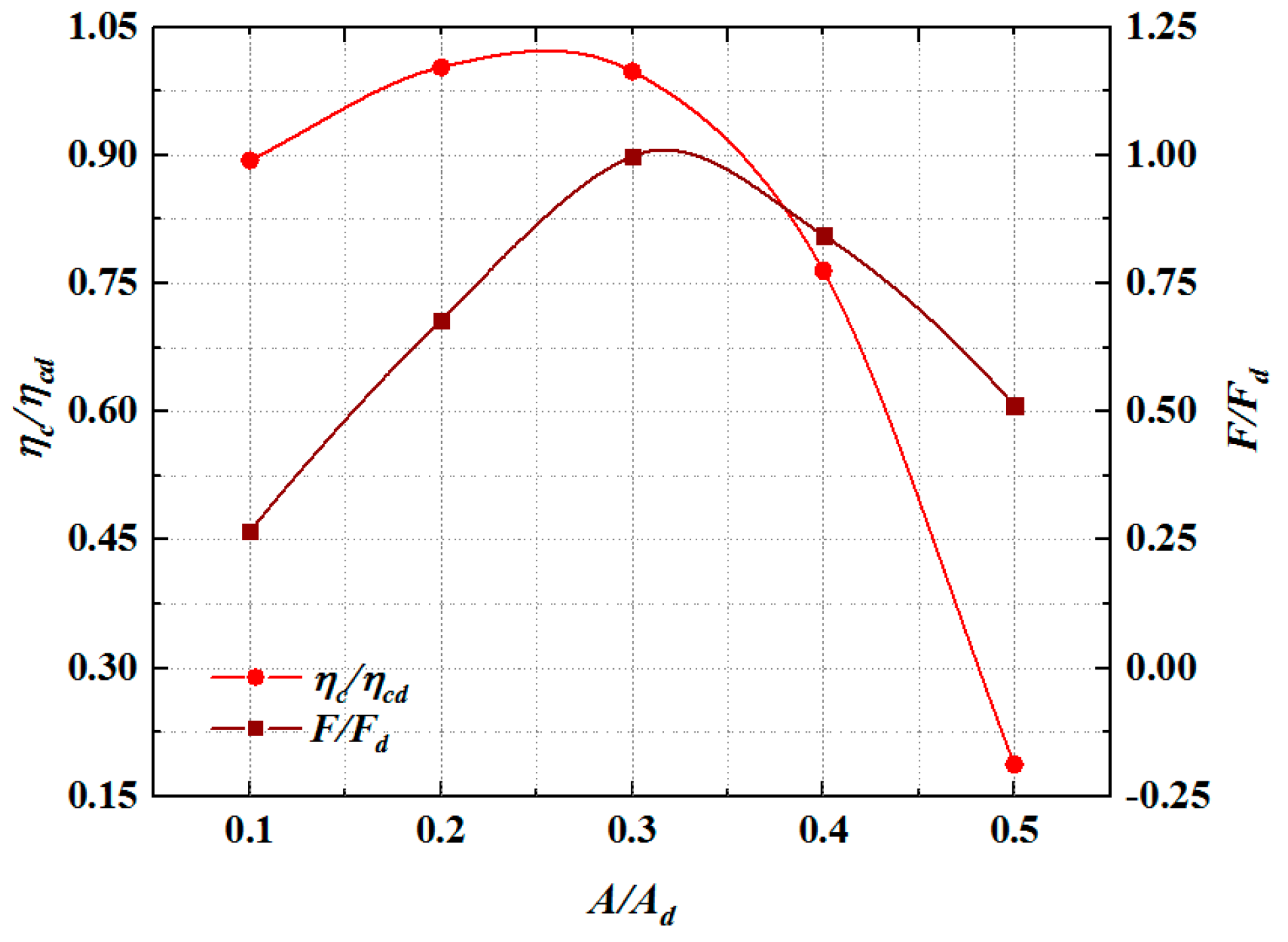
4.2. The Influence of Different Nozzle Outlet Areas on the Hydraulic Characteristic

Figure 15 shows the 3D diagram of the circular nozzle with different outlet areas. The hydraulic characteristics of the waterjet propulsion pump system are better when the circular nozzle is used. The hydraulic characteristics of different outlet areas of the nozzle were studied under the condition of the circular nozzle. The hydraulic characteristics of the waterjet propulsion systems with five different nozzle areas were studied. The nozzle area varies from 10% to 50% times the outlet area of the inlet duct.

Figure 16 shows the pump efficiency, head, shaft power, and IVR (Inlet Velocity Ratio) curves of the waterjet propulsion pump system with different outlet areas of the nozzle. IVR refers to the ratio of the ship speed to the averaged axial outflow velocity at the duct outlet. The averaged axial outflow velocity at the duct outlet is an important parameter to describe the flow phenomena in the inlet, where the speed is changed from the ship speed to the pump velocity. IVR is defined as follows:

$$IVR=\frac{v_{duct}}{v_s}$$

(11)

where $v_{duct}$ is the averaged axial outflow velocity at the duct outlet (in m/s), and $v_s$ is the ship speed (in m/s).

Figure 16a presents the relationship between efficiency and head with the nozzle area. The head decreases and efficiency initially increases and then decreases with the increase in the nozzle area. The head decreases slowly when the nozzle outlet area changes from 10% A_d to 30% A_d. From the curve, the head drops from 1.14 H_d to 1.0 H_d. Meanwhile, the efficiency curve increases, and the efficiency rises from 0.53 η_d to 1.0 η_d. When the nozzle area exceeds 30% A_d, the head curve drops rapidly, and the efficiency curve begins to decline. When the nozzle outlet area changes from 30% A_d to 50% A_d, the head drops from 1.0 H_d to 0.36 H_d, and the efficiency is reduced from 1.0 η_d to 0.67 η_d. The best efficiency point is obtained when the outlet area is near 30% A_d. Figure 16b shows the relationship between power and IVR with the nozzle area. With the increase in the nozzle outlet area, IVR increases, and the power initially increases and then decreases. When the nozzle outlet area changes from 10% A_d to 30% A_d, IVR rises from 0.32 IVR_d to 1.0 IVR_d, and the shaft power rises from 0.69 N_d to 1.0 N_d. When the nozzle outlet area changes from 30% A_d to 50% A_d, the IVR curve rises slowly from 1.0 IVR_d to 1.37 IVR_d. When the nozzle outlet area exceeds 30%A_d, the power curve no longer rises and begins to fall. The maximum power point is obtained when the outlet area is near 30%A_d. Therefore, the maximum efficiency and shaft power occur when the nozzle outlet area is 30% A_d, and the hydraulic characteristics of the waterjet propulsion pump system are better.

The purpose of the waterjet propulsion system is to produce thrust to propel a ship. To study the influence of the nozzle outlet area on the waterjet propulsion system, this study considers two important factors, namely, thrust and system efficiency, in addition to the performance curves.

The thrust of the waterjet propulsion system is defined, considering the influence of the boundary, as follows:

$$T=\rho Q(v_{out}-v_{in})$$

(12)

$$v_{in}=\alpha v_s$$

(13)

$$Q=A{v}_{out}$$

(14)

where A is the outlet area of the nozzle, $v_{in}$ is the mass-averaged ingested velocity at the duct inlet, and $\alpha$ is the effect coefficient of the boundary layer, which is 0.95 according to the reference documentation.

The efficiency of the waterjet propulsion system ${\eta }_c$ denotes the ratio of the output power of the system to that of the propulsion pump. Considering the pipeline loss coefficient, the formula for the ${\eta }_c$ is as follows:

$${\eta }_c=\frac{2(k-\alpha )}{k{\prime }^2-\beta +K_1}$$

(15)

$$\beta ={\alpha }^2$$

(16)

where K₁ is the pipeline loss coefficient in the range of 0.40–0.50. In this study, K₁ is 0.45, k’ is the ratio of $v_{out}$ to $v_s$ vs, and β is the effect coefficient of the boundary layer.

Figure 17 shows the system efficiency and thrust curves of the waterjet propulsion system with different nozzle outlet areas. The thrust and system efficiency of the waterjet propulsion system initially increase and then decrease with the increase in the outlet area. When the nozzle outlet area changes from 10% A_d to 30% A_d, the thrust rises from 0.27 F_d to 1.0 F_d, and the system efficiency rises from 0.89 η_cd to 1.0 η_cd. When the nozzle outlet area exceeds 30% A_d, the thrust and system efficiency curves no longer rise and begin to fall. When the nozzle outlet area changes from 30% A_d to 50% A_d, the thrust reduces from 1.0 F_d to 0.51 F_d, and the system efficiency declines from 1.0 η_cd to 0.19 η_cd. The maximum system efficiency and thrust are obtained when the outlet area is close to 30% A_d. The nozzle area greatly influences the thrust. When the outlet area exceeds 30% A_d, the system efficiency curve decreases rapidly. When the nozzle outlet area is extremely large, the nozzle diffuses the water flow. Thus, the axial velocity of the nozzle outlet v_out is less than the velocity of the inlet section of the inlet duct v_in, and the thrust value is negative.

4.3. The Effect of Different Transition Curve Forms on the Hydraulic Characteristic

Figure 18 shows the transition curve forms of the nozzle. The first component is the nozzle, and the second component is the guide vane outlet. The total length of the nozzle and outlet section of the guide vane L’, guide vane outlet diameter D_g, nozzle outlet diameter D₁, and shrinkage arc radius of the guide vane outlet section R₁ are constant. In Cases 1, 8, and 9, the transition curve forms of the nozzle were changed. In Case 1, the linear contraction is selected as the transition curve form. The shrinkage angle $\theta \prime$ of the nozzle with linear contraction is 13°. In Case 8, the combined contraction of the curve and the straight line is selected as the transition curve form. The curve segment consists of arc segments with radii R2 and R3. In Case 9, the arc contraction is selected as the transition curve form. The geometric parameters of the nozzle are shown in

Table 3. Geometric parameters of the nozzles with different contraction curves.

Case	L’	D1	Dg	R1	θ	R2	R3	R4
1	0.56D0	0.55D0	0.86D0	0.37D0	13°	/	/	/
8	0.56D0	0.55D0	0.86D0	0.37D0	/	0.30D0	0.11D0	/
9	0.56D0	0.55D0	0.86D0	0.37D0	/	/	/	0.87D0

.

Figure 19 shows the ratio of the hydraulic performance of the three types of transition curves to that of Case 1. The thrust value is the axial thrust from the inlet duct to the nozzle section. The figure indicates that the system efficiency and thrust of the system corresponding to Case 1 are the greatest for the three types of nozzles, but their values are similar to those of Case 8. The main reason is that the hydraulic losses of the two types of nozzles are relatively small. The hydraulic losses of Case 9 are larger than those of the others given the excessive contraction at the nozzle.

The ideal nozzle outflow condition is that the outlet water flow angle is perpendicular to the nozzle outlet section. Thus, the mechanical energy of the propulsion pump can be maximally converted into the kinetic energy of the water. The outlet water flow cannot be completely perpendicular to the nozzle outlet section due to the tangential velocity of the nozzle outlet. Thus, the weighted-velocity average swirl angle $\overline{\theta }$ is used to measure the outflow conditions of the nozzle. The outlet water flow angle perpendicular to the nozzle outlet section is better when $\overline{\theta }$ is closer to 90°. The formula for velocity-weighted average swirl angle $\overline{\theta }$ is as follows:

$$\overline{\theta }=\frac{{\displaystyle \sum _{i=1}^n\left[v_{ai}\left(90-\arctan \frac{v_{ui}}{v_{ai}}\right)\right]}}{{\displaystyle \sum _{i=1}^n{v}_{ai}}}$$

(17)

where u_ti is the tangential velocity of each element of the calculated section (in m/s), and u_ai is the axial velocity of each element of the calculated section (in m/s).

Table 4. Hydraulic performance of the nozzle with different contraction curves.

Case	${\mathit{v}}_{\mathbf{max}}(\mathbf{m}/\mathbf{s})$	$\overline{\mathit{v}}(\mathbf{m}/\mathbf{s})$	$\overline{\mathit{V}}$	$\overline{\mathit{\theta }}$
1	10.42	10.02	97.57%	78.73°
8	10.47	9.78	94.24%	80.10°
9	10.44	9.81	96.07%	75.07°

shows the hydraulic performance of the nozzle with different contraction curves. $v_{\max }$ denotes the maximum axial outlet velocity of the nozzle, $\overline{v}$ denotes the averaged outlet axial velocity of the nozzle, $\overline{V}$ denotes the axial velocity distribution coefficient, and $\overline{\theta }$ denotes the velocity-weighted average swirl angle.

As shown in Table 4, the maximum axial velocity values of the nozzle outlet section of the three cases are basically the same. Therefore, the three cases have good shrinkage effects. The comparative result of the average axial velocity of the three cases shows that the average axial velocity of Case 1 is much larger than that of Cases 2 and 3. The average axial velocity of Case 1 is 1.025 and 1.021 times that of Cases 2 and 3, respectively. The comparative result of the axial velocity distribution coefficient of the three cases shows that the axial velocity distribution coefficient of Case 1 is the best. The axial velocity distribution uniformity of Case 1 is 3.33% and 1.5% more than that of Cases 2 and 3. The velocity-weighted average swirl angle of Case 2 is 80.1°, which is 1.37° and 5.03° higher than that of Cases 1 and 3, respectively. The velocity-weighted average swirl angle of Case 2 is the best mainly due to the rectification effect of the straight section before the outlet of the nozzle in Case 2.

Figure 20 shows the axial velocity contours and streamlines of the nozzle outlet section with different contraction curves. The figure shows that the axial velocity of the three cases is distributed in a ring-like manner, and the high-speed zone is concentrated at the center of the circle. The area of the high-speed zone in Cases 2 and 3 is larger, but the axial velocity distribution uniformity of Case 1 is better. The streamline distribution indicates that Case 2 is more affected by the straight section of the outlet of the nozzle, and the flow lines on the outlet section are more deflected.

5. Conclusions

In this study, the hydraulic characteristics of the nozzle of the waterjet propulsion system were studied by a combination of numerical simulation and experimental verification. Different grid values and turbulence models were used for calculation and analysis to determine the appropriate numerical settings and ensure the accuracy of the calculation. The model test was used to verify the external characteristics of the waterjet propulsion pump, and the numerical results are in good agreement with the test results. Therefore, the numerical results are reliable. Nine different cases were established to systematically study the hydraulic characteristics of the nozzle in accordance with the different nozzle outlet shapes, nozzle outlet areas, and nozzle transition curves. The following results are obtained through calculation and analysis:

(1) The pressure coefficient Cp, axial velocity distribution coefficient $\overline{V}$, hydraulic loss $△h$, and pressure energy recovery coefficient $\xi$ were introduced to analyze the hydraulic characteristics of the waterjet propulsion system with different nozzle outlet shapes. The outlet section pressure and streamline the distribution of the circular nozzle case is superior to those in the other two cases. The pressure on the outlet of the circular nozzle is distributed uniformly as a ring, and the flow lines on the outlet section intersect at the center of the circle. Under the design flow-rate condition, the velocity uniformity of the circular nozzle is 0.26% and 0.34% higher than that of the elliptical nozzle and the rounded rectangle nozzle, respectively. The pump efficiency of the circular nozzle is 0.31% and 0.14% higher than that of the others. At this point, the pressure recovery and hydraulic loss of the circular nozzle are superior. Under large flow-rate conditions, the pressure recovery and hydraulic loss of the rounded rectangle nozzle are superior to those in the other two cases. The external characteristic curves show that the circular nozzle case is better. The hydraulic performance of the elliptical nozzle is lower because the elliptical section is more irregular and shrinks more sharply than the other two sections.

(2) The comprehensive hydraulic characteristics are analyzed in accordance with the different nozzle outlet areas, waterjet propulsion pumps, and waterjet propulsion systems. The analysis of the hydraulic performance of the waterjet propulsion pump reveals that when the nozzle outlet area is close to 30% A_d, the waterjet propulsion system has the highest efficiency and the best hydraulic performance. When the nozzle area exceeds 30% A_d, the head curve descends faster and the IVR curve ascends slowly. The analysis of the hydraulic performance of the waterjet propulsion system reveals that when the outlet area is close to 30% A_d, the thrust and system efficiency reach the maximum value. When the outlet area exceeds 30% A_d, the system efficiency curve decreases rapidly.

(3) The comparison among different transition curve forms of the nozzle shows that the transition curve forms greatly affect the thrust and system efficiency. The linear contraction of Case 1 slightly affects the hydraulic performance of the nozzle mainly because the transition of the linear contraction is more uniform with less hydraulic loss. The average axial velocity and axial velocity distribution uniformity of Case 1 are better than those of the other cases. The velocity-weighted average swirl angle of Case 2 is optimal, but the hydraulic characteristics of Cases 2 and 3 are not as good as those of Case 1.

References

1. Bulten, N.W.H. Numerical Analysis of a Waterjet Propulsion System. Ph.D. Thesis, Library Eindhoven University of Technology, Eindhoven, Netherlands, 2006. [Google Scholar]
2. Takai, T.; Kandasamy, M.; Stern, F. Verification and validation study of URANS simulations for an axial waterjet propelled large high-speed ship. J. Mar. Sci. Technol. 2011, 16, 434–447. [Google Scholar] [CrossRef]
3. Lavis, D.R.; Forstell, B.G.; Purnell, J.G. Compact waterjets for high-speed ships. Ships Offshore Struct. 2007, 2, 11. [Google Scholar] [CrossRef]
4. Hu, B.; Li, X.; Fu, Y.; Zhang, F.; Gu, C.; Ren, X.; Wang, C. Experimental investigation on the flow and flow-rotor heat transfer in a rotor-stator spinning disk reactor. Appl. Therm. Eng. 2019, 162, 114316. [Google Scholar] [CrossRef]
5. Zhu, Y.; Qian, P.; Tang, S.; Jiang, W.; Li, W.; Zhao, J. Amplitude-frequency characteristics analysis for vertical vibration of hydraulic AGC system under nonlinear action. AIP Adv. 2019, 9, 035019. [Google Scholar] [CrossRef] [Green Version]
6. Verbeek, R.; Bulten, N.W.H. Recent development in waterjet design. In Proceedings of the International Conference on Waterjet Propulsion, Latest Developments, Amsterdam, The Netherlands, 22–23 October 1998; RINA: Amsterdam, The Netherlands, 1998. [Google Scholar]
7. Jiao, W.X.; Cheng, L.; Xu, J.; Wang, C. Numerical analysis of two-phase flow in the cavitation process of a waterjet propulsion pump system. Processes 2019, 7, 690. [Google Scholar] [CrossRef] [Green Version]
8. Ding, J.M.; Wang, Y.S. Research on flow loss of inlet duct of marine waterjets. J. Shanghai Jiaotong Univ. (Sci.) 2010, 15, 158–162. [Google Scholar] [CrossRef]
9. Park, W.G.; Yun, H.S.; Chun, H.H.; Kim, M.C. Numerical flow simulation of flush type intake duct of waterjet. Ocean Eng. 2005, 32, 2107–2120. [Google Scholar] [CrossRef]
10. Cao, P.; Wang, Y.; Li, G.; Cui, Y.; Yin, G. Numerical hydraulic efficiency analysis of waterjet propulsion. In Proceedings of the International Symposium on Fluid Machinery & Fluid Engineering, Wuhan, China, 22–25 October 2014. [Google Scholar]
11. Cheng, L.; Qi, W. Rotating stall region of water-jet pump. Trans. Famena 2014, 38, 31–40. [Google Scholar]
12. Xia, C.Z.; Cheng, L.; Luo, C.; Jiao, W.; Zhang, D. Hydraulic characteristics and measurement of rotating stall suppression in a waterjet propulsion system. Trans. Famena 2018, 4, 85–100. [Google Scholar] [CrossRef]
13. Wang, C.; He, X.; Zhang, D.; Hu, B.; Shi, W. Numerical and experimental study of the self-priming process of a multistage self-priming centrifugal pump. Int. J. Energy Res. 2019, 43, 4074–4092. [Google Scholar] [CrossRef]
14. Wang, C.; Shi, W.; Wang, X.; Jiang, X.; Yang, Y.; Li, W.; Zhou, L. Optimal design of multistage centrifugal pump based on the combined energy loss model and computational fluid dynamics. Appl. Energy 2017, 187, 10–26. [Google Scholar] [CrossRef]
15. Kim, M.C.; Chun, H.H. Experimental investigation into the performance of the Axial-Flow-Type Waterjet according to the Variation of Impeller Tip Clearance. Ocean Eng. 2007, 34, 275–283. [Google Scholar] [CrossRef]
16. Etter, R.J.; Krishnamoorthy, V.; Sherer, J.O. Model testing of waterjet propelled craft. In Proceedings of the 19th ATTC, Ann Arbor, American, 11–15 August 1980. [Google Scholar]
17. Eslamdoost, A.; Larsson, L.; Bensow, R. Net and gross thrust in waterjet propulsion. J. Ship Res. 2016, 60, 1–14. [Google Scholar] [CrossRef]
18. Park, W.G.; Jang, J.H.; Chun, H.H.; Kim, M.C. Numerical flow and performance analysis of waterjet propulsion system. Ocean Eng. 2005, 32, 1740–1761. [Google Scholar] [CrossRef]
19. Liang, J.; Li, X.; Zhang, Z.; Luo, X.; Zhu, Y. Numerical investigation into effects on momentum thrust by nozzle’s geometric parameters in water jet propulsion system of autonomous underwater vehicles. Ocean Eng. 2016, 123, 327–345. [Google Scholar]
20. Abcand, L.; Cobolli, C.R. Optimization of waterjet propulsion for high-speed ships. J. Hydronaut. 1968, 2, 2–8. [Google Scholar] [CrossRef]
21. Chin, P.C. Determination of the main parameters of water-jet propulsion system. Shipbuild. China 1978, 1, 80–91. [Google Scholar]
22. Jiao, W.X.; Cheng, L.; Zhang, D.; Zhang, B.; Su, Y.; Wang, C. Optimal design of inlet passage for waterjet propulsion system based on flow and geometric parameters. Adv. Mater. Sci. Eng. 2019, 2320981. [Google Scholar] [CrossRef] [Green Version]
23. Xin, B.; Luo, X.; Shi, Z.; Zhu, Y. A vectored water jet propulsion method for autonomous underwater vehicles. Ocean Eng. 2013, 74, 133–140. [Google Scholar] [CrossRef]
24. Gong, Z.H.; Li, G.Q.; Xiong, W.; Li, J.Z.; Yu, Y.X.; Yuan, J.Q. Modeling and Simulation of the Steering Control System of Marine Water-Jet Propulsion Unit. J. Shanghai Jiaotong Univ. 2016, 50, 1114–1118. [Google Scholar]
25. Wang, C.; He, X.; Shi, W.; Wang, X.; Wang, X.; Qiu, N. Numerical study on pressure fluctuation of a multistage centrifugal pump based on whole flow field. AIP Adv. 2019, 9, 035118. [Google Scholar] [CrossRef] [Green Version]
26. Zhu, Y.; Tang, S.; Quan, L.; Jiang, W.; Zhou, L. Extraction method for signal effective component based on extreme-point symmetric mode decomposition and Kullback-Leibler divergence. J. Braz. Soc. Mech. Sci. Eng. 2019, 41, 100. [Google Scholar] [CrossRef]
27. Wang, C.; Chen, X.; Qiu, N.; Zhu, Y.; Shi, W. Numerical and experimental study on the pressure fluctuation, vibration, and noise of multistage pump with radial diffuser. J. Braz. Soc. Mech. Sci. Eng. 2018, 40, 481. [Google Scholar] [CrossRef]
28. Wei, Y.; Yang, H.; Dou, H.S.; Lin, Z.; Wang, Z.; Qian, Y. A novel two-dimensional coupled lattice Boltzmann model for thermal incompressible flows. Appl. Math. Comput. 2018, 339, 556–567. [Google Scholar] [CrossRef]
29. Yang, H.; Zhang, W.; Zhu, Z. Unsteady mixed convection in a square enclosure with an inner cylinder rotating in a bi-directional and time-periodic mode. Int. J. Heat Mass Transf. 2019, 136, 563–580. [Google Scholar] [CrossRef]
30. Zhu, Y.; Tang, S.N.; Wang, C.; Jiang, W.; Yuan, X.; Lei, Y. Bifurcation characteristic research on the load vertical vibration of a hydraulic automatic gauge control system. Processes 2019, 7, 718. [Google Scholar] [CrossRef] [Green Version]
31. Zhu, Y.; Tang, S.; Wang, C.; Jiang, W.; Zhao, J.; Li, G. Absolute stability condition derivation for position closed-loop system in hydraulic automatic gauge control. Processes 2019, 7, 766. [Google Scholar] [CrossRef] [Green Version]
32. Li, X.J.; Chen, B.; Luo, X.W.; Zhu, Z. Effects of flow pattern on hydraulic performance and energy conversion characterisation in a centrifugal pump. Renew. Energy 2020, in press. [Google Scholar] [CrossRef]
33. Wang, X.; Su, B.; Li, Y.; Wang, C. Vortex formation and evolution process in an impulsively starting jet from long pipe. Ocean Eng. 2019, 176, 134–143. [Google Scholar] [CrossRef]
34. Chang, H.; Shi, W.; Li, W.; Wang, C.; Zhou, L.; Liu, J.; Yang, Y.; Rameshe, K.A. Experimental optimization of jet self-priming centrifugal pump based on orthogonal design and grey-correlational method. J. Therm. Sci. 2019, 435, 1–10. [Google Scholar] [CrossRef]
35. Zhang, S.; Li, X.; Hu, B.; Hu, B.; Liu, Y.; Zhu, Z. Numerical investigation of attached cavitating flow in thermo-sensitive fluid with special emphasis on thermal effect and shedding dynamics. Int. J. Hydrogen Energy 2019, 44, 3170–3184. [Google Scholar] [CrossRef]
36. He, X.; Jiao, W.; Wang, C.; Cao, W. Influence of surface roughness on the pump performance based on Computational Fluid Dynamics. IEEE Access 2019, 7, 105331–105341. [Google Scholar] [CrossRef]
37. Wang, C.; Hu, B.; Zhu, Y.; Wang, X.; Luo, C.; Cheng, L. Numerical study on the gas-water two-phase flow in the self-priming process of self-priming centrifugal pump. Processes 2019, 7, 330. [Google Scholar] [CrossRef] [Green Version]
Figure 1. Waterjet propulsion pump system.
Processes 07 00915 g001
Figure 2. Computational domain.
Processes 07 00915 g002
Figure 3. Grid of the computational domain.
Processes 07 00915 g003
Figure 4. Mesh sensitivity analysis.
Processes 07 00915 g004
Figure 5. Test rig.
Processes 07 00915 g005
Figure 6. Waterjet propulsion system.
Processes 07 00915 g006
Figure 7. Pressure measuring section.
Processes 07 00915 g007
Figure 8. Comparison of calculation and experiment results. Qd represents the design flow rate. HBEP and ηd represent the head and efficiency of the waterjet propulsion pump under the designed flow rate condition, respectively.
Processes 07 00915 g008
Figure 9. Three-dimensional diagram of nozzles with different shapes.
Processes 07 00915 g009
Figure 10. Pressure contours and streamline with different nozzle shapes.
Processes 07 00915 g010
Figure 11. Axial velocity distribution curve.
Processes 07 00915 g011
Figure 12. Hydraulic loss and pressure energy recovery coefficient.
Processes 07 00915 g012
Figure 13. Distributions of pressure contours of the longitudinal section of nozzles.
Processes 07 00915 g013
Figure 14. Hydraulic performance curve of pump system with different nozzle shapes.
Processes 07 00915 g014
Figure 15. 3D diagram of the circular nozzle with different outlet areas.
Processes 07 00915 g015
Figure 16. Hydraulic performance curve of waterjet propulsion pump system with different outlet areas. * AY represents the impeller outlet area. ηd, Hd, Nd, and IVRd represent the pump efficiency, head, shaft power and IVR of the waterjet propulsion pump system under the nozzle outlet area of 30% Ad, respectively.
Processes 07 00915 g016
Figure 17. Hydraulic performance curve of waterjet propulsion system with different outlet areas.
Processes 07 00915 g017
Figure 18. Transition curve forms of the nozzles.
Processes 07 00915 g018
Figure 19. Hydraulic performance curve of waterjet propulsion pump system with different contraction curves.
Processes 07 00915 g019
Figure 20. Axial velocity contours and streamlines of the nozzle outlet section with different contraction curves.
Processes 07 00915 g020