Modeling and Thermal Analysis of a Moving Spacecraft Subject to Solar Radiation Effect

Abstract

The impact of solar radiation on spacecraft can increase the cooling load, degrade the material properties of the structure and possibly lead to catastrophic failure of their missions. In this paper, we develop a computational model to investigate the effect of the exposure to solar radiation on the thermal distribution of a spacecraft with a cylindrical shape which is traveling in low earth orbit environment. This is obtained by the energy conservation between the heat conduction among the spacecraft, the heating from the solar radiation, and the radiative heat dissipation into the surroundings while accounting for the dynamics of the space vehicle (rotational motion). The model is solved numerically using the meshless collocation point method to evaluate the temperature variations under different operating conditions. The meshless method is based on approximating the unknown field function and their space derivatives, by using a set of nodes, sprinkled over the spatial domain of the spacecraft wall and functions with compact support. Meshless schemes bypass the use of conventional mesh configurations and require only clouds of points, without any prior knowledge on their connectivity. This would relieve the computational burden associated with mesh generation. The simulation results are found in good agreement with those reported in previously-published research works. The numerical results show that spinning the spacecraft at appropriate rates ensures low and uniform temperature distribution on the spacecraft, treated as thick-walled object of different geometries. Therefore, this would extend its lifetime and protect all on-board electronic equipment needed to accomplish its mission.

1. Introduction

The space environment during the spacecraft travelling time and mission continues to be a major cause of anomalies in many space missions. The most common factors of such anomalies are surface charging and discharging, solar radiation heating loads, and the existence of orbital debris in space as indicated by several published studies [1,2,3,4,5,6,7,8,9,10,11,12]. In addition, the solar load, shielding material, onboard equipment location, thermal control and air conditioning systems must be considered during the design stage of spacecraft/satellites [13,14,15,16,17,18,19]. The thermal control and vehicle dynamics play a pivotal role during the design stage of the spacecraft [19]. This is mainly due to the exposure of the spacecraft and onboard equipment to high solar loads and the penetration of heat into the spacecraft structure that affect the temperature gradient of the spacecraft body and its cooling load. The design process of any space vehicles such as satellites requires detailed thermal characteristics in addition to the dynamic analysis of the vehicle motion to guarantee no thermal stresses due to high temperature fluctuations on the vehicle structure as well as on the payload. In order to avoid severe thermal stresses that may damage onboard electronic equipment, the temperature variation of the entire vehicle should be kept within the appropriate range during the entire mission [20]. Since material tensile strength decreases with elevated temperature [13], it is important to study the effect of rotation and solar radiation on temperature distribution around and inside the spacecraft. Thus, thermal control of spacecraft and communication satellites is very important for a successful space mission and safe return [21,22,23,24]. Basically, during the spacecraft travel in space at different elevations, it receives heat from the sun and dissipates heat into the surrounding atmosphere. On the other hand, in deep space, the heat received from solar radiation must be dissipated partially by radiation to deep space. As such, the structure of the spacecraft will attain thermal instability with its space environment due to temperature variation along the outer and the inside surfaces of the space vehicle. In general, solar radiation is incident from a fixed direction, one side of the space vehicle body will be shone bright and the other side remains dark and then this will induce temperature variations. The temperature gradients that arise during the heat transfer from the bright side to the dark side lead to temperature variations across the body of the spacecraft in the absence of any rotational dynamics. Consequently, the space astronauts, onboard electronic equipment, and cryogenic-fuel tanks gain severe heat on the bright side and losing heat from the dark side.

As a result of the great interest in space environment, studies concerning the thermal behavior of spacecraft in space during travelling and in deep space during flight mission have become very important in real-time satellite simulators. Controlling the thermal characteristics is mandatory for the safe operation of a spacecraft/satellite [25]. In general, it is considered that the satellite has a pitch angle rotation maneuver due to the severe solar radiation during daytime transition. Modeling of the thermal behavior is then associated with heat radiation effects and thermally-induced vibration may exist at the high temperature gradients [25,26]. Therefore, a coupled-thermal structural analysis for an altitude maneuvering under solar thermal loading and maneuvering dynamics is very important in the analysis. One main aspect of this thermal behavior includes the temperature variation that the spacecraft will attain due to the coupling between the rotational speed, space solar heating, and heat conducted through the spacecraft wall. Not only will the temperature level be of great importance, but also the temperature variation from one point to another point on the spacecraft structure due to the thermal sensitivity of all onboard equipment carried by space vehicle. This variation is associated with the combined effect of conduction, radiation, and spacecraft/satellite spinning speed. During the design stage of any space mission, all hazards should be considered and investigated in a detailed and right manner to avoid any possible damage to the space vehicle and any failure that may happen to the space mission [4,5].

Previous research studies tend to overlook the conductive phase of the heat transfer due to the assumption of a thin-walled spacecraft as indicated by Charnes and Raynor [21] and Nicholes [27]. Roberts [28] derived approximate formulae for the temperature distribution in solid cylinders without considering any spacecraft rotation. Jenness [29] treated the solid cylinder with a uniformly varying surface temperature but also did not consider the effect of rotation. Torres et al. [30] developed a mathematical model that considers spacecraft thermal designs while accounting for the harsh environment on the design temperature of on-board satellite equipment, antenna and subsystems. The authors developed a transient numerical model that is capable to simulate the thermal dynamic behavior of integrating radiators via loop heat pipes and performed thermal control architecture. The mismanagement in thermal control may lead to severe damage to all on-board electronics and subsystems [30].

In this paper, we develop a computational model to obtain the temperature distribution over a rotating spacecraft exposed to solar radiation under different operating conditions. The spacecraft is treated as a thick-walled object of different geometries and it is assumed to be placed or traveling in low Earth orbit environment. The objective is to provide guidance for the design of thermal control systems for space vehicles. The remainder of the paper is organized as follows. In Section 2, we present the mathemtaical model governing the heat transfer of a rotating spacecraft. Section 3 is concerned with the description of the numerical procedure based on meshless method. In Section 4, we present and discuss the results of the numerical investigation. In Section 5, we summarize the main findings of the study and conclude with some remarks for the design of spacecraft.

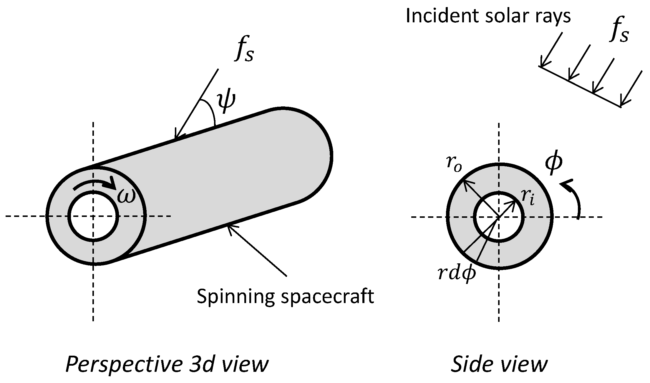
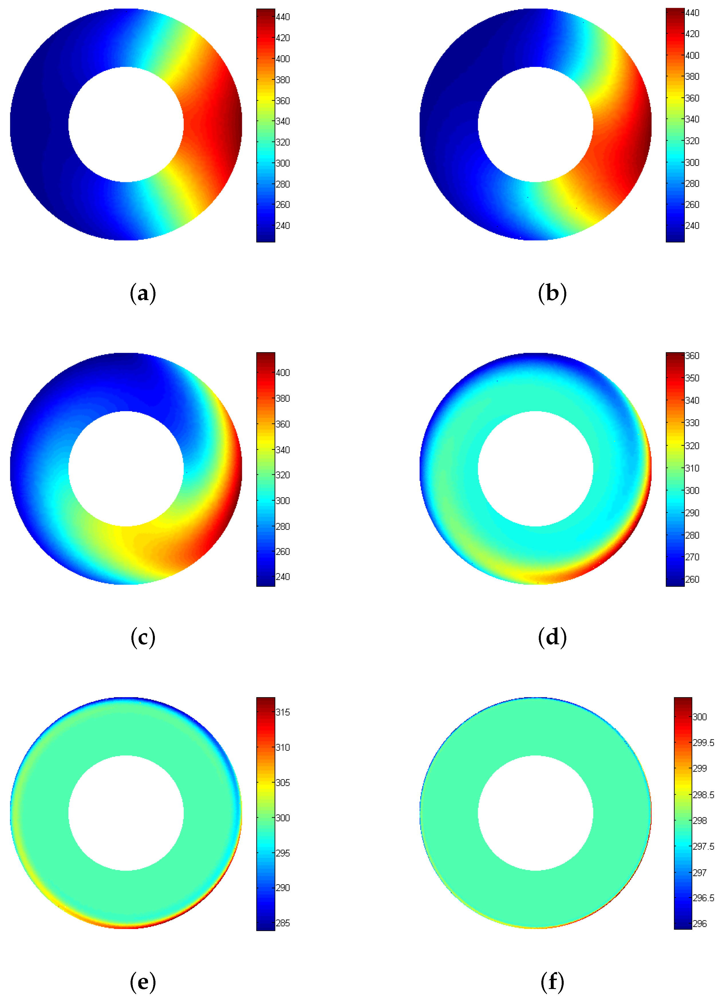
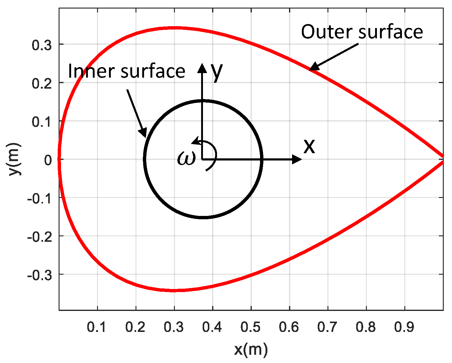
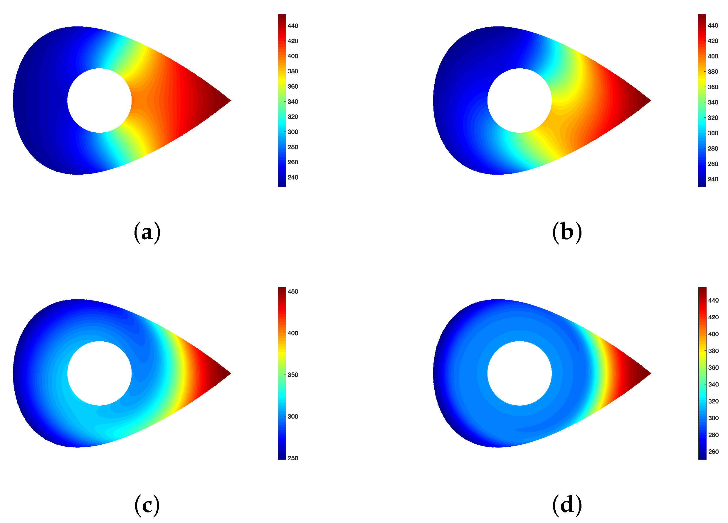
2. Heat Transfer Modeling of a Rotating Spacecraft Under Solar Radiation

The performance requirements of a spacecraft’s mission could be assessed at the earliest stages of design through the development of mathematical models and deployment of computational tools. Recent advances in computer hardware and software have enabled to reduce the computational burden associated with the numerical integration of the high-fidelity equations governing the heat transfer of the aforementioned systems [2,9,26]. Software tools can be deployed to assist the design process and provide guidelines to enable enhanced operability of spacecraft.

As a first step towards developing a good understanding of the thermal behavior of a space vehicle, being in exposure to different heat sources while traveling along the atmospheric layers, we represent this system by an infinitely long and hollow cylindrical shape rotating at constant angular speed $\omega$. The space vehicle is expected to operate in low Earth orbit environment. The inner boundary of the cylindrical vehicle is assumed fully-insulated and the outer surface is subjected to the solar radiation and the radiative heat dissipation into the surroundings. The axis of the vehicle is placed at an angle $\psi$ to the direction of the parallel rays of the impinging radiation of intensity $f_s$ as shown in Figure 1. The objective is to examine the temperature variations within the space vehicle under different operating conditions, including the spinning speed and the altitude.

The governing equation of the temperature field is given by as follows:

$$\begin{array}{c}\hfill \frac{1}{\kappa }\frac{\partial T}{\partial t}=\frac{{\partial }^{2}T}{\partial r^2}+\frac{1}{r}\frac{\partial T}{\partial r}+\frac{1}{r^2}\frac{{\partial }^{2}T}{\partial {\theta }^2}\end{array}$$

(1)

where $\kappa$ is the thermal diffusivity, T is the temperature, r is the radius coordinate, t is the time, and $\theta$ is the angular coordinate fixed in the space vehicle. Following [9], we introduce the angular coordinate as

$$\begin{array}{c}\hfill \varphi =\theta -\omega t\end{array}$$

(2)

and rewrite the governing equation as

$$\begin{array}{c}\hfill \frac{{\partial }^{2}T}{\partial r^2}+\frac{\omega }{r}\frac{\partial T}{\partial r}+\frac{\omega }{\kappa }\frac{\partial T}{\partial \varphi }+\frac{1}{r^2}\frac{{\partial }^{2}T}{\partial {\varphi }^2}=0\end{array}$$

(3)

Accounting for the effect of the solar ray incidence and the radiative heat dissipation, the boundary condition at the outer vehicle surface ($r=r_o$) can be expressed as

$$\begin{array}{c}\hfill K\frac{\partial T}{\partial r}(r_o,\varphi )=\alpha f_s\sin \left(\psi \right)g_s-\sigma ϵT^4(r_o,\varphi )\end{array}$$

(4)

where K is the thermal conductivity, $\alpha$ is the absorptivity of the surface exposed to radiation, $f_s$ is the intensity of the solar radiation, $\psi$ is the inclination the vehicle axis to the radiation axis, $\sigma$ is the Stefan-Boltzman constant, $ϵ$ is the emissivity of the vehicle surface, and $g_s$ is given by

$$g_s=\{\begin{array}{cc}\cos \left(\varphi \right),\hfill & -\frac{\pi }{2}\le \varphi \le \frac{\pi }{2}\hfill \\ 0,\hfill & \frac{\pi }{2}<\varphi <\frac{3\pi }{2}\hfill \end{array}$$

(5)

The inner vehicle surface ($r=r_i$) is insulated and the corresponding boundary condition is expressed as

$$\begin{array}{c}\hfill K\frac{\partial T}{\partial r}(r_i,\varphi )=0\end{array}$$

(6)

Expanding the nonlinear term of the outer boundary condition while assuming small temperature variation with respect to a characteristic temperature $T_o$, introducing the following dimensionless parameters [9]

$$\begin{array}{c}\hfill \widehat{T}=\frac{T}{T_o}-\frac{3}{4},\xi =\frac{r}{r_0},\beta =\sqrt{\frac{\omega }{\kappa }}{r}_0\end{array}$$

(7)

we obtain the following dimensionless governing equations and boundary conditions

$$\begin{array}{c}\hfill \frac{{\partial }^2\widehat{T}}{\partial {\xi }^2}+\frac{1}{\xi }\frac{\partial \widehat{T}}{\partial \xi }+{\beta }^2\frac{\partial \widehat{T}}{\partial \varphi }+\frac{1}{{\xi }^2}\frac{{\partial }^2\widehat{T}}{\partial {\varphi }^2}=0\end{array}$$

(8)

$$\begin{array}{c}\hfill \frac{\partial \widehat{T}}{\partial \xi }(1,\varphi )=\frac{\alpha f_s\sin \left(\psi \right)}{K{T}_o}{g}_s-\frac{4r_o\sigma ϵ}{K}{T}_o^3\widehat{T}(1,\varphi )\end{array}$$

(9)

$$\begin{array}{c}\hfill \frac{\partial \widehat{T}}{\partial \xi }({\xi }_i,\varphi )=0,{\xi }_i=\frac{r_i}{r_o}\end{array}$$

(10)

We note that the characteristic temperature $T_o$ is given by the following expression as derived in [7]

$$\begin{array}{c}\hfill T_o={\left(\frac{\alpha f_s\sin \left(\psi \right)}{\sigma ϵ\pi }\right)}^{\frac{1}{4}}\end{array}$$

(11)

The mathematical model presented above will be used to investigate the temperature distribution over a thick-walled cylindrical space vehicle rotating at different angular speeds while exposed to solar radiation.

3. Numerical Procedure: Meshless Method

3.1. Theoretical Background

Meshless methods (MMs) have been recently used to solve problems arising in physics and engineering. The motivation behind meshless methods lies in relieving the burden of mesh generation. All traditional mesh-based numerical methods have difficulties on obtaining a suitable mesh. In fact, the problem of generating meshes has become more acute in recent years. Since the application of computational methods to real world problems appears to be paced by mesh generation, alleviating this bottleneck potentially impacts an enormous field of problems.

Meshless methods are based on approximating the unknown field functions and their derivatives, by using a set of nodes, “sprinkled” over the spatial domain and, functions with compact support. Meshless schemes bypass the use of a conventional mesh. The major fields of computational mechanics, such as finite element methods (FEM), finite difference methods (FDM), and finite volume methods (FVM), rely on the use of elements, interlaced grids, or finite volumes as the underlying structures upon which to discretize governing partial differential equations (PDE). On the other hand, meshless schemes only require clouds of points, without any prior knowledge on their connectivity. On this set of nodes, the spatial domain is represented and PDEs are discretized. Local clouds for each point in a domain are proximity-based subsets of the global set of points. Local clouds of points replace the more traditional forms of connectivity found in FEM, FDM, and FVM. Several formulations of the meshfree method have been formulated such as smoothed particle hydrodynamics (SPH) [31], the diffuse approximation method (DAM) [32], and the element free Galerkin method (EFG). The present study employs the discretization corrected particle strength exchange (DC PSE) [33,34]. DC PSE was formulated as an extension of the particle strength exchange (PSE) method [35]. The latter is used for the evaluation of spatial derivatives of a continuous function, discretized over scattered collocation points. A drawback from the construction procedure of the PSE operators is the introduction of an overlap condition [36], which results in a large number of particles for small kernel sizes. For the DC PSE method, the overlap condition can be relaxed by directly satisfying discrete moment conditions over collocation points. The DC PSE operators ensure that the discretization error at the collocation points does not dominate the overall order of accuracy of the approximation. Next, we introduce the DC PSE operators for strong form formulations (excluding collocation point volumes) in 2D and how to construct them. For higher dimensions and more general analysis and discussion the reader is directed to [36].

We consider the differential operator for a continuous field function $f\left(\mathbf{x}\right)=f(x,y)$ at point ${\mathbf{x}}_i=(x_i,y_i)$

$$\begin{array}{c}\hfill {\mathbf{D}}^{(m,n)}f\left({\mathbf{x}}_i\right)=\frac{{\partial }^{m+n}}{\partial x^m\partial y^n}f(x,y){|}_{x_i,y_i}\end{array}$$

(12)

where m and n are integers that determine the order of the differential operator. We define the DC PSE operator for the spatial derivative ${\mathbf{D}}^{(m,n)}f\left({\mathbf{x}}_i\right)$ as follows:

$$\begin{array}{c}\hfill {\mathbf{Q}}^{(m,n)}f\left({\mathbf{x}}_i\right)=\frac{1}{ϵ{\left({\mathbf{x}}_i\right)}^{m+n}}\sum _{{\mathbf{x}}_j\in N\left({\mathbf{x}}_j\right)}\left(f({\mathbf{x}}_j\pm f\left({\mathbf{x}}_i\right))\right)\frac{1}{ϵ{\left({\mathbf{x}}_i\right)}^2}\eta \left(\frac{{\mathbf{x}}_i-{\mathbf{x}}_j}{ϵ\left({\mathbf{x}}_i\right)}\right)\end{array}$$

(13)

where $ϵ\left(\mathbf{x}\right)$ is a local scaling parameter, $\eta (\mathbf{x},ϵ(\mathbf{x}\left)\right)$ is a kernel function normalized by the factor $\frac{1}{ϵ{\left(\mathbf{x}\right)}^2}$, and $N\left(\mathbf{x}\right)$ is the set of points in the collocation grid within the support of the kernel function. The objective is to construct our DC PSE operators so that as the average spacing between neighbours is decreases, $h\left({\mathbf{x}}_p\right)$ tends to zero, around the point ${\mathbf{x}}_p$ and then the operator converges to the spatial derivative ${\mathbf{D}}^{(m,n)}f\left({\mathbf{x}}_i\right)$ with an asymptotic rate r, as expressed below

$$\begin{array}{c}\hfill {\mathbf{Q}}^{(m,n)}f\left({\mathbf{x}}_i\right)={\mathbf{D}}^{(m,n)}f\left({\mathbf{x}}_i\right)+O\left(h\left({\mathbf{x}}_i\right)\right)\end{array}$$

(14)

where the average neighbour spacing h is defined as

$$\begin{array}{c}\hfill h\left({\mathbf{x}}_i\right)=\frac{1}{N}\sum _{{\mathbf{x}}_i\in N\left(\mathbf{x}\right)}|x-x_i|+|y-y_i|\end{array}$$

(15)

where N is the number of points in the support domain of ${\mathbf{x}}_i$. Additionally, we define a kernel function, $\eta \left(\mathbf{x}\right)$ and a scaling relation $ϵ\left({\mathbf{x}}_p\right)$ which satisfy Equation (14). To achieve this, we begin by replacing the terms $f\left({\mathbf{x}}_i\right)$ in Equation (13) with their Taylor series expansions around the point ${\mathbf{x}}_i$. This gives

$$\begin{array}{ccc}\hfill {\mathbf{Q}}^{(m,n)}f\left({\mathbf{x}}_i\right)& =& \left(\sum _j^{\infty }\sum _k^{\infty }\frac{ϵ{\left({\mathbf{x}}_i\right)}^{j+k-m-n}{(-1)}^{j+k}}{j!k!}{\mathbf{D}}^{(j,k)}f\left({\mathbf{x}}_i\right)Z^{j,k}\left({\mathbf{x}}_i\right)\right)\hfill \\ & \pm & Z^{0,0}\left({\mathbf{x}}_i\right)ϵ{\left({\mathbf{x}}_i\right)}^{-m-n}f\left({\mathbf{x}}_i\right)\hfill \end{array}$$

(16)

where

$$\begin{array}{c}\hfill Z^{j,k}\left({\mathbf{x}}_i\right)=\sum _{{\mathbf{x}}_i\in N\left({\mathbf{x}}_q\right)}\frac{{(x_i-x_q)}^j{(y_i-y_q)}^k{(-1)}^{j+k}}{ϵ{\left({\mathbf{x}}_i\right)}^2}\eta \left(\frac{{\mathbf{x}}_i-{\mathbf{x}}_j}{ϵ\left({\mathbf{x}}_i\right)}\right)\end{array}$$

(17)

are the discrete moments. The convergence behavior of Equation (16) is determined by the coefficients of the terms $ϵ{\left({\mathbf{x}}_i\right)}^{j+k-m-n}{\mathbf{D}}^{(j,k)}$. We enforce the DC PSE operator to satisfy Equation (16) by setting the coefficients m and n of the term ${\mathbf{D}}^{(m,n)}$ equal to one, and all other coefficients equal to zero. Finally, using the kernel function we obtain

$$\begin{array}{c}\hfill {\mathbf{Q}}^{(m,n)}f({\mathbf{x}}_i=\frac{1}{ϵ{\left({\mathbf{x}}_i\right)}^{m+n}}\sum _{j\in N\left(j\right)}\left(f\left({\mathbf{x}}_j\right)\pm f\left({\mathbf{x}}_i\right)\right)p\left(\frac{{\mathbf{x}}_i-{\mathbf{x}}_j}{ϵ\left({\mathbf{x}}_i\right)}\right){\alpha }^T\left({\mathbf{x}}_i\right)e^{\frac{-{(x_i-x_j)}^2-{(y_i-y_j)}^2}{ϵ\left({\mathbf{x}}_i\right)}}\end{array}$$

(18)

The row vector $p\left(\mathbf{x}\right)$ contains monomials and vector ${\alpha }^T$ is the column vector of unknown coefficients. For example, if we set $r=2$ and approximate the first spatial derivative in the x direction ($D^{1,0}$), we have $l=6$ and the monomial basis is $p\left(x\right)=\{1,x,y,x^2,xy,y^2\}$. The discrete moment conditions can be expressed as

$$\begin{array}{c}\hfill \mathbf{A}\left(\mathbf{x}\right){\alpha }^T\left(\mathbf{x}\right)={\mathbf{b}}^T\end{array}$$

(19)

with

$$\begin{array}{c}\hfill \mathbf{A}\left(\mathbf{x}\right)={\mathbf{B}}^T\left(\mathbf{x}\right)\mathbf{B}\left(\mathbf{x}\right)\end{array}$$

(20)

$$\begin{array}{c}\hfill \mathbf{B}\left(\mathbf{x}\right)=\mathbf{E}\left(\mathbf{x}\right)\mathbf{V}\left(\mathbf{x}\right)\end{array}$$

(21)

$$\begin{array}{c}\hfill \mathbf{b}={(-1)}^{m+n}{\mathbf{D}}^{(m,n)}{\mathbf{p}\left(\mathbf{x}\right)|}_{x=0}\end{array}$$

(22)

where k is the number of points in the support domain of the operator, l is the number of moment conditions to be satisfied and $\mathbf{V}\left(\mathbf{x}\right)$ is the Vandermonde matrix, computed using the set of monomials. The matrix $\mathbf{E}\left(\mathbf{x}\right)$ is a diagonal matrix determined by the kernel’s window function

$$\begin{array}{c}\hfill \mathbf{V}\left(\mathbf{x}\right)=\left(\begin{array}{cccc}{p}_1(x_1/ϵ)& p_2(x_1/ϵ)& \cdots & p_m(x_1/ϵ)\\ p_1(x_2/ϵ)& p_2(x_2/ϵ)& \cdots & p_2(x_2/ϵ)\\ ⋮& ⋮& \ddots & ⋮\\ p_1(x_k/ϵ)& p_2(x_k/ϵ)& \cdots & p_m(x_k/ϵ)\end{array}\right)\end{array}$$

(23)

$$\begin{array}{c}\hfill \mathbf{E}\left(\mathbf{x}\right)=diag\left({\{e^{-\frac{|x_i{|}^2}{2{ϵ}^2}}\}}_{i=1}^k\right)\end{array}$$

(24)

The matrix $\mathbf{A}$, often referred to as moment matrix, gives information about the spatial distribution of the nodes ${\mathbf{x}}_i$ around the centre point $\mathbf{x}$. On the other hand, b determines the approximation properties of the kernels. From the mathematical point of view, the invertibility of matrix $\mathbf{A}$ depends entirely on that of the Vandermode matrix $\mathbf{V}$.

3.2. Generation of the Point Cloud

In the context of meshless methods, generating point clouds that represent the geometry and computing spatial derivatives is a straightforward procedure. Nodes can be selected randomly or uniformly (following a uniform (Cartesian) or irregular nodal distributions) at the interior domain and on the boundary of the geometry without no prior knowledge on their connectivity. The former is easy to construct while the second requires the use of robust triangular mesh generators.

In this study, we apply an embedded Cartesian grid method to represent the complex geometry (the two cylinders). We start the procedure by setting the boundary nodes from which we will compute the average spacing $h_c$ for the Cartesian grid (Figure 2b). The Cartesian grid step size $h_c$, is defined as the average of the inner and outer boundary nodes spacing, as given by $h_{ave}=\frac{(h_{in}+h_{out})}{2}$. From the Cartesian grid, we use only the nodes located in the interior of the domain, while special care is taken for the nodes located close to the boundary nodes. These nodes, often called as degenerated nodes, are the grid nodes with distance less than $0.2h_c$, as shown in Figure 2c. The built-in MATLAB function inpolygon has been used to define the Cartesian grid nodes that are located inside the spatial domain. Degenerated nodes are removed and not included in the point cloud, since they give rise to ill-conditioned Vandremode matrices.

3.3. Explicit Solver

The diffusion–convection problem simulating the temperature variations of the space vehicle is described by Equations (1)–(10). To implement the meshless point collocation method, it is necessary to represent the spatial domain with a set of nodes, distributed over the interior domain and on the boundary. The spatial derivatives of the dependent variable (in our case temperature) are computed by the DC PSE method. As described above, the DC PSE method computes the derivatives of temperature field in a local sense, by using the neighboring nodes. Applying the Euler explicit time integration method, one can rewrite the governing equations in the Cartesian form as follows:

$$\begin{array}{c}\hfill \frac{T^{(n+1)}-T^{\left(n\right)}}{\delta t}=-u\frac{\partial T^{\left(n\right)}}{\partial x}-v\frac{\partial T^{\left(n\right)}}{\partial y}+\kappa \left(\frac{{\partial }^2{T}^{\left(n\right)}}{\partial x^2}+\frac{{\partial }^2{T}^{\left(n\right)}}{\partial y^2}\right)\end{array}$$

(25)

where $T^{(n+1)}$ and $T^{\left(n\right)}$ are the temperature values at the current and previous time steps, respectively, and $u=r\omega \cos \left(\varphi \right)$ and $v=r\omega \sin \left(\varphi \right)$ are the velocity components. We note that the time step $\delta t$ of the explicit solver should be carefully selected to guarantee stable and accurate numerical solutions.

In the present application, Neumann boundary conditions are imposed in the inner and outer surfaces of the cylinder, as given by

$$\begin{array}{c}\hfill -K\frac{\partial T}{\partial \mathbf{r}}{|}_{r=r_i}=-K(\nabla T·\mathbf{n})=-K\left(\frac{\partial T}{\partial x}{n}^x+\frac{\partial T}{\partial y}{n}^y\right)=0\end{array}$$

(26)

$$\begin{array}{c}\hfill -K\frac{\partial T}{\partial \mathbf{r}}{|}_{r=r_o}=-K(\nabla T·\mathbf{n})=-K\left(\frac{\partial T}{\partial x}{n}^x+\frac{\partial T}{\partial y}{n}^y\right)=-\alpha f_s\sin \left(\psi \right)g_s+\sigma ϵT^4\end{array}$$

(27)

where $\mathbf{n}=(n^x,n^y)$ is the unit normal vector pointing outward. We compute the values on the boundary nodes with Neumann boundary conditions based on values of interior nodes that belong to the support domain, as shown in Figure 3.

The temperature on the inner and outer surfaces of the cylinder are computed using the Neumann boundary conditions as follows. First, we compute the weights, $w^x$ and $w^y$, for the first spatial derivative with respect to $x-$ and $y-$, respectively, based on the support nodes. The support nodes (stencil) include one boundary point (center number i) such as the stencil shown in Figure 3 and the nodes located in the interior of the geometry. The boundary values of the temperature are computed as

$$\begin{array}{c}\hfill T_i^{inner}=\frac{1}{(n_i^x{w}_i^x+n_i^y{w}_i^y)}\left(-n_i^x(w_2^x{T}_2+\cdots +w_n^x{T}_n)-n_i^y(w_2^y{T}_2+\cdots +w_n^y{T}_n)\right)\end{array}$$

(28)

$$\begin{array}{ccc}\hfill T_i^{outer}& =& \frac{1}{(n_i^x{w}_i^x+n_i^y{w}_i^y+\frac{4r_o\sigma ϵT_o^3}{K}+h)}(-n_i^x(w_2^x{T}_2+\cdots +w_n^x{T}_n)-n_i^y(w_2^y{T}_2+\cdots +w_n^y{T}_n)\hfill \\ & +& \frac{r_o\alpha f_s\sin \left(\psi \right)g_s}{K{T}_o})\hfill \end{array}$$

(29)

The computational model described above is implemented on Matlab. We discretize the spatial domain using successively finer uniform Cartesian embedded grids with spacing of $h=2.5\times {10}^{-3},1.25\times {10}^{-3}$ and $6.25\times {10}^{-4}$ m to ensure a grid independent solution, resulting in 34,580, 136,972 and 545,416 nodes, respectively. The results on the two finest grids are almost indistinguishable, indicating grid independence. Therefore, in our simulations we use the grid with a spacing of $h=1.25\times {10}^{-3}$ m. The time step used in the simulations is set to $dt={10}^{-3}$ s for all angular velocity values considered while the initial values for all flow variables at the interior points were set to zero. Computations were conducted using an Intel i7 quad core processor with 16 GB RAM.

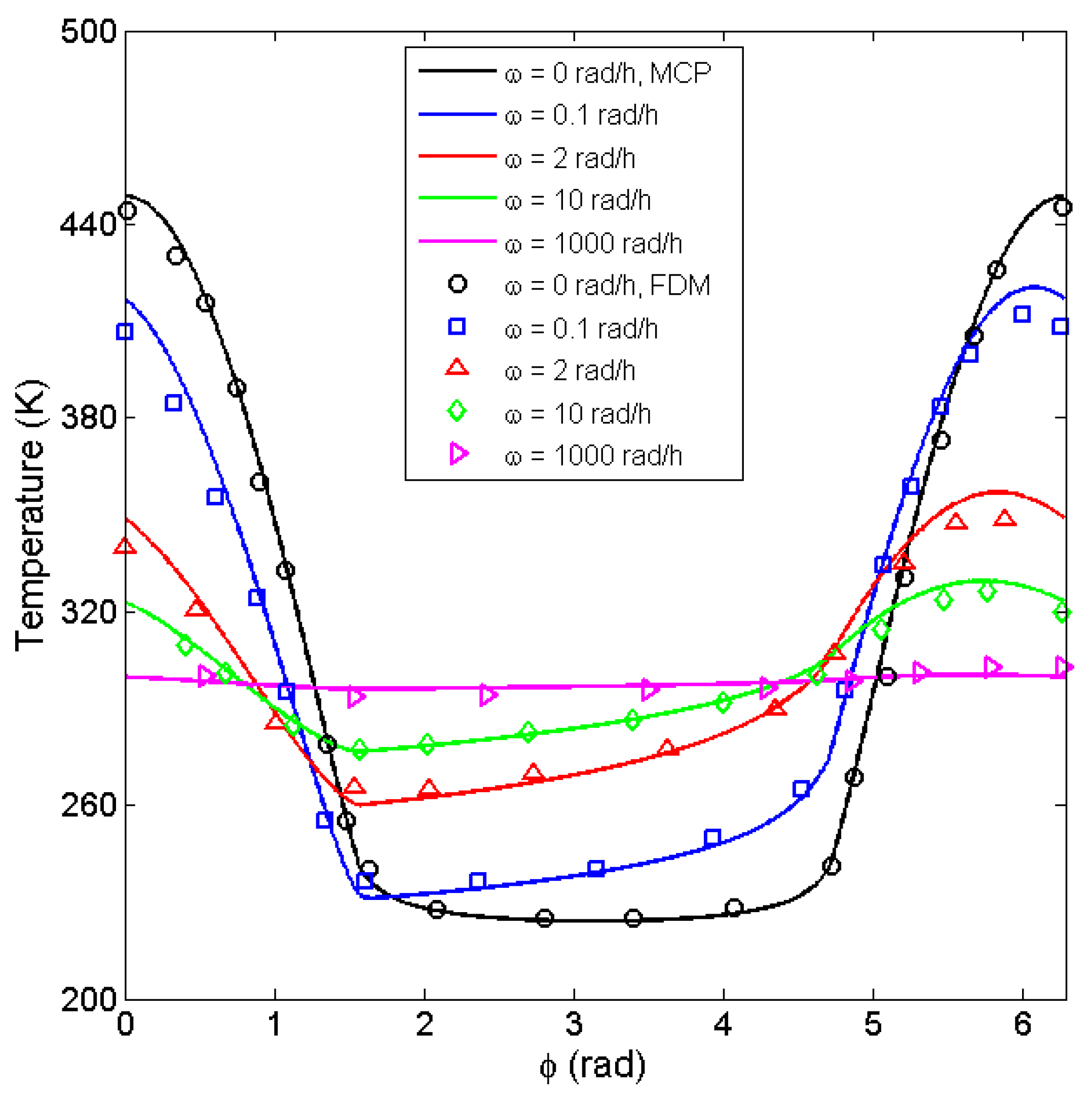
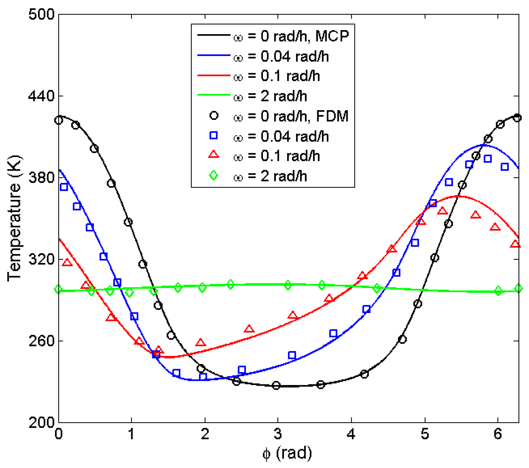
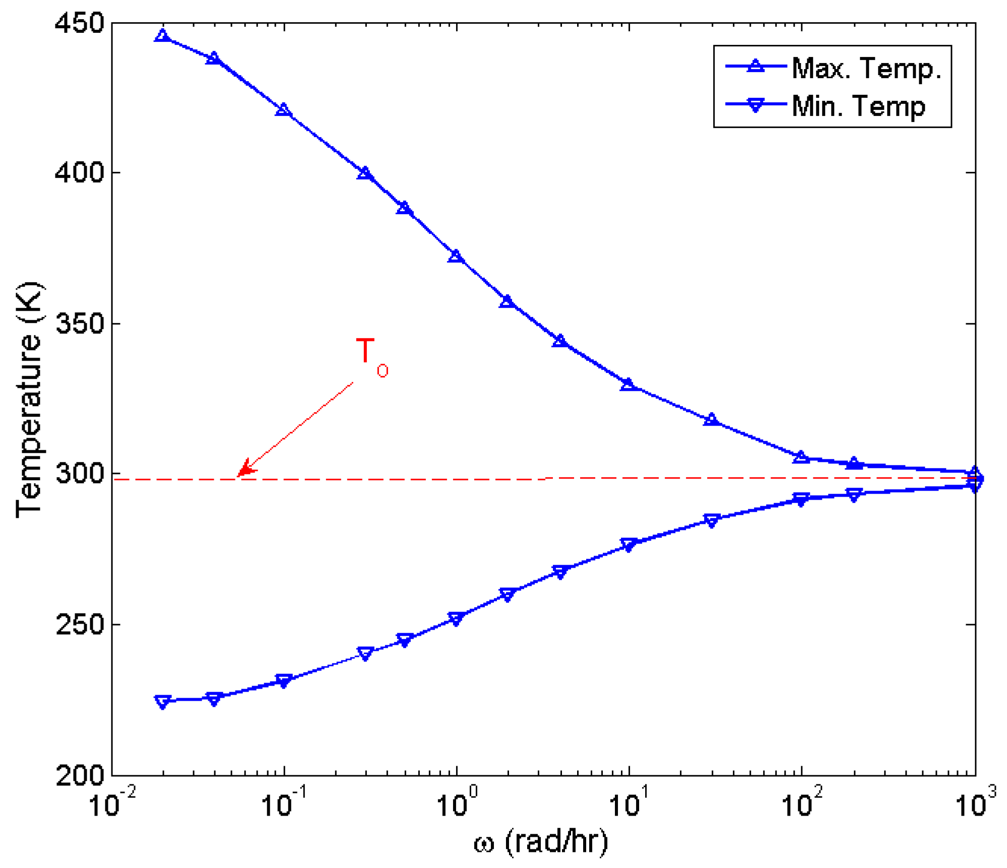
4. Results and Discussion

The developed model, given by Equations (8)–(10), is obtained by energy conservation between the heat conduction among the space vehicle, the heating from the solar radiation, the radiative heat dissipation into the surroundings while accounting for the dynamics of the space vehicle (rotational motion). This model is solved numerically using the meshless collocation point method (MCP) to evaluate the temperature distribution under different operating conditions. The simulation results are expected to provide baseline and guidance for the design of thermal control systems for space vehicles.

To verify the numerical predictions of the meshless collocation point method, we consider the simulated case of rotating cylinder exposed to solar radiation reported in [9]. The numerical values of the geometry and thermal parameters are presented in

Table 1. Numerical values of the parameters used for the rotating spacecraft [9].

Parameter	Symbol	Numerical Value
Outer radius	$r_o$	0.3048 m
Inner radius	$r_i$	0.1524 m
Inclination of the vehicle	$\psi$	$\frac{\pi }{2}$
Intensity of the sloar radiation	$f_s$	1.4 kW/m2
Thermal conductivity	K	0.173 W/m K
Absorptivity	$\alpha$	1
Emissivity	$ϵ$	1
Characteristic temperature	$T_o$	297.46 K
Non-dimensional radius	$\xi$	0.8 and 1
Spinning speed	$\omega$	0–1000 rad/h

. The vehicle is assumed to be a black body made of natural rubber with a low conductivity. We simulate the thermal response of the space vehicle while varying the spinning speed $\omega$ from 0 to 1000 rad/h. The current simulation results are compared against those obtained from the finite difference method (FDM) by Gadalla and Wehba [9]. We plot in Figure 4 the variations of the steady-state temperature at the outer surface for different spinning speeds as obtained from the two numerical approaches: MCP (current study) and FDM (as used in [9]). The two sets of data show good agreement. This demonstrates the capability of MCP method to perform thermal analysis of moving space vehicles subjected to heat sources and dissipation. For a fixed space vehicle ($\omega$ = 0 rad/h), we observe a symmetric distribution of the temperature about the location of the radiant heat source. Once the rotational motion is initiated, this symmetry is broken. As the spinning speed increases, the maximum and minimum temperatures shift to lower and higher values, respectively. Clearly, the rotational motion of the space vehicle at higher angular speeds enables further reduction in the temperature gradients. At $\omega$ = 1000 rad/h, the temperature distribution at the outer surface is found almost insensitive to the circumferential position $\varphi$.

Figure 5 depicts the variations of the temperature with the angular position $\varphi$ at the internal circumferential surface located at $\xi =0.8$. The current simulation results compare well with those obtained using FDM [9]. The simulations show that the rotational motion tends to reduce more the temperature gradients in the internal circumferential surfaces in comparison to those achieved at the outer surface, directly exposed to the solar radiation. At $\omega$ = 2 rad/h, a slight variation in the temperature distribution is observed.

Figure 6 shows the maximum and minimum temperatures at the outer surface ($\xi =1$) for different values of the spinning speed $\omega$. Rotating the space vehicle at higher speeds results in shrinking the bandwidth between the temperature extrema. At very high rotational speeds ($\omega \ge 1000$ rad/h), the maximum and minimum temperatures converge to the reference temperature $T_o$, given by Equation (11).

To gain an insight into the impact of the rotational motion on the temperature distribution over the full space vehicle, we plot in Figure 7 the temperature contours for varying spinning speeds. Again, a symmetric temperature field is obtained for a fixed space vehicle. The rotational motion breaks the symmetry and induces reduction in the temperature range. For $\omega$ higher than 10 rad/h, the temperature is observed to be varying only within a thin layer near the outer surface, otherwise constant over the internal domain. We note that these results are consistent with those obtained in [9]. The simulation results reveal the importance of incorporating the rotational motion of the spacecraft to achieve lower temperature with a uniform distribution over the entire structure. This would enable a safer operability of the spacecraft. The Earth’s atmosphere comprises four main layers. Moving upward from ground level, these layers are named the troposphere, stratosphere, mesosphere, and thermosphere, each with its own specific traits. The exposure to different heat and pressure loads within these layers present a major cause of anomalies in many space missions. The present numerical analysis shows that the design of spacecraft can be then significantly enhanced in terms of thermal resistance to the exposure to heat sources by incorporating the rotational motion.

We discretize the spatial domain shown in Figure 8 using successively finer uniform Cartesian embedded grids with a spacing of $h=1.875\times {10}^{-3},1.25\times {10}^{-3}$ and $9.3755\times {10}^{-4}$ m to verify the convergence behavior of the numerical solution and obtain a grid independent temperature solutions. We note the aforementioned spacings lead to 114,490, 256,875 and 456,057 nodes, respectively. The results on the two finest grids are almost indistinguishable, indicating grid independence. As such, in the subsequent simulations, we use a grid with spacing of $h=1.25\times {10}^{-3}$ m. The time step is set to $dt={10}^{-6}$ s, while the initial values for all flow variables at the interior points were set to zero. Computations were conducted using an Intel i7 quad core processor with 16 GB RAM.

We show in Figure 9 the contour plots of the temperature over the thick-walled vehicle for varying angular speeds. Keeping the vehicle at static position leads to a large temperature gradients. Activating the rotational motion results in a significant reduction in temperature variations and enables more uniform temperature distribution on the body of the space vehicle.

5. Conclusions

In this work, we developed a computational model based on the meshless collocation point method to simulate the temperature distribution over a rotating spacecraft under solar radiation effect. The spacecraft is treated as a thick-walled object of different geometries. The numerical results compared well with those reported in the literature. The simulations revealed that spacecraft may undergo large temperature gradients when traveling over the Earth’s atmospheric layers or in low Earth orbit. We showed the usefulness of spinning the spacecraft to avoid large temperature variations that may degrade its performance. Rotating the spacecraft at an angular speed of or higher than 10 rad/h enables a quasi-uniform temperature distribution over its internal domain. The numerical study is expected to provide a baseline for thermal control of space vehicles.

References

1. Schonberg, W.P. Studies of hypervelocity impact phenomena as applied to the protection of spacecraft operating in the MMOD environment. Procedia Eng. 2017, 204, 4–42. [Google Scholar]
2. Deim, M.; Suderland, M.; Reiss, P.; Czupalla, M. Development and evaluation of thermal model reduction algorithms for spacecraft. Acta Astronaut. 2015, 110, 168–179. [Google Scholar] [CrossRef]
3. Labibian, A.; Alikhani, A.; Pourtakdoust, S.H. Performance of a novel heat based model for spacecraft attitude. Aerosp. Sci. Technol. 2017, 70, 317–327. [Google Scholar] [CrossRef]
4. Garmendia, I.; Anglada, E.; Vallejo, H.; Seco, M. Acurate calculation of conductive conductances in complex geometries for spacecraft thermal models. Adv. Space Res. 2016, 57, 1087–1097. [Google Scholar] [CrossRef]
5. Fernandez-Rico, G.; Perez-Grande, I.; Sanz-Andres, A.; Torralbo, I.; Woch, J. Quasi-autonomous thermal model reduction for steady-state problems in space systems. Appl. Therm. Eng. 2016, 105, 456–466. [Google Scholar] [CrossRef] [Green Version]
6. Perez-Grande, I.; Sanz-Andres, A.; Guerra, C.; Alonso, G. Analytical study of the thermal behaviour and stability of a small satellite. Appl. Therm. Eng. 2009, 29, 2567–2573. [Google Scholar] [CrossRef] [Green Version]
7. Gadalla, M.A. Prediction of temperature variation in a rotating spacecraft in space environment. Appl. Therm. Eng. 2005, 25, 2379–2397. [Google Scholar] [CrossRef]
8. Gadalla, M.A. Modeling of Thermal Analysis of Rotating Space Vehicles Subjected to Solar Radiation. In Proceedings of the 28th Intersociety Energy Conversion Engineering Conference (IECEC93), ACS, Atlanta, GA, USA, 8–13 August 1993. [Google Scholar]
9. Gadalla, M.A.; Wahba, E. Computational modeling and analysis of thermal characteristics of a rotating spacecraft subjected to solar radiation. Heat Transf.-Asian Res. 2011, 40, 655–674. [Google Scholar] [CrossRef]
10. Poncya, J.; Jubineau, F.; Angelo, F.D.; Perotto, V.; Juillet, J.J. Solar orbiter-heat shield and system technology. Acta Astronaut. 2009, 65, 1076–1088. [Google Scholar] [CrossRef]
11. Corpino, S.; Caldera, M.; Nichele, F.; Masoero, M.; Viola, N. Thermal Design and analysis of a nanosatellite in low earth orbit. Acta Astronaut. 2015, 115, 247–261. [Google Scholar] [CrossRef]
12. Farrahi, A.; Perez-Grande, I. Simplified analysis of the thermal behavior of a spinning satellite flying over sun-synchronous orbits. Appl. Therm. Eng. 2017, 125, 1146–1156. [Google Scholar] [CrossRef]
13. Ross, R.G. Estimation of thermal conduction loads for structural supports of cryogenic spacecraft assemblies. Cryogenics 2004, 44, 421–424. [Google Scholar] [CrossRef]
14. Guoliang, M.; Guiqing, J. Comprehensive analysis and estimation system on thermal environment, heat protection and thermal structure of spacecraft. Acta Astronaut. 2004, 54, 347–356. [Google Scholar] [CrossRef]
15. Teofilatto, P. Preliminary aircraft design: Lateral handling qualities. Aircr. Des. 2001, 4, 63–73. [Google Scholar] [CrossRef]
16. Shen, Z.; Li, H.; Liu, X.; Hu, G. Thermal shock induced dynamics of a spacecraft with a flexible deploying boom. Acta Astronaut. 2017, 141, 123–131. [Google Scholar] [CrossRef]
17. Meese, E.A.; Norstrud, H. Simulation of convective heat flux and heat penetration for a spacecraft at re-entry. Aerosp. Sci. Technol. 2002, 6, 185–194. [Google Scholar] [CrossRef]
18. Naumann, R.J. An analytical model for transport from quasi-steady and periodic acceleration on spacecraft. Int. J. Heat Mass Transf. 2000, 43, 2917–2930. [Google Scholar] [CrossRef]
19. Pippin, G. Space environments and induced damage mechanisms in materials. Prog. Org. Coatings 2003, 47, 424–431. [Google Scholar] [CrossRef]
20. Gaite, J.; Andres, A.S.; Grande, I.P. Nonlinear analysis of a simple model of temperature evolution in a satellite. Appl. Therm. Eng. 2009, 29, 2567–2573. [Google Scholar] [CrossRef]
21. Charnes, A.; Raynor, S. Solar heating of a rotating cylindrical space vehicle. ARS 1960, 30, 479–483. [Google Scholar] [CrossRef]
22. Wu, W.-F.; Liu, N.; Cheng, W.-L.; Liu, Y. Study on the effect of shape-stabilized phase change material on spacecraft thermal control in extreme thermal environment. Energy Convers. Manag. 2013, 69, 174–180. [Google Scholar] [CrossRef]
23. Tkachenko, S.I.; Salmin, V.V.; Tkachenko, I.S.; Kaurov, I.V.; Korovin, M.D. Verifying parameters of ground data processing for the thermal control system of small spacecraft AIST based on telemetry data obtained by Samara. Orocrdia Eng. 2017, 185, 205–211. [Google Scholar] [CrossRef]
24. Han, J.H.; Kim, C.G. Low earth orbit space environment simulation and its effects. Compos. Struct. 2006, 72, 218–226. [Google Scholar] [CrossRef]
25. Azadi, E.; Fazelzadeh, S.A.; Azadi, M. Thermally induced vibrations of smart solar panel in a low-orbit satellite. Adv. Space Res. 2017, 59, 1502–1513. [Google Scholar] [CrossRef]
26. Liu, L.; Cao, D.; Huang, H.; Shao, C.; Xu, Y. Thermal-structural analysis for an attitude maneuvering flexible spacecraft under solar radiation. Int. J. Mech. Sci. 2017, 126, 161–170. [Google Scholar] [CrossRef]
27. Nicholes, L.D. Surface Temperature Distribution on Thin-Walled Bodies Subjected to Solar Radiation in Interplanetary Space; Technical Note D-584; NASA: Washington, DC, USA, 1961.
28. Roberts, A.F. Heating of cylinders by radiation; approximate formulae for the temperature distribution. ASME 1964, 64-HT-39. [Google Scholar]
29. Jenness, J.R. Temperature in a cylindrical satellite. Acta Astronaut. 1960, 5, 241–252. [Google Scholar]
30. Torres, A.; Mishkinis, D.; Kaya, T. Mathematical modeling of a new satellite thermal architecture system connecting the east and west radiator panels and flight performance. Appl. Therm. Eng. 2014, 65, 623–632. [Google Scholar] [CrossRef]
31. Gingold, R.A.; Monaghan, J.J. Smoothed particle hydrodynamics: Theory and application to non-spherical stars. Mon. Not. R. Astron. Soc. 1977, 181, 275–389. [Google Scholar] [CrossRef]
32. Nayroles, B.; Touzot, G.; Villon, P. Generalizing the finite element method: Diffuse approximation and diffuse elements. Comput. Mech. 1992, 10, 307–318. [Google Scholar] [CrossRef]
33. Schrader, B.; Reboux, S.; Sbalzarini, I.F. Discretization correction of general integral PSE operators for particle methods. J. Comput. Phys. 2010, 229, 4159–4182. [Google Scholar] [CrossRef]
34. Bourantas, G.C.; Cheeseman, B.L.; Ramaswamy, R.; Sbalzarini, I.F. Using DC PSE operator discretization in Eulerian meshless collocation methods improves their robustness in complex geometries. Comput. Fluids 2016, 136, 285–300. [Google Scholar] [CrossRef] [Green Version]
35. Eldredge, J.D.; Leonard, A.; Colonius, T.A. A General Deterministic Treatment of Derivatives in Particle Methods. J. Comput. Phys. 2002, 180, 686–709. [Google Scholar] [CrossRef] [Green Version]
36. Bourantas, G.C.; Ghommem, M.; Kagadis, G.C.; Katsanos, K.; Loukopoulos, V.C.; Burganos, V.N.; Nikiforidis, G.C. Real-time tumor ablation simulation based on the dynamic mode decomposition method. Med. Phys. 2014, 41, 053301. [Google Scholar] [CrossRef] [Green Version]
Figure 1. Schematic showing the incident solar rays and rotating coordinate system of spacecraft: an infinitely long and hollow cylindrical shape rotating at constant angular speed ω .
Processes 07 00807 g001
Figure 2. Node distribution over the simulated domain: (a) boundary nodes, (b) full set of nodes, (c) interior and boundary nodes.
Processes 07 00807 g002
Figure 3. A boundary stencil for enforcing no flux boundary conditions. The stencil is based at the one center located on the boundary. Base center marked with a square (green) and supporting centers with a circle (red).
Processes 07 00807 g003
Figure 4. Temperature variations of outer vehicle surface for varying spinning speeds: comparison between current simulations and FDM results [9].
Processes 07 00807 g004
Figure 5. Temperature variations of the internal vehicle surface ( r r o = 0.8 ) for varying spinning speeds: comparison between current simulations and FDM results.
Processes 07 00807 g005
Figure 6. Variations of the temperature extrema (maximum and minimum) at the outer surface with the spinning speed: current simulations.
Processes 07 00807 g006
Figure 7. Temperature contours obtained for different spinning speeds: current simulations. (a) ω = 0 rad/h, (b) ω = 0.02 rad/h, (c) ω = 0.1 rad/h, (d) ω = 1 rad/h, (e) ω = 10 rad/h, (f) ω = 1000 rad/h.
Processes 07 00807 g007
Figure 8. Schematic of the cross section of the rotating space vehicle.
Processes 07 00807 g008
Figure 9. Temperature contours obtained for different spinning speeds: current simulations. (a) ω = 0 rad/h, (b) ω = 0.1 rad/h, (c) ω = 1 rad/h, (d) ω = 10 rad/h.
Processes 07 00807 g009