Numerical Study of the Unsteady Flow Characteristics of a Jet Centrifugal Pump under Multiple Conditions


1
School of Energy and Power Engineering, Lanzhou University of Technology, Lanzhou 730050, China
2
Key Laboratory of Fluid Machinery and Systems, Lanzhou 730050, China
*
Authors to whom correspondence should be addressed.
Processes 2019, 7(11), 786; https://doi.org/10.3390/pr7110786
Submission received: 28 September 2019
/
Revised: 21 October 2019
/
Accepted: 28 October 2019
/
Published: 1 November 2019
(This article belongs to the Special Issue CFD Applications in Energy Engineering Research and Simulation)
Abstract
:To study the reasons for the low efficiency of jet centrifugal pumps (JCPs) and the mechanism of unsteady flow characteristics under multiple conditions, taking a JET750G1 JCP as the object, three-dimensional steady and unsteady numerical calculations of the model pump were carried out using the k–ω turbulence model. The transient fluctuation characteristics of the flow field in the major flow passage components and the spatial and temporal evolution laws of vortices in the rotor–stator cascades were analyzed. The accuracy of the numerical method was verified by experiments. The results show that there are various scales of flow distortion phenomena in the chamber of the JCP, such as eddies, blockage of the flow passage, recirculation, secondary flow, and circulation, which not only cause great hydraulic loss, but also destroy the flow stability, symmetry, and balance in the other flow passage components. This is an important reason for the obviously lower efficiency of a JCP compared to a general centrifugal pump. The spatial and temporal evolution laws of vortices in the rotor–stator cascades are mainly related to the relative positions of the impeller blades and guide vane blades. The formation mechanism of the unsteady flow field fluctuation characteristics of JCPs is mainly related to the number of blades in the rotor–stator cascades and the operation parameters of the pump. The fluctuation intensity of the flow field inside the impeller and guide vane is obviously greater than that in the other flow areas, reflecting that the rotor–stator interaction is the decisive factor affecting the unsteady flow characteristics of a JCP under multiple conditions.
1. Introduction
The flow passage components of a jet centrifugal pump (JCP) have relatively more complex internal flow, which leads them to have shortcomings such as low efficiency, easy cavitation, and high noise. However, JCPs have been widely used in many industries and fields because of their good low-level water-lifting capacity and self-priming performance [1,2]. Compared with a general centrifugal pump, the JCP has an additional self-circulating ejector device at the impeller inlet [3]; therefore, its working principle is rather special. As a self-priming pump, the analysis, optimization, and improvement of the self-priming performance of the JCP using numerical or experimental methods has been the research focus of scholars. Wang et al. [4] performed unsteady calculations of a typical self-priming centrifugal pump and simulated the gas–fluid two-phase flow in the self-priming process. It was found that the whole self-priming process of a self-priming pump can be divided into three stages: the initial self-priming stage, the middle self-priming stage, and the final self-priming stage. Wang et al. [5] numerically studied the influence of adding anti-circulation ribs at the back of the guide vane on gas–liquid mixing and separation in the pump chamber using the Euler–Euler multiphase model. The results showed that adding ribs could reduce the gas-phase volume fraction at the inlet of the ejector and the outlet of the nozzle, improving the gas-phase volume fraction at the outlet of the pump chamber and the self-priming performance. In addition, the authors of [6] optimized the structural parameters of the jet and impeller by an orthogonal experimental method, which improved the pump efficiency by about 5% under the design conditions. Liu et al. [7,8] studied the effects of different combinations of geometric parameters such as the total length, angle, outlet length, and outlet diameter of the ejector on the gas–liquid flow of the pump and obtained the optimum combination of parameters of the ejector. They added a diversion device at the outlet of the impeller of the JCP and found that the gap between the separating flow board and impeller could not only prevent the formation of circulation of the fluid, reduce hydraulic loss, and improve the efficiency of the pump, but also quicken the mixing of the gas and liquid near the gap and shorten the self-priming time of the pump. Wang et al. [9] studied the self-priming process of a JCP by numerical and experimental methods and analyzed the gas–liquid mixing, separation, and escape, as well as the variation of the velocity, pressure, and volume fraction of gas in the pump during the self-priming process. Zhang et al. [10] experimentally studied the cavitation and energy characteristics of a JCP at different installation heights and numerically analyzed flow characteristics at 0-m heights based on the k–ω turbulence model and Zwart–Gerber–Belamri cavitation model. They reported that high-speed reflux and strong shear flow in the ejector are important reasons for the low efficiency and easy cavitation of the pump.
With the rapid development of computer technology and numerical theory, computational simulation has been widely used in the field of hydraulic machinery. Scholars have performed many studies on the steady or unsteady flow field characteristics of JCPs [11,12,13,14,15], but they have not yet given a reasonable and full account of the low efficiency and the formation mechanism of unsteady fluctuation characteristics. In this paper, a numerical method was employed to study the unsteady flow characteristics of a JET750G1 JCP under multiple conditions. The reasons for the low efficiency and the formation mechanism of the unsteady flow characteristics of the pump are analyzed with respect to the flow pattern, distribution characteristics of the time-averaged flow field and fluctuation intensity, spatial and temporal evolution process of vortices in the rotor–stator cascades, and pressure fluctuation characteristics in the major flow passage components. This provides a theoretical basis for the design and optimization of JCPs with high efficiency and low energy consumption.
2. Research Method and Model
2.1. The Model Pump
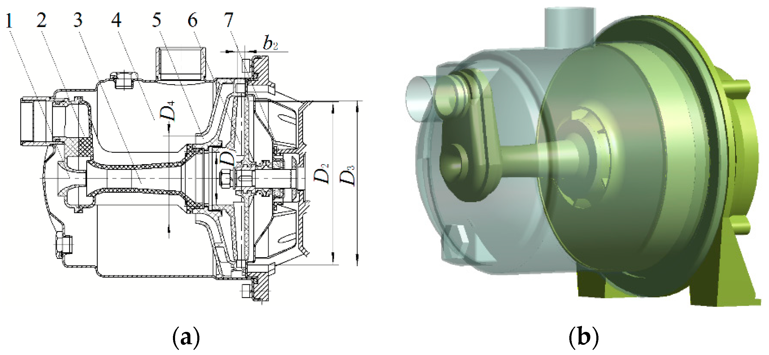
The parameters of the model JCP are as follows: rated flow Qd = 2.5 m3/h, rated water head Hd = 23 m, rated efficiency ηd = 20%, rotational speed n = 2850 r/min, shaft-passing frequency SPF = 47.5 Hz, blade-passing frequency of impeller BPFI = 285 Hz, and blade-passing frequency of guide vane BPFG = 237.5 Hz. The main geometric parameters of the impeller and guide vane are listed in Table 1. Two- and three-dimensional structure diagrams of the model pump are shown in Figure 1.
2.2. Numerical Method
The whole computational domain included the impeller, guide vane, ejector, front pump cavity, back pump cavity, inlet pipe, outlet pipe, and pump chamber. ANSYS-ICEM (16.0 ANSYS, Inc., Canonsburg, PA, USA) was employed to construct the discrete computational domain; hexahedral structured meshes were employed to form the computational domain of the impeller, guide vane, and ejector nozzle and tube, and tetrahedral unstructured meshes were employed to form the other flow passage components. The grid independence verification is shown in Table 2, which is divided into six mesh schemes according to the density of the grid. While the accuracy and efficiency of the calculation were taken into account, comparing the head prediction value of different schemes, among schemes 4, 5 and 6, increasing the amount of mesh does not have too much of an influence on the result, which means that scheme 4 has enough accuracy. Therefore, scheme 4 was chosen as the final computational mesh to conduct the simulation. The meshes of the impeller, guide vane, and jet of the model pump are shown in Figure 2.
CFX 16.0 (16.0, ANSYS Inc., Pittsburgh, PA, USA) was employed for the flow field calculations. The impeller flow fields were calculated in the rotating coordinate system in the multi-coordinate system, and the flow fields of the other components were calculated in the stationary coordinate system. The k–ω turbulence model was adopted, as the performance of this model is better than that of the k–ε model in near-wall flow analysis [16]. GGI (general grid interface) technology was employed to exchange data between the rotor and stator. Pressure inlet and velocity outlet boundary conditions were set, and the inlet pressure values were set according to the values obtained from experiments. All the solid walls were provided with non-slip wall conditions, and the roughness was set to 25 μm according to actual processing. In the steady simulation process, the interface models between rotating–stationary and stationary–stationary domains were selected as a frozen-rotor and general connection, while the governing equations were solved by a second-order upwind formula. For transient simulation, the transient rotor–stator interface model was used for the rotating–stationary interface, while the time-term was discreted by a second-order implicit scheme. The time-step size determines the precision of post-processing; therefore, the setting of the time-step requires an adequate response resolution to the flow field fluctuation. Finally, the time-step is 0.000117 s, which means that the impeller rotates about 2 degrees per time-step and 180 steps in a circle. All residuals were less than 10-5.The simulation was completed on a workstation with 20 cores and 128 GB of memory. For a model, it takes 90 min to complete 2000 steps of steady calculation, and about 1000 min to complete the transient calculation of 13 impeller cycles.
2.3. Numerical Validation
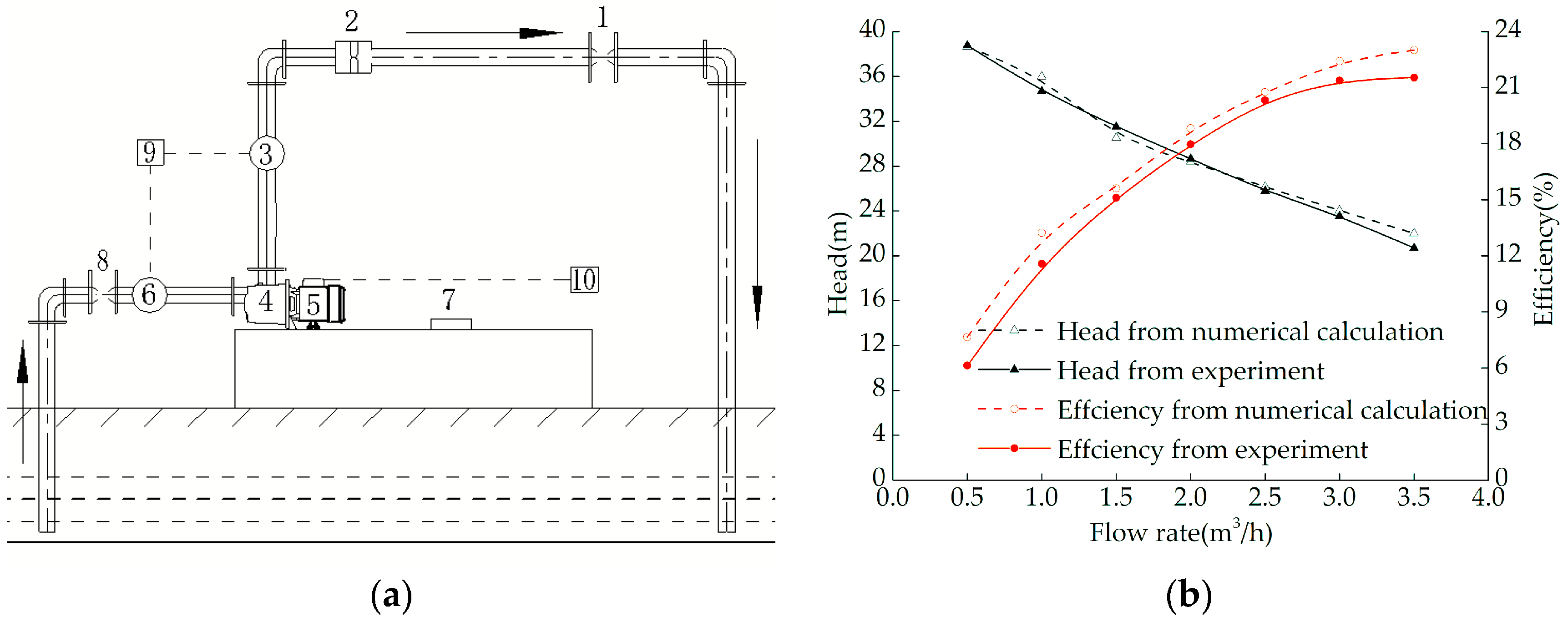
Validation of the numerical calculation of the flow fields was performed at the JCP test bed for hydraulic performance and hydrodynamic noise in the Key Laboratory of Fluid Machinery and Systems, Gansu Province. The test device consists of two parts: an operation system and a data acquisition system. The operation system meets the requirements of the operation of the pump under various conditions, including pump, circulation pipeline, motor, valves, frequency converter, and water box; the data acquisition system collects the relevant transient and steady physical quantities generated during the operation of the pump by various sensors, and then converts it into identifiable data signals through a series of processing. The related instruments include the computer, pressure sensors, flowmeter, measuring instrument of electric power, and tachometer. The flow of the pump can be changed by adjusting the inlet valve. The test system is shown in Figure 3a.
Comparison curves of the hydraulic performance between the experiment and numerical simulation are shown in Figure 3b. It can be seen that the variation trends of the performance curves are consistent between the numerical calculation and experiment, and the values at different working points are close. The maximum error in the water head was 4.6%, and that in efficiency was 4.1%, which proves the accuracy of the calculation results.
3. Analysis of the Velocity Vector and Streamline
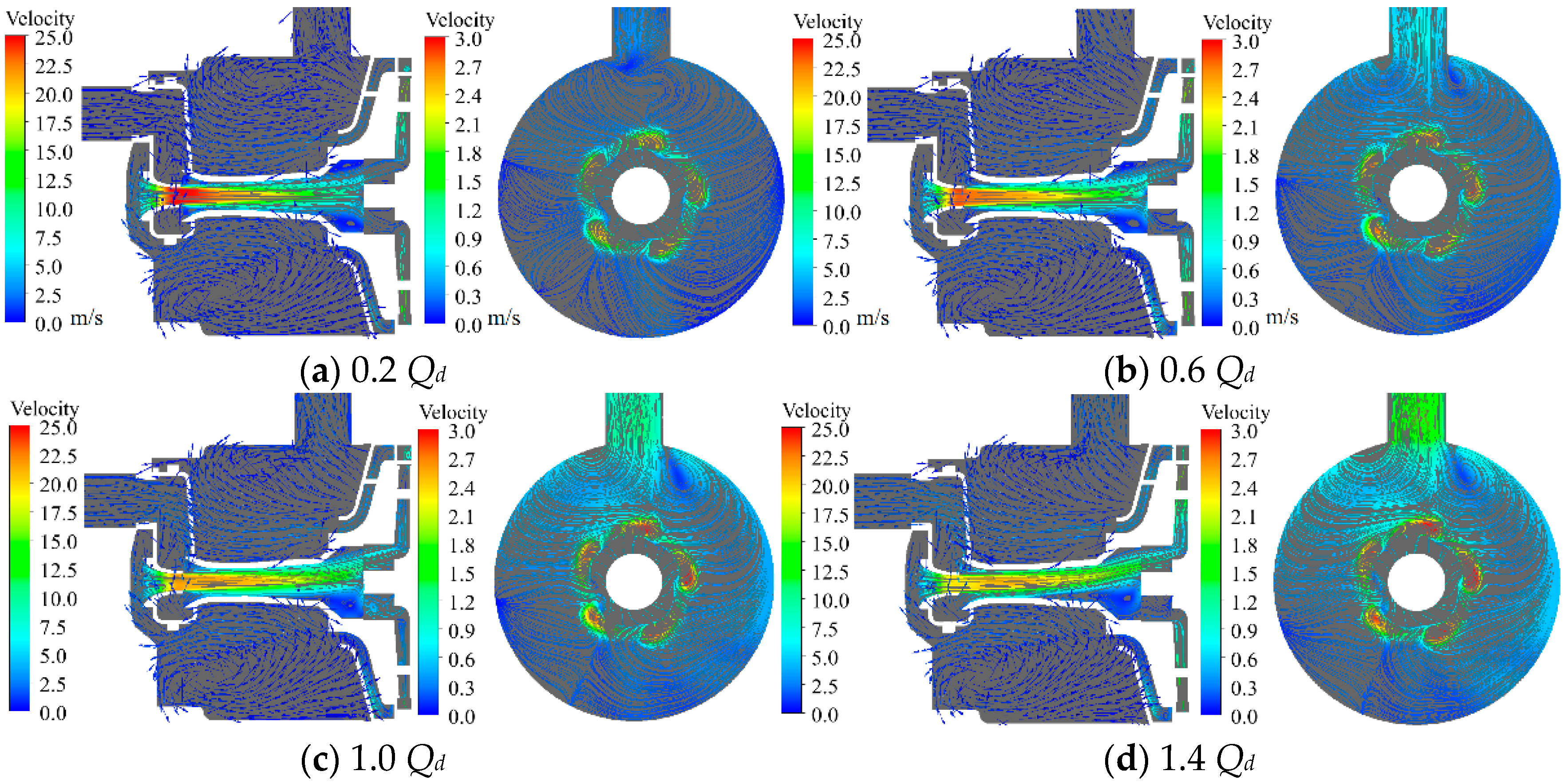
The velocity vector and streamline diagrams through the inlet and outlet tangent planes of the JCP under four conditions are shown in Figure 4; 0.2 Qd, 0.6 Qd, 1.4 Qd represent conditions at which the pump provides 20%, 60%, and 140% of the rated flow, respectively. It can be seen that there are obvious eddies in the lower half of the pump chamber near the inlet side under each condition; the flow velocity in this area is slow, and the flow passage is seriously blocked, which affects the normal flow in the upstream and downstream flow passage components and leads to obvious recirculation at the border of the impeller and ejector. Under the conditions of small flow rates, there are eddies near the outlet in the upper half of the pump chamber, and the smaller the flow rate, the more obvious the eddies. The eddies in the upper and lower sides of the pump chamber cause a blockage of the outlet channels in both sides of the ejector tube, where the flow is relatively more symmetrical. With the increasing flow rate, the eddies in the upper side of the pump chamber gradually weaken, while the eddies in the lower side gradually strengthen, and the flow in the ejector tube shows a tendency of upward deviation. There is obvious circulation movement in the pump chamber, and the flow patterns of the left and right sides are also not balanced; this is related to the asymmetry of the guide vane blades, of which there are five. There is a counter-clockwise eddy along the circumferential direction near the right-hand side of the outlet pipeline in the pump chamber, and the greater the flow rate, the greater the eddy. The area with the fastest velocity in the pump chamber is located in the circle near the ejector tube, and the flow in this area is very complicated.
The above analysis shows that there exist various sizes and scales of eddies, channel blockage, back flow, secondary flow, circulation, and other phenomena of flow field distortion in the pump chamber under multiple conditions. These not only result in great hydraulic losses but also destroy the stability, symmetry, and balance of other flow passage components, and are an important reason for the JCP’s efficiency being significantly lower than that of a general centrifugal pump.
4. Analysis of Unsteady Flow Field Characteristics Based on a Statistical Method
The unsteady flow characteristics of the model pump were analyzed by a statistical method. The unsteady physical quantities include two parts on each grid node (x, y, z) of the flow domain, the time-averaged component and the periodic component , where the periodic component represents the variation of the physical quantities in a rotation period of the impeller [17]. The two components are respectively expressed as follows:
where n, N, and t0 are grid nodes, the number of samples in an impeller rotating period, and the starting time of the rotation cycle, respectively.
The non-dimensional standard deviation of the periodic component is defined as the flow field fluctuation intensity, including the pressure fluctuation intensity, velocity fluctuation intensity, turbulence energy fluctuation intensity, etc.
The pressure fluctuation intensity is expressed as:
The velocity fluctuation intensity is expressed as:
The turbulence energy fluctuation intensity is expressed as:
where U2 means the circumferential speed at the impeller outlet.
4.1. Time-Averaged Distribution Characteristics of the Flow Field
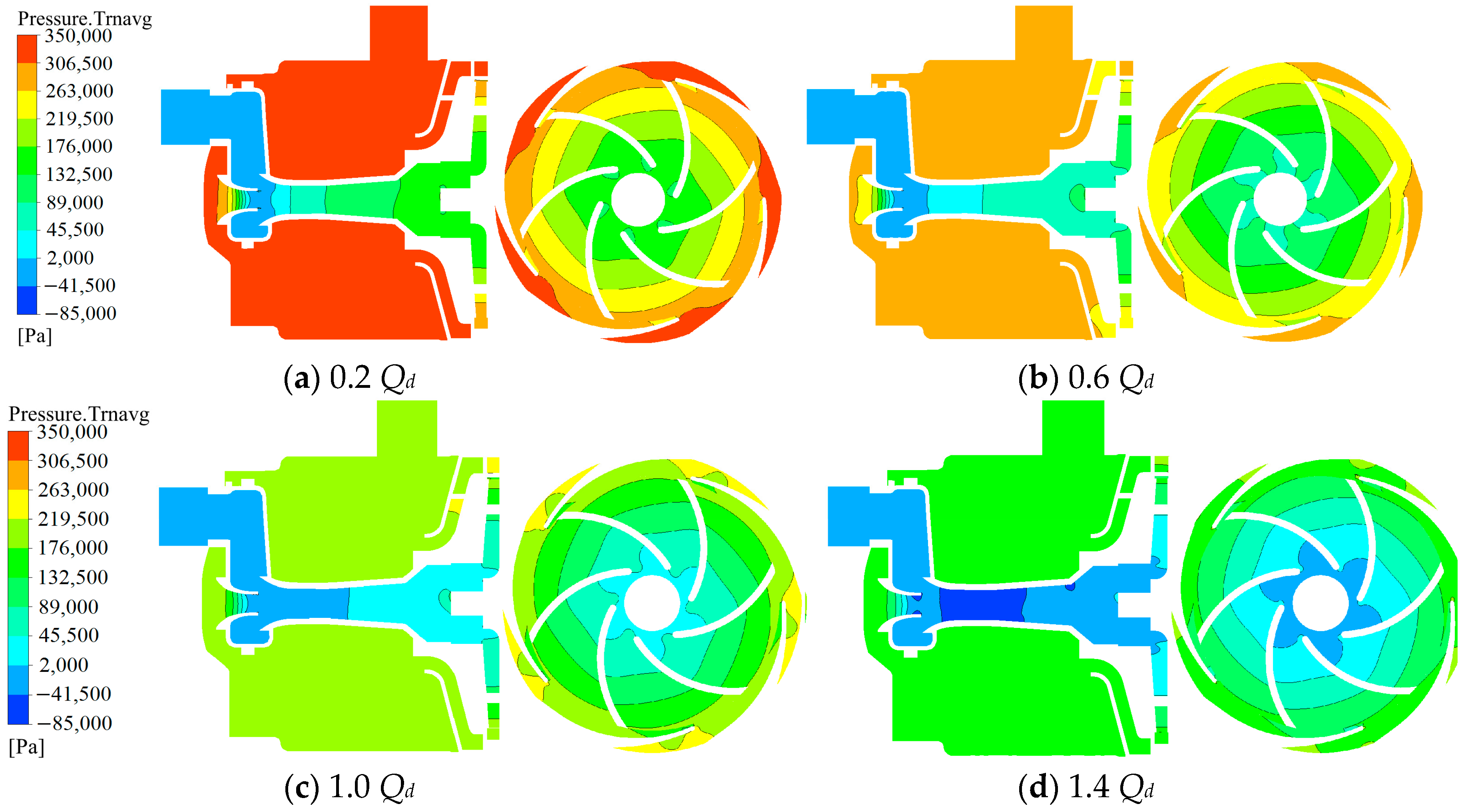
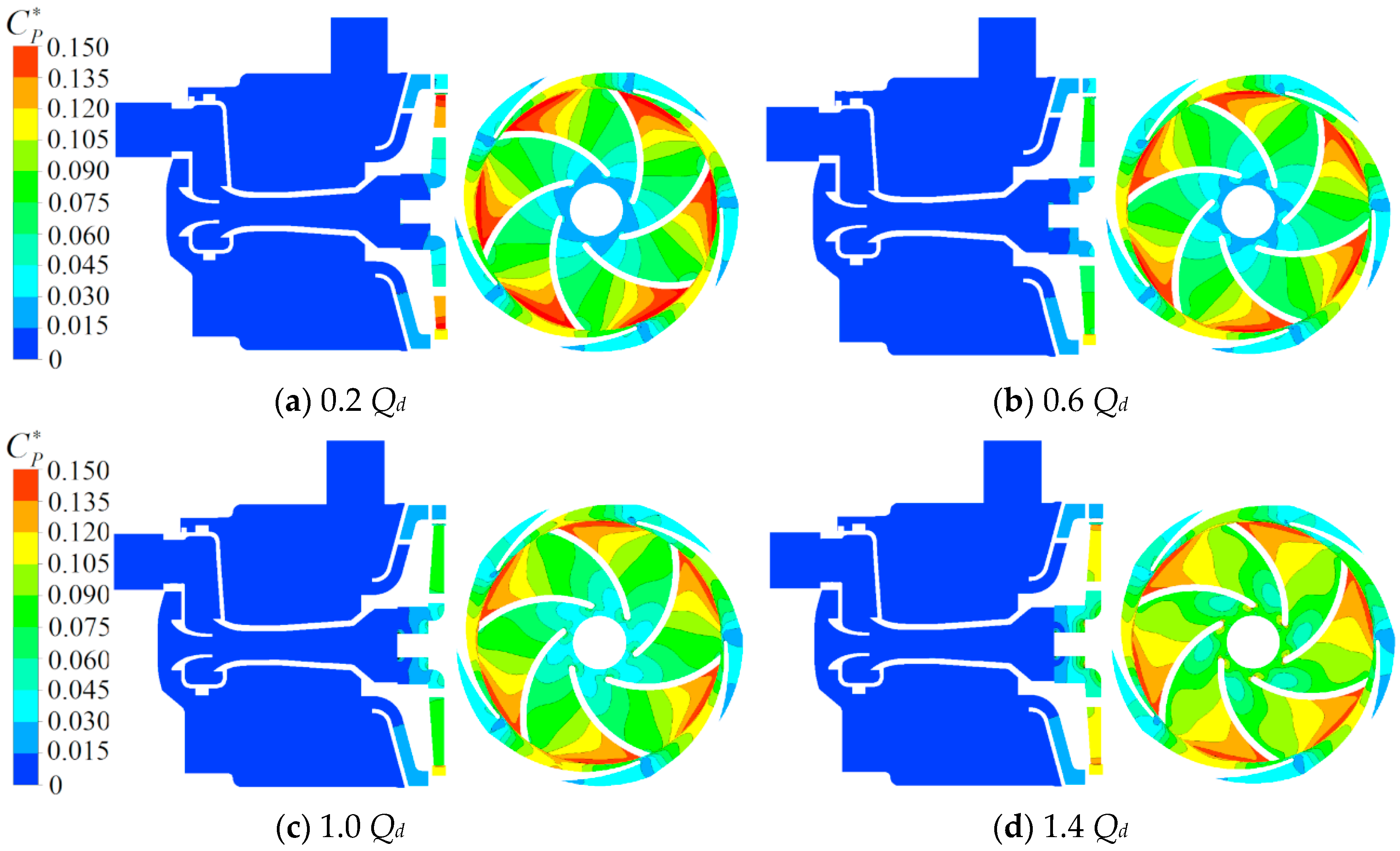
Figure 5 shows the time-averaged distribution contours of pressure on two planes under four conditions. It can be seen that the pressure in each flow passage component decreases gradually with the increasing flow rate. At small flow rates, the lowest area of pressure is located at the ejector nozzle outlet. As the flow rate increases, the lowest area gradually shifts and expands to the middle of the ejector tube, which shows that unlike the cavitation of a general centrifugal pump, which first occurs in the inlet area of the impeller, the cavitation of a JCP first occurs in the ejector.
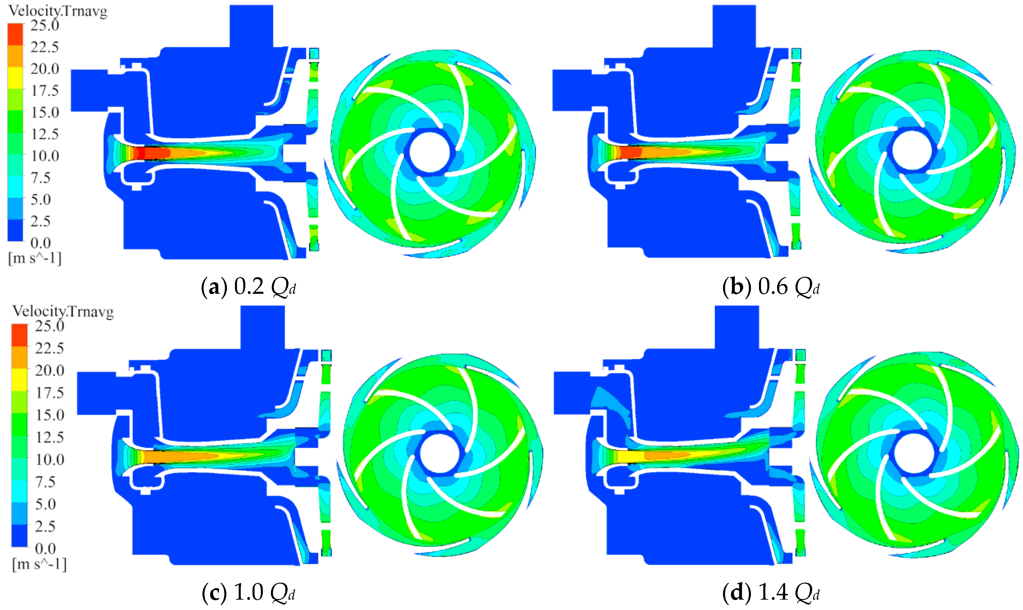
Figure 6 shows the time-averaged distribution contours of absolute velocity on two planes under four conditions. It can be seen that the difference in velocity is small in the pump chamber, guide vane, and impeller among the different working conditions, but it is large in the ejector nozzle and tube, and the largest velocity appears in the area of the nozzle exit. As the flow rate increases, the velocity in the ejector nozzle and tube decreases gradually and the distribution symmetry becomes worse and worse, showing characteristics of upward inclination. By comparing with Figure 4, we can see that this is because with the increasing flow rate, the blockage in the upper side of the ejector exit gradually weakens while it gradually increases in the lower side, and the flow then moves upward.
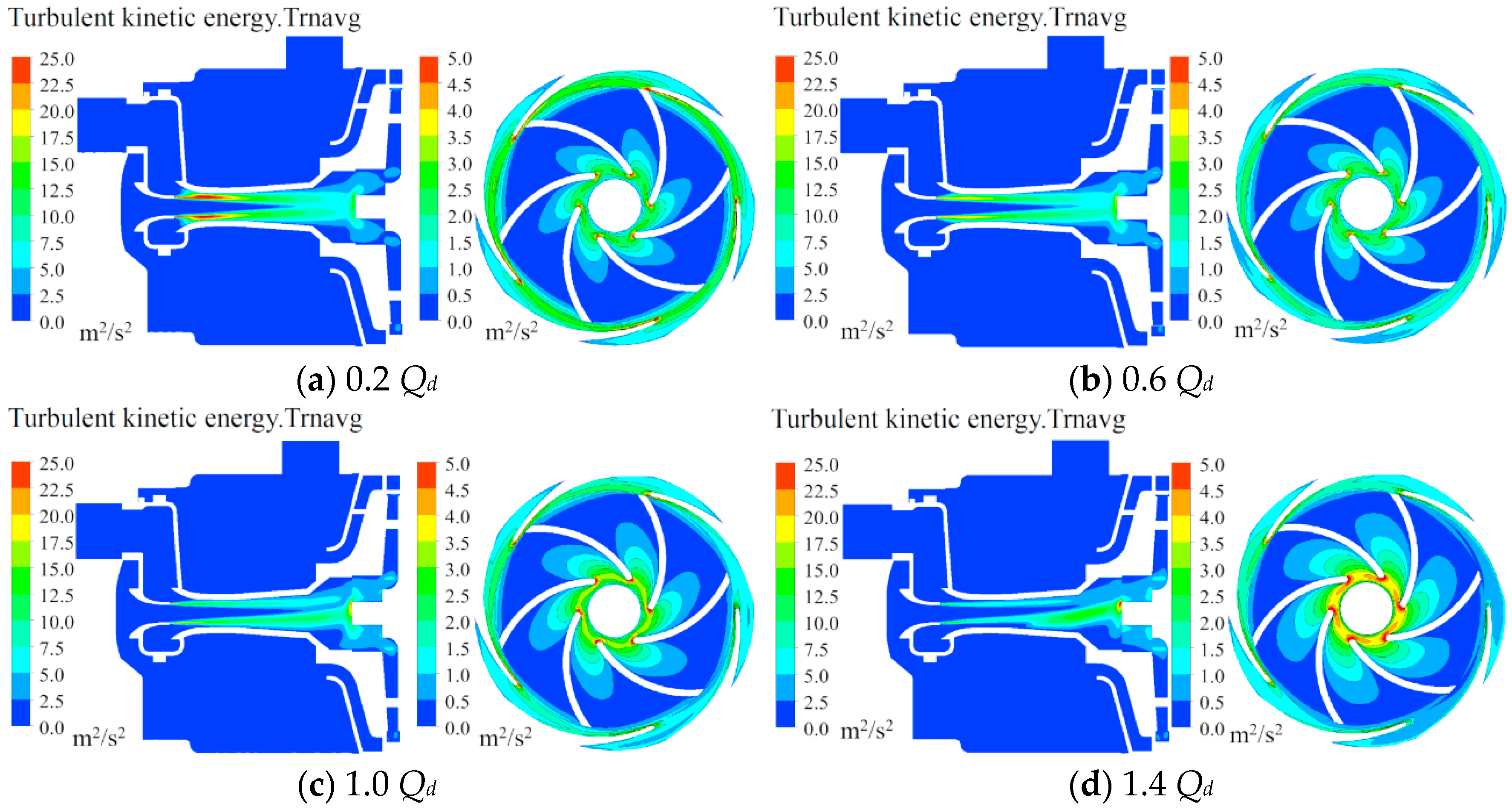
Figure 7 shows the time-averaged distributions of turbulent kinetic energy contours on two planes under four conditions. As can be seen in the figure, the turbulent kinetic energy is greater in the ejector tube and nozzle under every condition. At small flow rates, the maximum value is located around the nozzle outlet. By comparing with Figure 6, it can be seen that this is due to the mixing of high-speed flow at the nozzle outlet and low-speed flow from the pump inlet in this area, which leads to some larger vortices around the nozzle area and very violent turbulent movement. As the flow rate increases, the turbulent kinetic energy at the inlet of the impeller increases gradually, while it decreases gradually at the junction area of the rotor–stator cascades. Similar to the distribution of the velocity field, the turbulent kinetic energy field in the ejector tube shifts upward with the increasing flow rate.
4.2. Distribution Characteristics of the Fluctuation Intensity of the Flow Field
Figure 8 shows the distributions of pressure fluctuation intensity contours on two planes under four conditions. It can be seen that the pressure fluctuation intensity in the impeller and guide vane is obviously greater than that in other flow passage components, which is influenced by the rotor–stator interaction. The maximum value of the intensity appears near the pressure surface of the impeller outlet. As the flow rate increases, the fluctuation intensity decreases gradually near the junction area of the impeller and guide vane, but it increases gradually at the impeller inlet.
Figure 9 shows the distributions of velocity fluctuation intensity contours on two planes under four conditions. It can be seen that, similar to the law of the pressure fluctuation intensity distribution, the velocity fluctuation intensity in the impeller and guide vane is obviously greater than that in other flow passage components due to the rotor–stator interaction, and the maximum intensity appears in the impeller inlet area; with the increasing flow rate, the velocity fluctuation intensity increases gradually at all positions.
Figure 10 shows the distribution contours of the turbulent kinetic energy fluctuation intensity on two planes under four conditions. It can be seen that the region of the largest intensity is at the impeller inlet, which is similar to the distribution law of the velocity fluctuation intensity. As the flow rate increases, the fluctuation intensity in the impeller inlet increases gradually, while it decreases gradually in the junction area of the rotor–stator cascades.
The analysis of Figure 8, Figure 9 and Figure 10 shows that the fluctuation intensity of the flow field in the impeller and guide vane is obviously greater than that in other flow passage areas, reflecting that the rotor–stator interaction plays a decisive role in the unsteady fluctuation intensity of the flow field of a JCP.
5. Analysis of Spatial–Temporal Evolution of Vortices in the Rotor–Stator Cascades
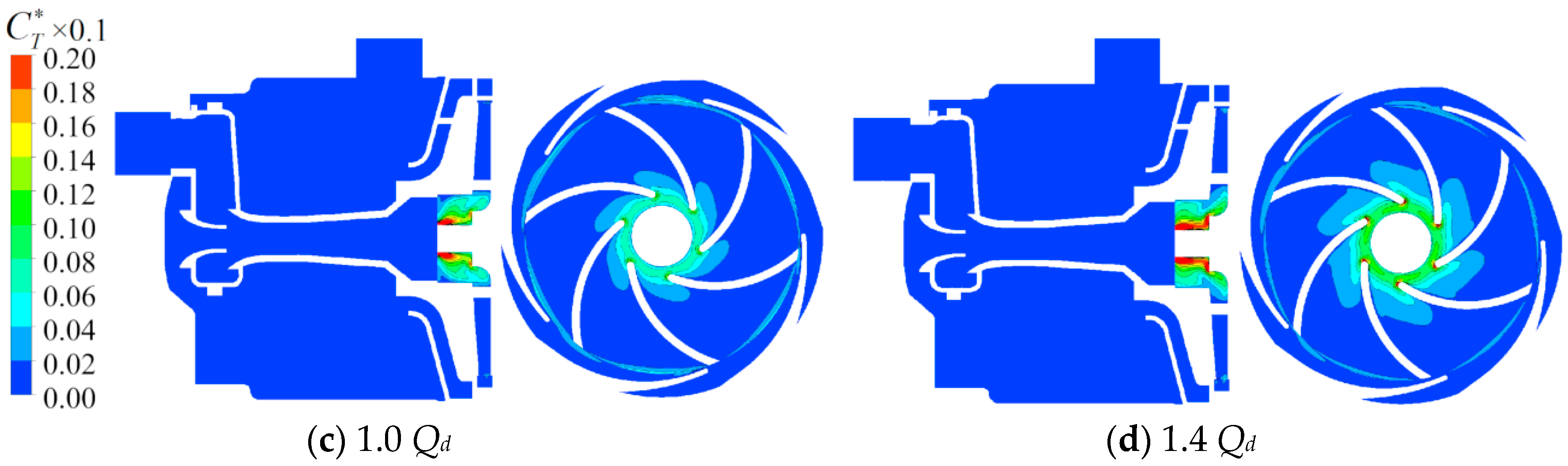
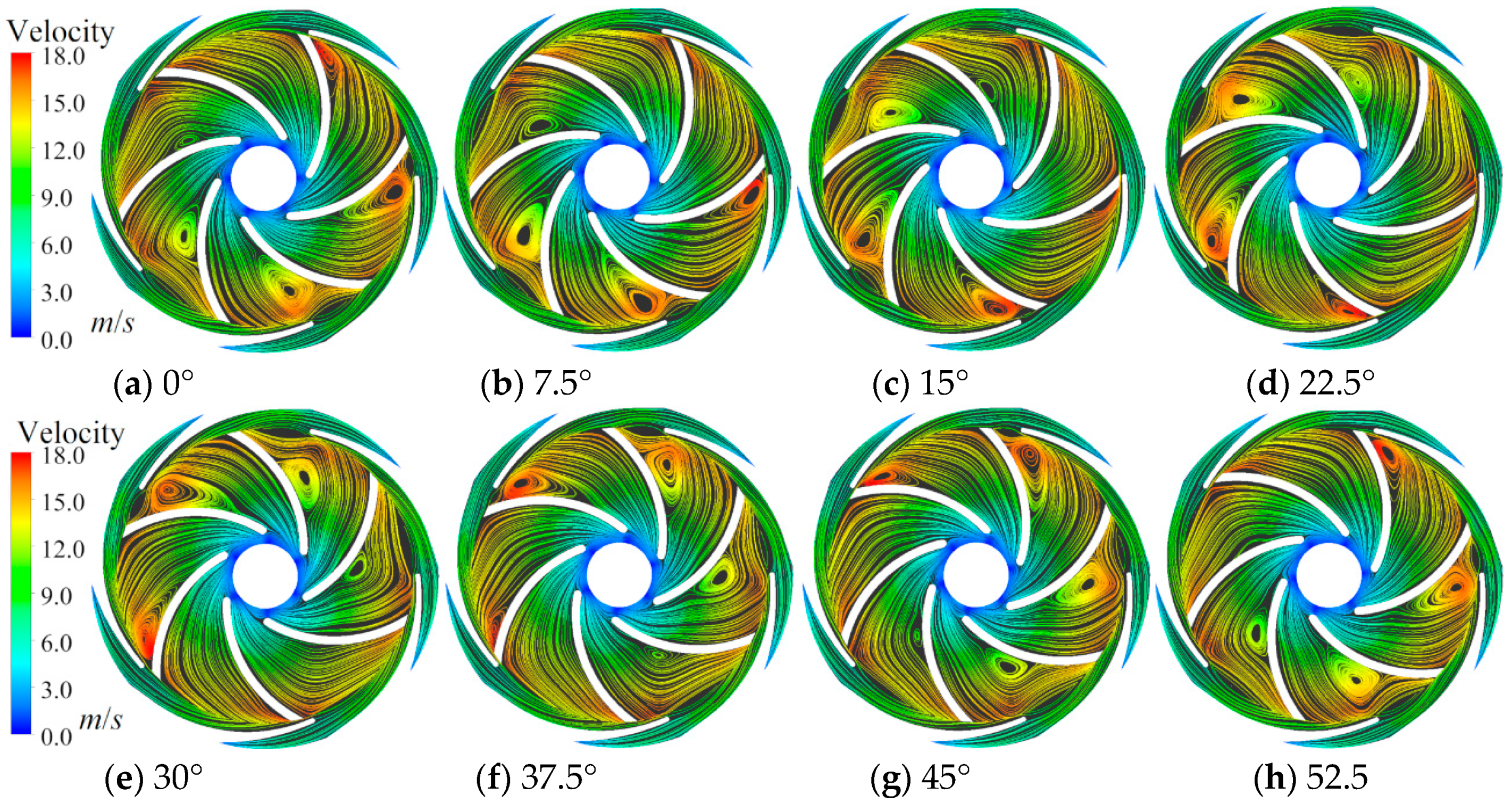
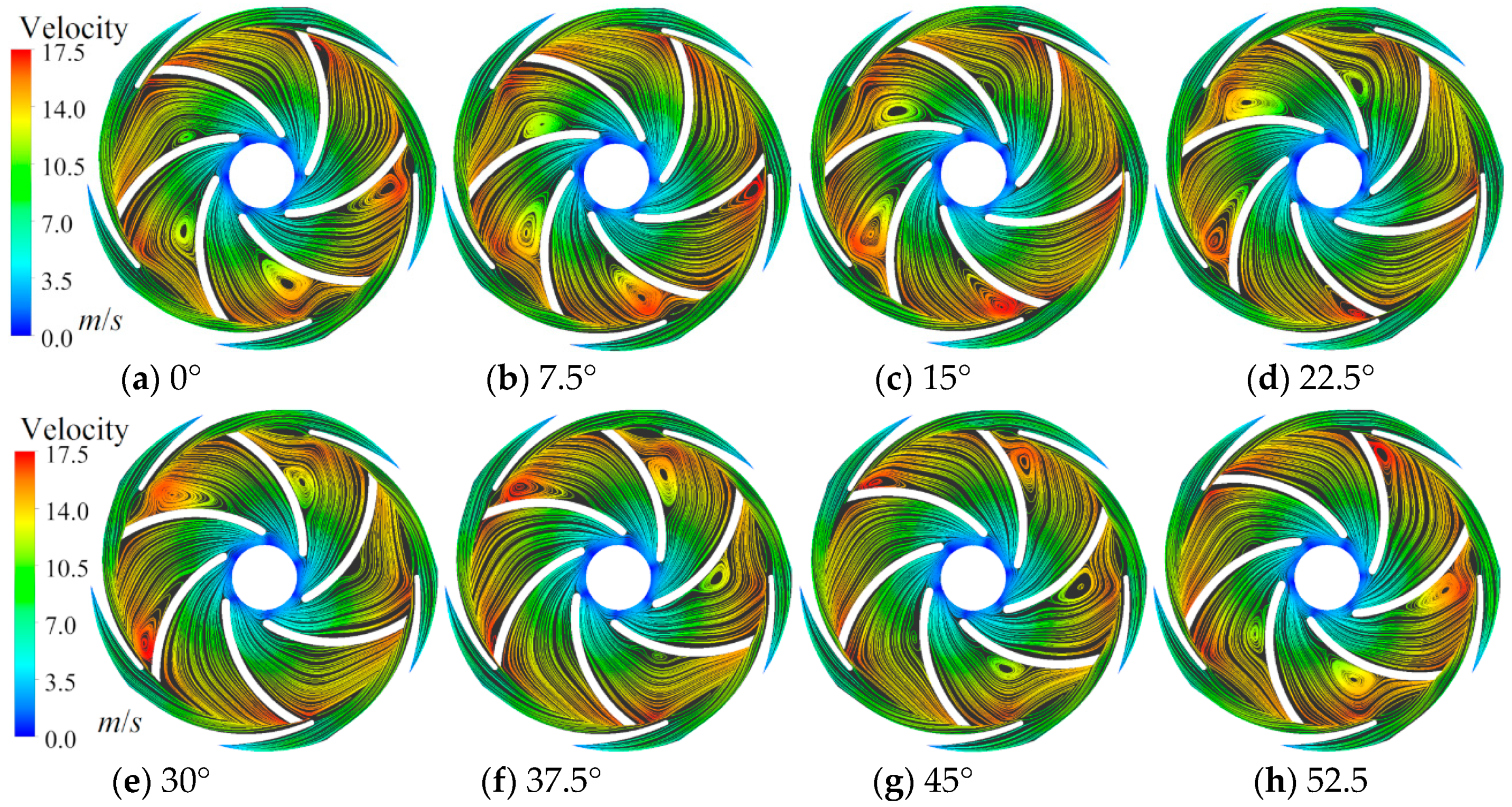
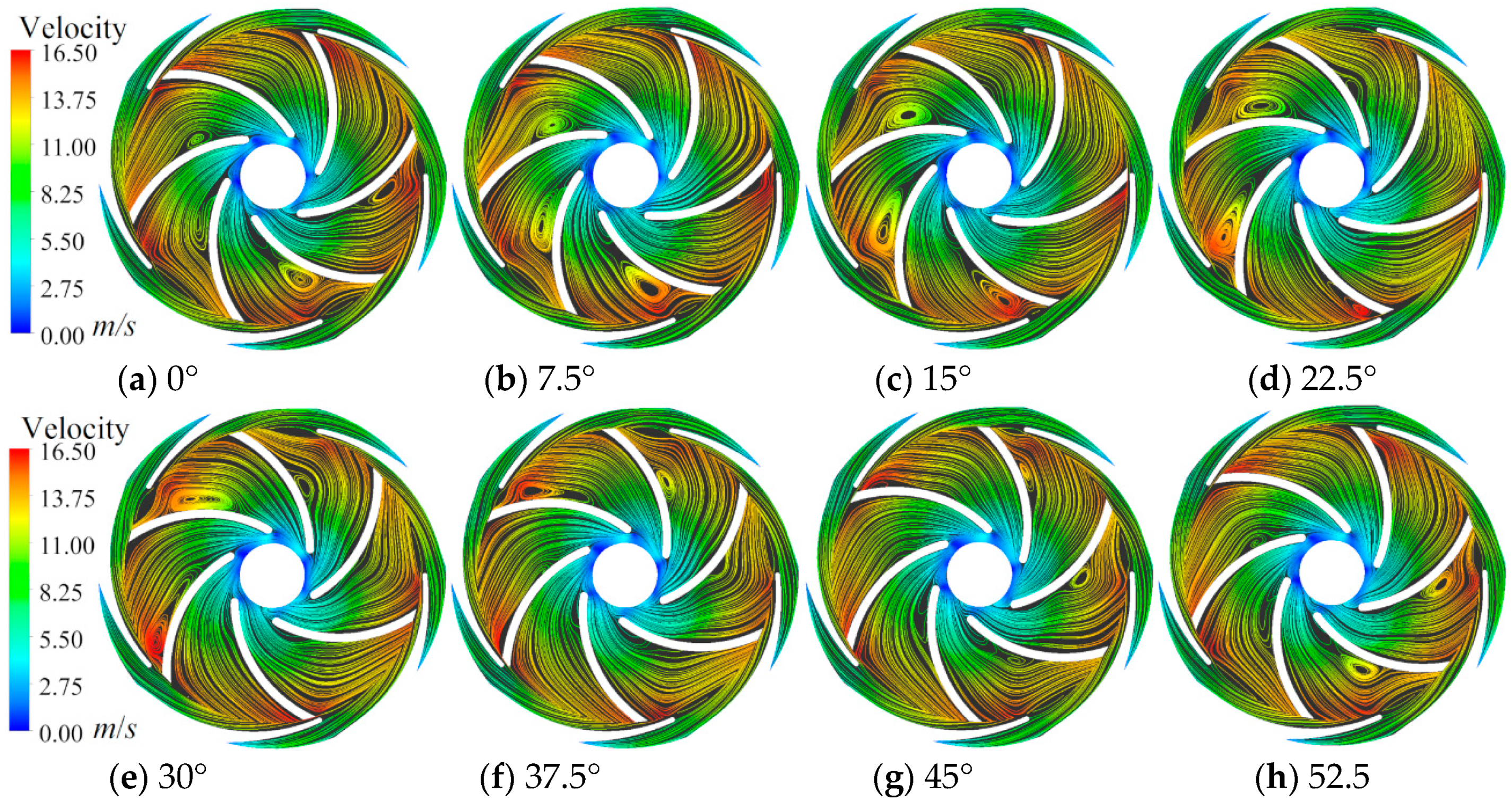
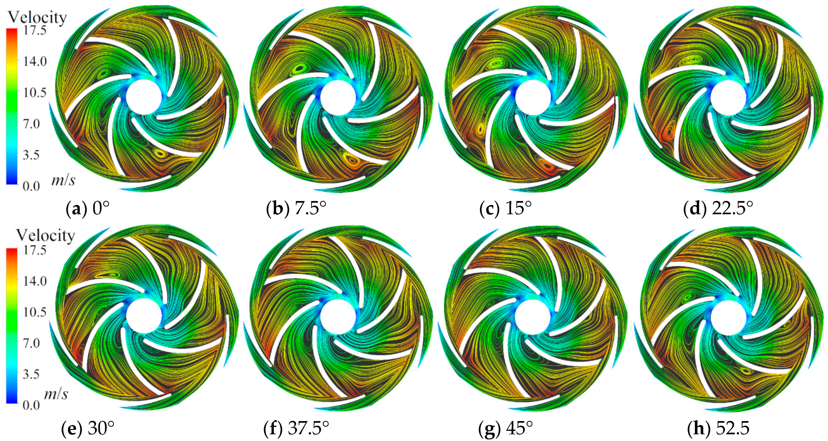
To understand the formation mechanism of the unsteady characteristics of the flow field in the JCP, in this section, the formation and evolution process of vortices in the impeller and guide vane of the JCP under four conditions is studied by a transient analysis method. Figure 11, Figure 12, Figure 13 and Figure 14 show the spatial and temporal evolution processes of the vortices in the stator and rotor cascades during a 1/6 cycle (60 degrees) of impeller rotation under four conditions. Since the impeller of the model pump contains six blades evenly arranged in the circumferential direction, a 1/6 cycle of the flow process actually reflects the transient flow characteristics of the pump during the whole operating period.
It can be seen that the vortices in every impeller passage underwent a process from generation to disappearance in each operating condition within 1/6 of a cycle, but the intensity and pattern of the vorticity were unique in different passages and time. This is because, on the one hand, the number of impeller and guide vane blades was different, and on the other hand, from the velocity vector and streamline analysis of the pump chamber in the previous section, there is flow asymmetry in the upper, lower, left, and right parts of the pump chamber. The process from generation to disappearance of the vortices is related to the constant change of the relative positions of the impeller blades and guide vane blades. When the outlet flow in a channel of the impeller is divided by a guide vane and flows into two adjacent guide vane channels, backflow and vorticity will arise in the impeller outlet near the pressure surface. When a vortex exists in the impeller channel, blockage of the flow path will occur in the inlet of the guide vane. The more obvious the vortex is, the more serious the blockage, which will affect the normal and steady flow in the guide vane. By comparing the vortex evolution processes under different conditions, it can be seen that the smaller the flow rate of the pump, the more obvious the vortices and the more serious the blockage of the flow passage, but their evolution law is basically the same. The above analysis results show that the temporal and spatial evolution processes and law of vortices in the rotor and stator cascades are closely related to the relative positions of the impeller blades and the guide vane blades. Therefore, the design of impeller or guide vane geometry and the optimization of the internal flow field of JCPs should focus on the overall matching of rotor and stator cascades.
6. Pressure Fluctuation Characteristics of the Main Flow Passage Components
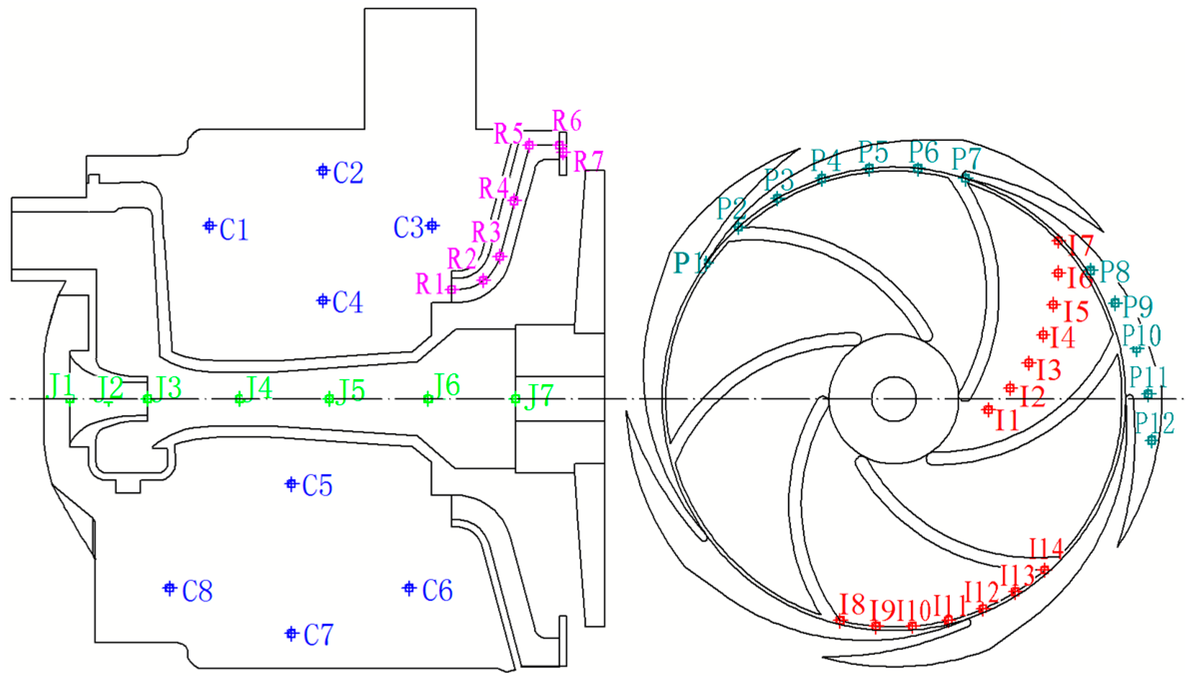
In this section, we analyze in the time and frequency domains the pressure fluctuation characteristics of the flow field inside the main flow passage components of the model pump under the rated operating conditions. Figure 15 shows a schematic diagram of the positions of the monitoring points in each component.
6.1. Impeller
6.1.1. Monitoring Points Stationary Relative to the Fixed Coordinate System
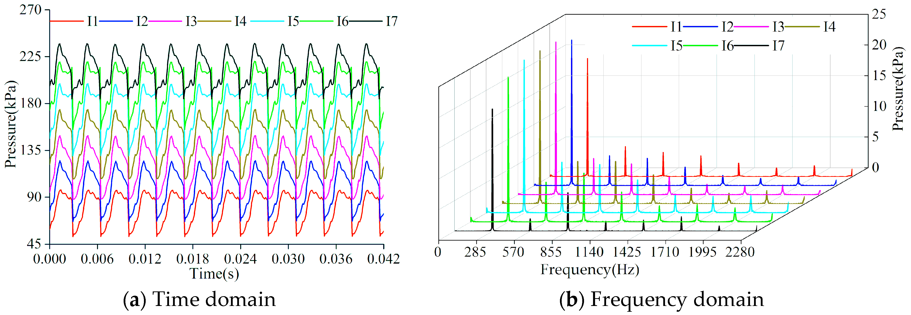
Figure 16 shows the time and frequency domain diagrams of pressure fluctuation for the monitoring points at the middle streamline of a single impeller channel when the monitoring points are stationary relative to the fixed coordinate system. The time domain diagram is the variation curve over two impeller rotation cycles (the same is true below). It can be seen that when the impeller rotates one full circle, the number of pressure fluctuation waves at each monitoring point is consistent with the number of impeller blades—six similar periodic waveforms. From Figure 16b, we can see that the dominant frequency of pressure fluctuation at each monitoring point is BPFI, and it has obvious amplitudes at other low-order frequency multiplications of BPFI. Along the direction of radius increase, the pressure fluctuation curves rise overall, but the fluctuation amplitude does not change much.
6.1.2. Monitoring Points Stationary Relative to the Rotating Coordinate System
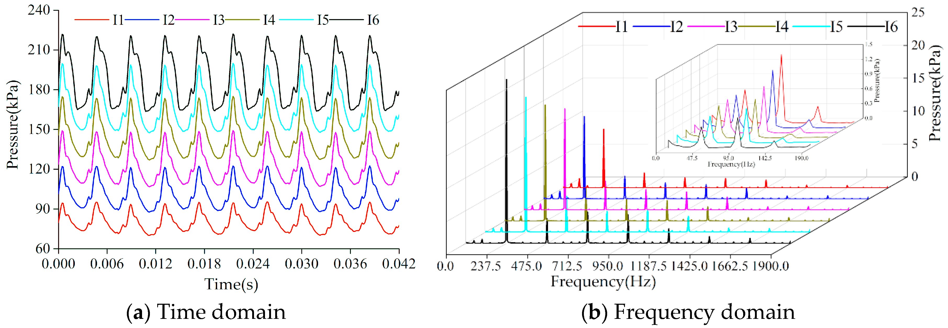
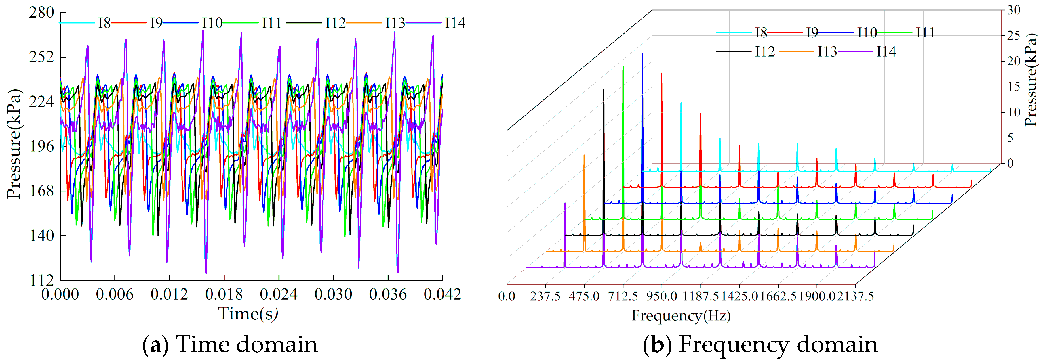
Figure 17 shows the time and frequency domain diagrams of pressure fluctuation for the monitoring points at the middle streamline of a single impeller passage when the monitoring points are stationary relative to the rotating coordinate system. From Figure 17a, it can be seen that there are five obvious similar waveforms at each monitoring point when the impeller rotates one full cycle, which is consistent with the number of guide vanes (of which there are five). The pressure fluctuation curve at each monitoring point rises overall with the radius, but the law of variation with time is basically the same. Figure 17b shows that the dominant frequency of pressure fluctuation at all the monitoring points is 237.5 Hz, which is the BPFG, and obvious amplitudes appear at low-order frequency multiplications of the dominant frequency. As the monitoring point gets closer to the impeller outlet, the rotor and stator interference becomes more and more violent, so the fluctuation amplitude at each characteristic frequency becomes larger and larger. In addition, relatively small fluctuation amplitudes are also shown at the shaft-passing frequency and its multiplication frequency, which reflects the influence of the impeller operating parameters (pump rotation speed) on the unsteady flow field of the JCP.
Figure 18 shows the time and frequency domain diagrams of pressure fluctuation for monitoring points at the outlet edge of a single impeller channel. It can be seen from Figure 18a that when the impeller rotates one full circle, the pressure fluctuates five times, which is consistent with the number of guide vanes. However, the variation law with time is different: peaks and troughs occur at different times because the pressure fluctuation in the impeller is closely related to the relative positions of the guide vanes, and the guide vanes pass the monitoring point one by one, so the wave peaks or troughs appear in turn. Figure 18b shows that the dominant frequency of pressure fluctuation for all of the points is BPFG, and there are obvious amplitudes at low-order frequency multiplications of BPFG. At the dominant frequency, the fluctuation amplitude in the middle region of the flow channel is larger, while that at the points near the pressure or suction surface is relatively small.
The analysis results from Figure 16, Figure 17 and Figure 18 show that the pressure fluctuation characteristics of the impeller flow field are mainly related to the number of impeller blades and the speed of the impeller when the monitoring points are stationary relative to the fixed coordinate system. The pressure fluctuation characteristics of the impeller flow field are determined by the number of guide vane blades and the speed of the impeller when the monitoring points are stationary relative to the rotating coordinate system, and the farther the monitoring point is from the interface of the rotor and stator cascades, the weaker the fluctuation amplitude at the characteristic frequencies.
6.2. Guide Vane
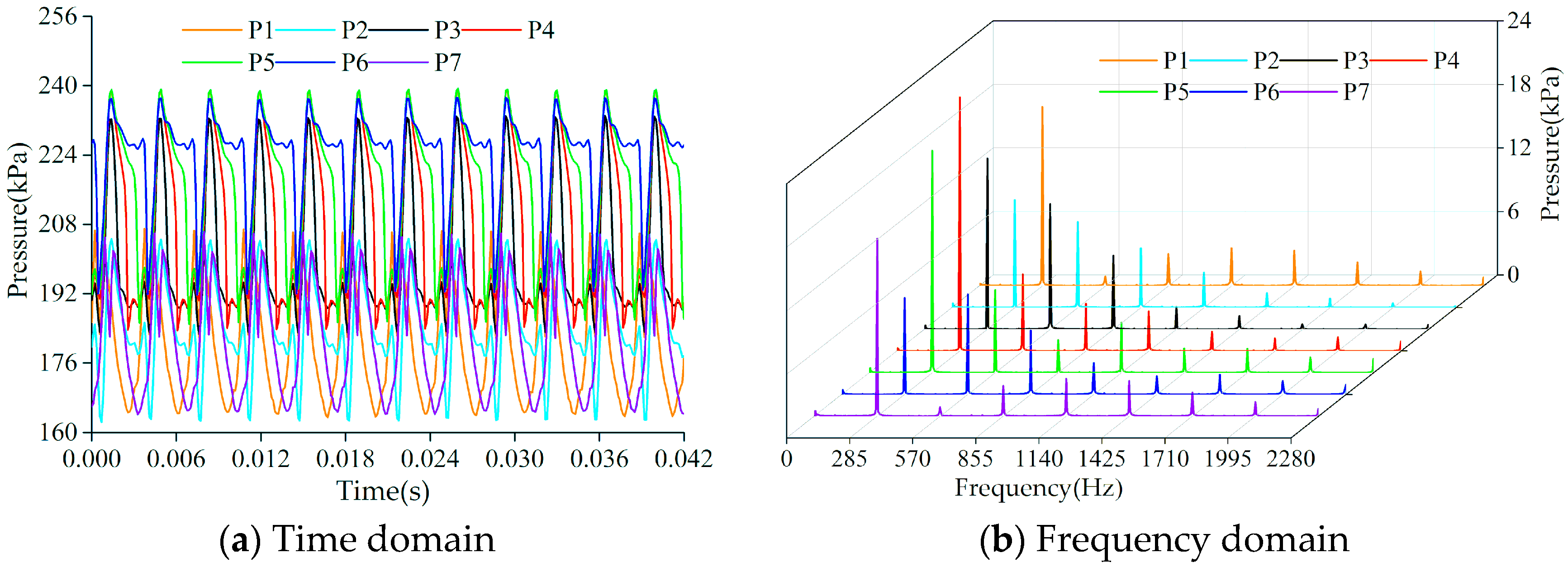
Figure 19 shows the time and frequency domain diagrams of the pressure fluctuation characteristics for monitoring points at the inlet edge of a guide vane channel. Figure 19a shows that the pressure fluctuation at each monitoring point exhibits six periods in an impeller cycle, which is consistent with the number of impeller blades, but the variation laws with time are not identical. The times when peaks and troughs appear are different because the pressure fluctuation characteristics in the guide vane channel are closely related to the relative position of the impeller blades. The impeller blades pass the monitoring point one by one, so the wave peaks and troughs at that point appear in turn. Figure 19b shows that the dominant frequency of pressure fluctuation at all the monitoring points is BPFI, and there are obvious amplitudes at low-order frequency multiplications of BPFI.
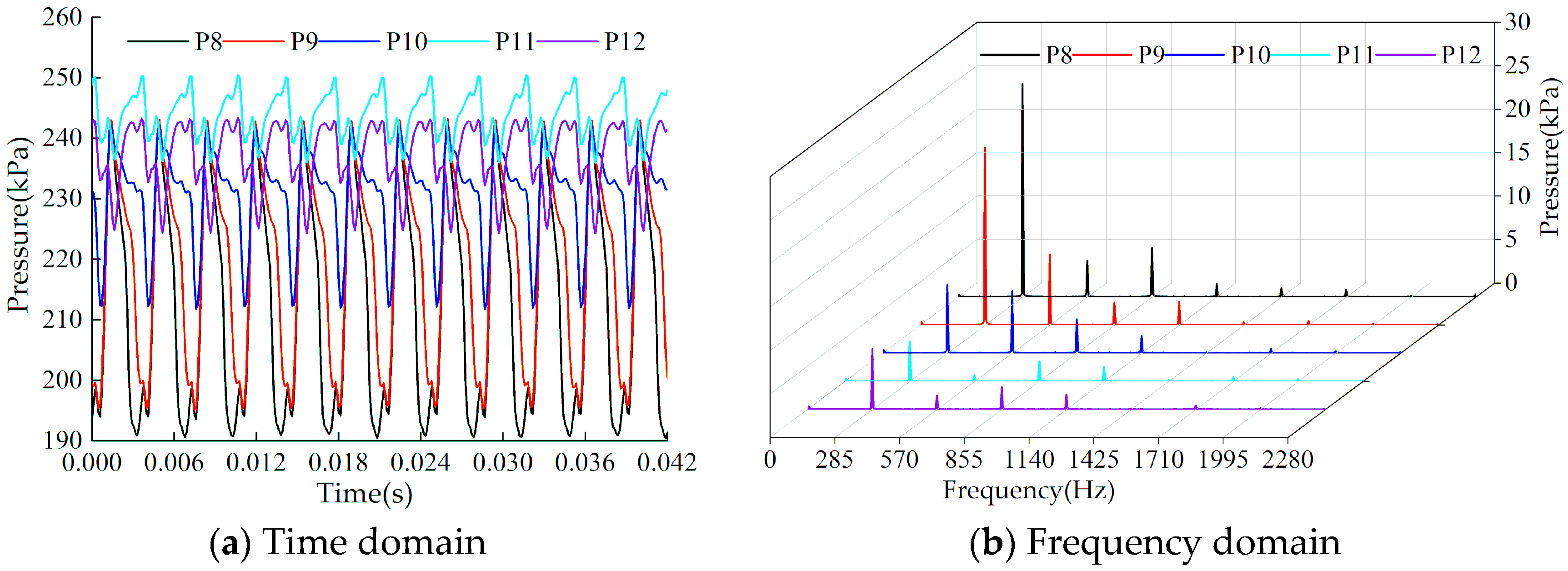
Figure 20 shows the time and frequency domain diagrams of the pressure fluctuation characteristics for monitoring points at the single-channel middle streamline of the guide vane. Figure 20a shows that the time domain characteristic curve of pressure fluctuation is related to the number of impeller blades. As the radius increases, the average pressure at each monitoring point increases as a whole, but it decreases at the outlet position of the positive guide vane; this is due to the gradual transition of the flow direction from the radial to the axial direction. Figure 20b shows that the dominant frequency of the pressure fluctuation is BPFI, and there are amplitudes at other frequency multiplications of BPFI. As the radius increases, the influence of the impeller on the guide vane gradually weakens, so the amplitude, in turn, decreases at characteristic frequencies, but it rises slightly at the outlet of the positive guide vane, where the flow is complex.
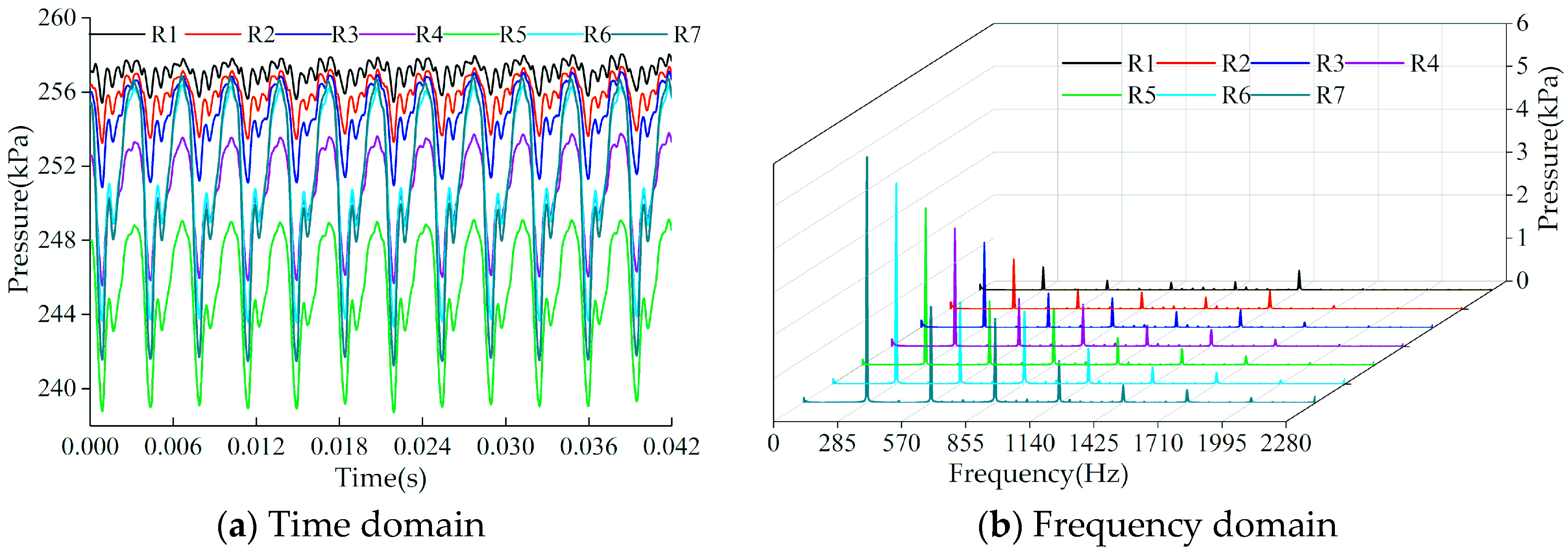
Figure 21 shows the time and frequency domain diagrams of the pressure fluctuation characteristics for monitoring points at the middle streamline of a return guide vane channel. Figure 21a shows that the fluctuation characteristics of the pressure inside the return guide vane in the time domain are basically the same as those of the positive guide vane. After the fluid passes through the monitoring point R5, the average pressure increases gradually along the outlet direction. Figure 21b shows that the characteristic frequencies of pressure fluctuation are BPFI and its low-order frequency multiplications, among which the dominant frequency is BPFI along the outlet direction. The amplitude of pressure fluctuation at the dominant frequency and other characteristic frequencies decreases monotonically, which is due to the influence of rotor–stator interaction becoming weaker and weaker as the monitoring point is farther away from the impeller.
The analysis results of Figure 19, Figure 20 and Figure 21 show that the pressure fluctuation characteristics of the fluid in the guide vane are mainly related to the number of impeller blades and impeller speed. The farther the monitoring point is from the interface of the rotor and stator cascades, the weaker the fluctuation amplitude at the characteristic frequency.
6.3. Pump Chamber and Ejector
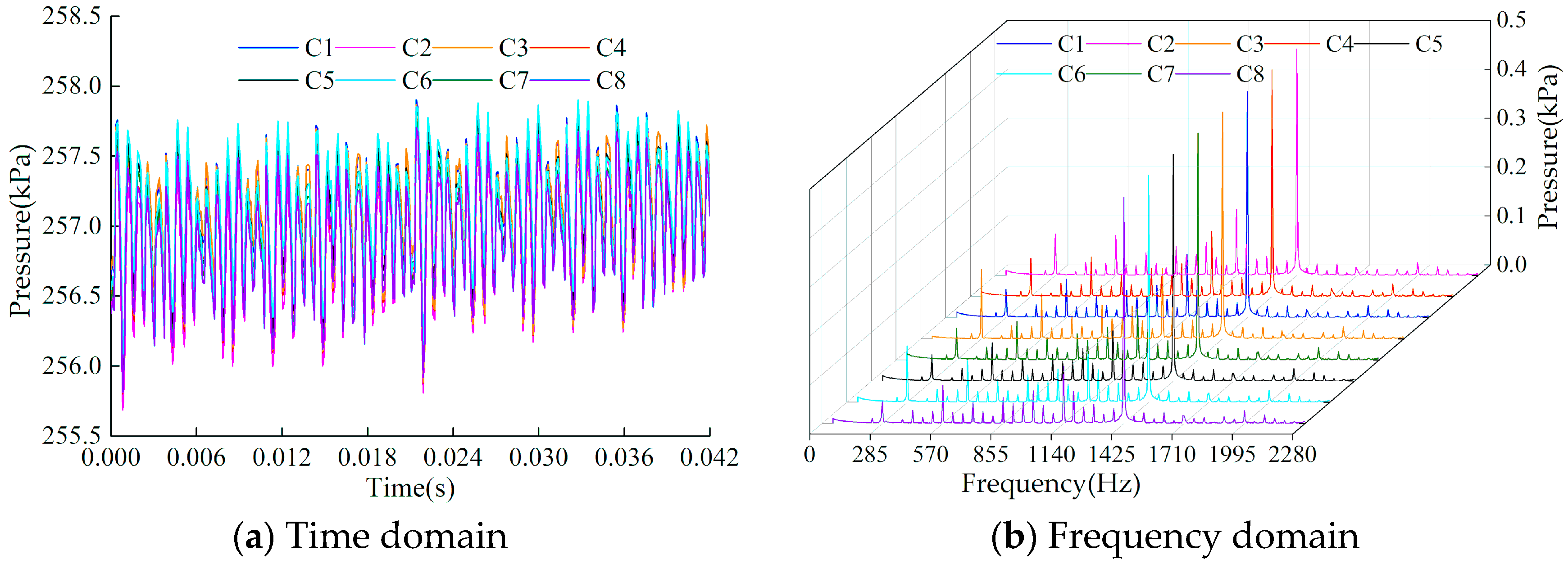
Figure 22 shows the time and frequency domain diagrams of the pressure fluctuation characteristics for monitoring points in the pump chamber. Figure 22a shows that the pressure at the monitoring points in the pump chamber presents obvious periodic fluctuation characteristics in the time domain, and their fluctuation ranges and variation laws are very consistent. In a rotation period of the impeller, the pressure fluctuation has 30 peaks and troughs, which is the product of the number of impeller blades and the number of guide vane blades. Figure 22b shows that the amplitude of pressure fluctuation inside the pump chamber is obviously smaller than that at the impeller and guide vane, which is consistent with the analysis results of the pressure fluctuation intensity in Section 4.2. The dominant frequency of pressure fluctuation at each monitoring point is 1425 Hz, which is the frequency of the rotor and stator cascade encounter (impeller speed × impeller blade number × guide vane blade number). The difference in fluctuation amplitude is small among the different monitoring points at the dominant frequency and at the other characteristic frequencies. In addition, there are obvious fluctuation amplitudes when the frequency of the SPF doubles, which have an important influence on the unsteady fluctuation characteristics of the pump chamber.
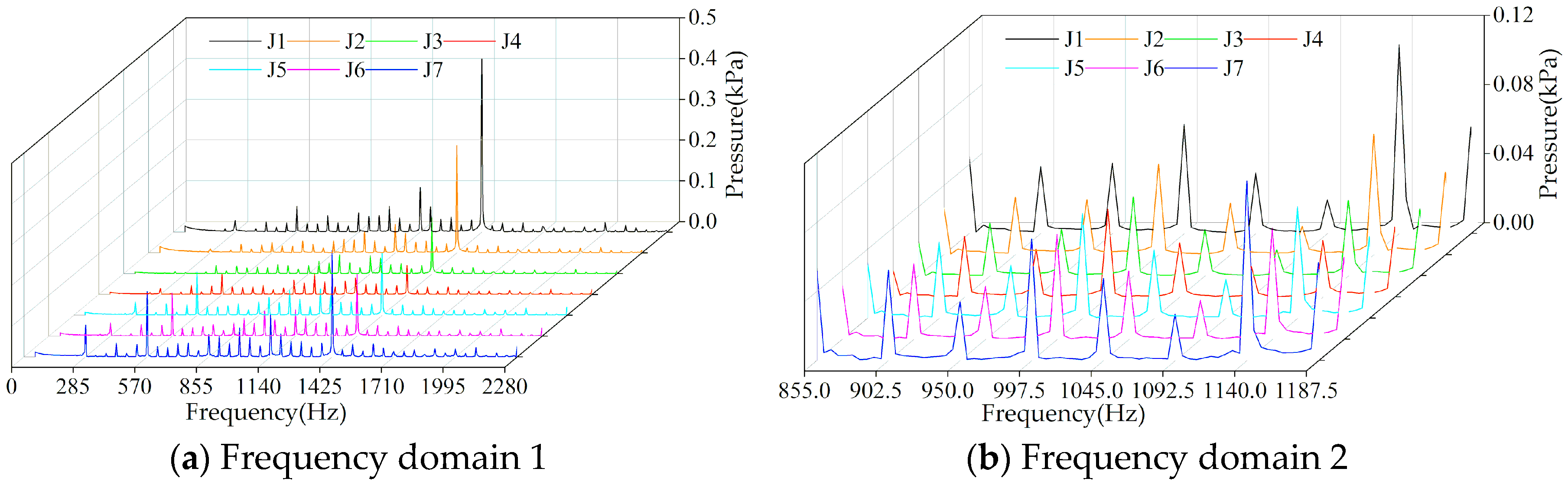
Figure 23 is the frequency domain diagram of the pressure fluctuation characteristics for the monitoring points in the ejector nozzle and tube. It can be seen that the pressure fluctuation characteristics of the flow field in the ejector are basically the same as those in the pump chamber. That is, the dominant frequency is the encounter frequency of the rotor and stator cascades. Within the ejector nozzle, the fluctuation amplitude at the dominant frequency decreases gradually along the flow direction. The closer the monitoring point is to the impeller, the greater the pressure fluctuation amplitude. It can be seen from Figure 23b that there are non-negligible fluctuation amplitudes at frequency multiplications of the SPF.
The analysis results of Figure 22 and Figure 23 show that the pressure fluctuation characteristics of the flow field in the pump chamber and ejector are the result of combined action, including the interaction of the number of impeller blades, the number of guide vane blades, and the speed of the impeller. The rotor–stator interaction affects not only the unsteady flow characteristics in the impeller and guide vanes, but also the pump chamber and ejector.
7. Conclusions
In this paper, the transient fluctuation characteristics of a flow field in the major flow passage components of a jet centrifugal pump, and the spatial and temporal evolution laws of vortices in rotor–stator cascades were analyzed. The main results are as follows:
(1) Under multiple operating conditions, various scales of flow distortion phenomena occur in the JCP chamber, such as eddies, blockage of the flow passage, recirculation, secondary flow, and circulation, which not only cause great hydraulic loss, but also destroy the flow stability, symmetry, and balance of the other flow passage components’ flow fields. This is an important reason for the obviously lower efficiency of JCPs than that of general centrifugal pumps.
(2) The spatial and temporal evolution laws of vortices in rotor–stator cascades are mainly related to the relative positions of impeller blades and guide vane blades; the scale of vortices is not only related to the structures of the impeller blade and guide vane blade, but also to their matching relationship. Therefore, the design of impeller or guide vane geometry and the optimization of the internal flow field of a JCP should focus on the overall matching of rotor and stator cascades.
(3) The pressure fluctuation characteristics in the impeller are mainly determined by the number of guide vane blades and the pump rotation speed; those in the guide vane by the number of impeller blades and the pump rotation speed; and those in the pump chamber and ejector by the numbers of impeller blades and guide vane blades and the pump rotation speed. All of this reflects that the formation mechanism of the unsteady flow field fluctuation characteristics of a JCP is mainly related to the number of blades in the rotor–stator cascades and the operation parameters of the pump.
(4) The fluctuation intensity of the flow field inside the impeller and guide vane is obviously greater than that in other flow areas, reflecting that rotor–stator interaction is the decisive factor affecting the unsteady flow characteristics of a JCP under multiple conditions.
Author Contributions
Formal analysis, R.G.; Funding acquisition, R.L.; Methodology, R.G.; Resources, R.Z.; Validation, W.H.; Writing—original draft, R.G.; Writing—review and editing, R.L.
Funding
This research was funded by Natural Science Foundation of China, grant number 51579125; National Key Research and Development Program of China, grant number 2016YFB0200901.
Acknowledgments
The authors gratefully acknowledge the financial support from the National Natural Foundation of China (51579125) and the National Key Research and Development Program of China (2016YFB0200901).
Conflicts of Interest
The authors declare no conflict of interest.
Nomenclature
| Qd | Rated volume flow m3/h |
| Hd | Rated water head m |
| ηd | Rated efficiency % |
| n | Rotational speed r/min |
| SPF | Shaft passing frequency Hz |
| BPFI | Blade passing frequency of impeller Hz |
| BPFG | Blade passing frequency of guide vane Hz |
| Dj | Inlet diameter of impeller mm |
| D2 | Outlet diameter of impeller mm |
| Z1 | Blade number of impeller |
| φ1 | Blade wrap angle of impeller ° |
| b2 | Blade outlet width of impeller mm |
| D3 | Base diameter of guide vane mm |
| D4 | Outlet diameter of guide vane mm |
| Z2 | Blade number of guide vane |
| GGI | General grid interface |
| Time-averaged components | |
| Periodic components | |
| n | Grid nodes |
| N | Number of samples in an impeller rotating period |
| t | Total time |
| t0 | Starting time of the rotation cycle |
| Non-dimensional pressure fluctuation intensity | |
| Non-dimensional velocity fluctuation intensity | |
| Non-dimensional turbulence energy fluctuation intensity | |
| Pressure fluctuation intensity | |
| Velocity fluctuation intensity | |
| Turbulence energy fluctuation intensity |
References
- Liu, J.R.; Zhou, G.P. Research and prospects for the self-priming irrigation pumps. Trans. Chin. Soc. Agric. Mach. 2007, 8, 177–180. [Google Scholar] [CrossRef]
- Wang, W.J.; Tang, Y.; Ma, H.; Yang, Z. Design and research of jet self-priming centrifugal pump. Equip. Manuf. Technol. 2017, 5, 32–34. [Google Scholar]
- Li, W.; Chang, H.; Liu, J.R.; Zhou, L.; Wang, C. Research situation and prospect of jet type self-priming centrifugal pump. Drain. Irrig. Mach. Eng. 2016, 34, 947–952. [Google Scholar] [CrossRef]
- Wang, C.; Hu, B.; Zhu, Y.; Wang, X.L.; Luo, C.; Cheng, L. Numerical study on the gas-water two-phase flow in the self-priming process of self-priming centrifugal pump. Processes 2019, 7, 330. [Google Scholar] [CrossRef]
- Wang, Y.; Li, G.D.; Cao, P.Y.; Yin, G.; Cui, Y.R.; Li, Y.C. Effects of internal circulation flow on self-priming performance of flow-ejecting self-priming pump. Trans. Chin. Soc. Agric. Mach. 2014, 45, 129–133. [Google Scholar] [CrossRef]
- Wang, Y.; Han, Y.W.; Zhu, X.X.; Sun, W.; Cao, P.Y.; Wu, W. Optimization and experiment on performance of flow-ejecting self-priming pump based on CFD. Trans. Chin. Soc. Agric. Eng. 2016, 32, 16–21. [Google Scholar] [CrossRef]
- Liu, J.R.; Wen, H.G.; Gao, Z.J.; Guo, C.X.; Wang, P. Effects of geometric parameters for jet nozzle on self-priming performance of spray pump. Trans. Chin. Soc. Agric. Eng. 2012, 28, 47–54. [Google Scholar] [CrossRef]
- Liu, J.R.; Wen, H.G.; Xiang, H.J.; Guo, C.X.; Gao, Z.J. Effects of diffuser on self-priming performance of flow-ejecting self-priming centrifugal pump. Trans. Chin. Soc. Agric. Mach. 2013, 44, 43–47. [Google Scholar] [CrossRef]
- Wang, C.; Shi, W.D.; Li, W.; Zhang, D.S.; Jiang, X.P. Unsteady numerical calculation and validation on self-priming process of self-priming spray irrigation pump. Trans. Chin. Soc. Agric. Eng. 2016, 32, 65–72. [Google Scholar] [CrossRef]
- Zhang, R.H.; Zhang, S.D.; Tian, L.; Chen, X.B. Research on performance and inner flow characteristics of jet centrifugal pump. J. Drain. Irrig. Mach. Eng. 2019, 37, 763–768+775. [Google Scholar] [CrossRef]
- Chen, N.; Liu, W.H.; Lai, H.Q. Numerical analysis of flow field inside injection pump by CFD. Ship Sci. Technol. 2016, 38, 53–56. [Google Scholar] [CrossRef]
- Li, G.D.; Wang, Y.; Yang, X.M.; Zhao, L.F.; Wu, W.; Hu, R.X. Features of internal flow in jet nozzle of self-priming centrifugal pump based on large eddy simulation. J. Drain. Irrig. Mach. Eng. 2017, 35, 369–374. [Google Scholar] [CrossRef]
- Wang, Y.; Cui, Y.R.; Wang, K.; Wang, W.J.; Li, G.D.; Yin, G. Analysis of unsteady flow in flow-ejecting self-priming centrifugal pump based on LES. J. Drain. Irrig. Mach. Eng. 2015, 33, 481–487. [Google Scholar] [CrossRef]
- Wang, W.J.; Wang, Y.; Li, G.D.; Yin, G.; Cao, P.Y. Numerical simulation and testing analysis of three dimensional turbulence flow in flow-ejecting self-priming centrifugal pump. Trans. Chin. Soc. Agric. Mach. 2014, 45, 54–60. [Google Scholar] [CrossRef]
- Li, G.D.; Wang, Y.; Cao, P.Y.; Zhou, G.H.; Wu, W.; Han, Y.W. Internal flow of flow-ejecting centrifugal pump under off-design conditions. Trans. Chin. Soc. Agric. Mach. 2015, 46, 48–53. [Google Scholar] [CrossRef]
- Ansys Inc. Ansys Fluent Theory Guide; Ansys Inc.: Canonsburg, PA, USA, 2015. [Google Scholar]
- Pei, J.; Yuan, S.Q.; Yuan, J.P.; Wang, W.J. Comparative study of pressure fluctuation intensity for a single blade pump under multiple operating conditions. J. Huazhong Univ. Sci. Technol. 2013, 41, 29–33. [Google Scholar] [CrossRef]
Figure 1.
Structural diagrams of the model pump. (a) Two-dimensional structure diagram; (b) Three-dimensional structure diagram. 1: Ejector nozzle; 2: Ejector; 3: Pump chamber; 4: Ejector tube; 5: Guide vane; 6: Impeller; 7: Pump cover.
Figure 1.
Structural diagrams of the model pump. (a) Two-dimensional structure diagram; (b) Three-dimensional structure diagram. 1: Ejector nozzle; 2: Ejector; 3: Pump chamber; 4: Ejector tube; 5: Guide vane; 6: Impeller; 7: Pump cover.

Figure 2.
Grid diagrams of the impeller, guide vane, and jet. (a) Impeller; (b) Guide vane; (c) Ejector nozzle and tube.
Figure 2.
Grid diagrams of the impeller, guide vane, and jet. (a) Impeller; (b) Guide vane; (c) Ejector nozzle and tube.

Figure 3.
Experimental system and result. (a) Experimental system; (b) A comparison of hydraulic performance between the experiment and the numerical simulation. 1: Valve at pump outlet; 2: Flowmeter; 3: Pressure sensor at pump outlet; 4: The model pump; 5: Electric motor; 6: Pressure sensor at pump inlet; 7: Tachometer; 8: Valve at pump inlet; 9: Computer; 10: Measuring instrument of electric power.

Figure 4.
Velocity vector and streamline diagrams under different working conditions.

Figure 5.
Time-averaged distribution contours of pressure on two planes under four conditions.

Figure 6.
Time-averaged distribution contours of absolute velocity on two planes under four conditions.
Figure 6.
Time-averaged distribution contours of absolute velocity on two planes under four conditions.

Figure 7.
Time-averaged distribution contours of turbulent kinetic energy on two planes under four conditions.
Figure 7.
Time-averaged distribution contours of turbulent kinetic energy on two planes under four conditions.

Figure 8.
Fluctuation intensity distribution contours of pressure on two planes under four conditions.
Figure 8.
Fluctuation intensity distribution contours of pressure on two planes under four conditions.

Figure 9.
Fluctuation intensity distribution contours of velocity on two planes under four conditions.
Figure 9.
Fluctuation intensity distribution contours of velocity on two planes under four conditions.

Figure 10.
Fluctuation intensity distribution contours of velocity on two planes under four conditions.
Figure 10.
Fluctuation intensity distribution contours of velocity on two planes under four conditions.


Figure 11.
Evolution processes of the vortices in the stator and rotor cascade during a 1/6 period of impeller rotation under condition 0.2 Qd.
Figure 11.
Evolution processes of the vortices in the stator and rotor cascade during a 1/6 period of impeller rotation under condition 0.2 Qd.

Figure 12.
Evolution processes of the vortices in the stator and rotor cascade during a 1/6 period of impeller rotation under condition 0.6 Qd.
Figure 12.
Evolution processes of the vortices in the stator and rotor cascade during a 1/6 period of impeller rotation under condition 0.6 Qd.

Figure 13.
Evolution processes of the vortices in the stator and rotor cascade during a 1/6 period of impeller rotation under condition 1.0 Qd.
Figure 13.
Evolution processes of the vortices in the stator and rotor cascade during a 1/6 period of impeller rotation under condition 1.0 Qd.

Figure 14.
Evolution processes of the vortices in the stator and rotor cascade during a 1/6 period of impeller rotation under condition 1.4 Qd.
Figure 14.
Evolution processes of the vortices in the stator and rotor cascade during a 1/6 period of impeller rotation under condition 1.4 Qd.

Figure 15.
A schematic diagram of the positions of the monitoring points in each component.

Figure 16.
The time and frequency domain diagrams of pressure fluctuation for the monitoring points at the middle streamline of a single impeller channel when the monitoring points are stationary relative to the fixed coordinate system.
Figure 16.
The time and frequency domain diagrams of pressure fluctuation for the monitoring points at the middle streamline of a single impeller channel when the monitoring points are stationary relative to the fixed coordinate system.

Figure 17.
The time and frequency domain diagrams of pressure fluctuation at monitoring points on the middle streamline of a single impeller channel when the monitoring points are stationary relative to the rotational coordinate system.
Figure 17.
The time and frequency domain diagrams of pressure fluctuation at monitoring points on the middle streamline of a single impeller channel when the monitoring points are stationary relative to the rotational coordinate system.

Figure 18.
The time and frequency domain diagrams of pressure fluctuation for the monitoring points at the outlet edge of a single impeller channel.
Figure 18.
The time and frequency domain diagrams of pressure fluctuation for the monitoring points at the outlet edge of a single impeller channel.

Figure 19.
The time and frequency domain diagrams of pressure fluctuation for monitoring points at the inlet edge of a guide vane channel.
Figure 19.
The time and frequency domain diagrams of pressure fluctuation for monitoring points at the inlet edge of a guide vane channel.

Figure 20.
The time and frequency domain diagrams of pressure fluctuation for monitoring points at the middle streamline of a guide vane channel.
Figure 20.
The time and frequency domain diagrams of pressure fluctuation for monitoring points at the middle streamline of a guide vane channel.

Figure 21.
The time and frequency domain diagrams of pressure fluctuation for monitoring points at the middle streamline of a return guide vane channel.
Figure 21.
The time and frequency domain diagrams of pressure fluctuation for monitoring points at the middle streamline of a return guide vane channel.

Figure 22.
The time and frequency domain diagrams of pressure fluctuation for monitoring points in the pump chamber.
Figure 22.
The time and frequency domain diagrams of pressure fluctuation for monitoring points in the pump chamber.

Figure 23.
Frequency domain diagrams of pressure fluctuation for monitoring points in the ejector.


Table 1.
Parameters of the model jet centrifugal pump.
| Parameter | Value | |
|---|---|---|
| Impeller | Inlet Diameter Dj (mm) | 40 |
| Outlet Diameter D2 (mm) | 123 | |
| Blade Number Z1 | 6 | |
| Blade Wrap Angle φ (°) | 76 | |
| Blade Outlet Width b2 (mm) | 5.3 | |
| Guide Vane | Base Diameter (mm) | 125 |
| Outlet Diameter D3 (mm) | 64 | |
| Blade Number Z2 | 5 |
Table 2.
The grid independence analyzation.
| Schemes | Scheme 1 | Scheme 2 | Scheme 3 | Scheme 4 | Scheme 5 | Scheme 6 |
|---|---|---|---|---|---|---|
| Number of the grid | 1,483,718 | 1,975,598 | 2,526,764 | 3,030,389 | 3,494,674 | 4,046,652 |
| Head (m) | 23.97 | 24.22 | 25.43 | 26.15 | 26.17 | 26.16 |
© 2019 by the authors. Licensee MDPI, Basel, Switzerland. This article is an open access article distributed under the terms and conditions of the Creative Commons Attribution (CC BY) license (http://creativecommons.org/licenses/by/4.0/).
Share and Cite
MDPI and ACS Style
Guo, R.; Li, R.; Zhang, R.; Han, W. Numerical Study of the Unsteady Flow Characteristics of a Jet Centrifugal Pump under Multiple Conditions. Processes 2019, 7, 786. https://doi.org/10.3390/pr7110786
AMA Style
Guo R, Li R, Zhang R, Han W. Numerical Study of the Unsteady Flow Characteristics of a Jet Centrifugal Pump under Multiple Conditions. Processes. 2019; 7(11):786. https://doi.org/10.3390/pr7110786
Chicago/Turabian StyleGuo, Rong, Rennian Li, Renhui Zhang, and Wei Han. 2019. "Numerical Study of the Unsteady Flow Characteristics of a Jet Centrifugal Pump under Multiple Conditions" Processes 7, no. 11: 786. https://doi.org/10.3390/pr7110786
Note that from the first issue of 2016, this journal uses article numbers instead of page numbers. See further details here.