Optimal Design of Perforated Diversion Wall Based on Comprehensive Evaluation Indicator and Response Surface Method: A Case Study

Abstract

To investigate the impact of parameters of diversion wall holes on the flow state in the forebay of a combined sluice-pumping station project and optimize the relevant parameters, a total of 50 numerical simulations based on the CFD technique were performed, adopting the design of orthogonal experiments with 25 schemes under self-draining conditions and pumping conditions, respectively. For synthesizing flow state evaluation indicators under self-draining and pumping conditions, the variation coefficient method was used, and the results were analyzed through the response surface method. Thus, the relationship between the parameters of the diversion wall holes and the comprehensive evaluation indicator was established. The steepest ascent method was used to obtain the optimal parameters, and the results showed that the optimized holes can balance the flow state under self-draining and pumping conditions in the combined sluice-pumping station project. Compared to the case with the diversion wall unperforated, the uniformity of axial velocity distribution in the 6# inlet channel and 7# sluice chamber increased by 6.6% and 5.2%, respectively, and the maximum transverse velocity decreased from 0.32 m/s to 0.21 m/s, with a fall of 34.4%. This study provides reference and technical support for the hydraulic characteristic analysis, optimization design and rectifying measures selection of the combined sluice-pumping station project.

1. Introduction

The combined sluice-pumping station has advantages such as a small footprint and low construction and management costs. However, a significant disadvantage of the system is that it significantly differs in flow regimes under different operating conditions, which are consistently unsatisfactory. When the sluice or pumping station operates independently, the flow direction of the water is not aligned with the riverbed, which leads to an imbalance in the momentum of the two sides of the riverbed. As a result, backflow, whirlpools, oblique flow and transverse flow occur, which reduces the flow capacity of the sluice and the effectiveness of the pumping station [1]. Moreover, from the perspective of security and reliability while the pumping station is in operation, adverse flow patterns can significantly impact the flow in the inlet pool of the pumping station and alter the direction of water into the pump, which leads to the phenomena of cavitation and vibration [2,3,4,5,6]. With respect to the operation of the sluice in isolation, the asymmetry of the backflow can reduce the flow capacity of the sluice, posing a threat to the safety of the building [7,8,9,10]. If these problems cannot be solved effectively, the social and economic benefits of the combined sluice-pumping station project will be greatly reduced. Therefore, hydraulic characteristics analysis and optimal design research of inlet structures in combined sluice-pumping stations have important theoretical significance and engineering application value.

At present, some scholars have carried out a series of studies on hydraulic characteristics and optimal design methods of inlet structures in combined sluice-pumping stations, and they have obtained many beneficial results. Luo et al. [11,12,13] verified the reliability of numerical simulation results through model experiments and utilized numerical simulation techniques to investigate the adverse flow states existing in different types of pump station forebays and sumps as well as the adjustment and optimization effects of rectification measures on the flow states. By analyzing axial velocity distribution uniformity, velocity-weighted average angle and axial average flow velocity of the sump’s longitudinal profile, the optimal rectification measures were determined. These studies fully demonstrate the importance of numerical simulation in fluid mechanics research and provide a valuable reference for improving the flow state of pump stations. Yang et al. [14] used physical model tests and computational simulations to study the flow pattern in the forebay of a pumping station. They found that the combination plan of a rectifier sill and a diversion wall opening was the most effective way to improve the flow pattern, achieving a reduction rate of the vortex area of over 85% and improving the uniformity of flow rate near and far away from the pumping station. Their research provides an optimal plan to adjust the flow pattern in the forebay of a pumping station, which can improve the efficiency and stability of the pumping station, especially in addressing the technical problems of a poor flow pattern in the forebay internal flow field of a lateral intake pumping station. Wang et al. [15] numerically simulated the flow regime of the sluice-pumping station project in the tidal river section based on the N–S equation and the standard k–ε model. They proposed rectification measures such as extending the diversion wall and installing additional bottom sills and diversion piers, which effectively improved the flow pattern of the forebay. Fu et al. [16] conducted an in-depth discussion on the body shape and suitable length of the diversion wall based on a planar symmetric hydraulics model test of the combined sluice-pumping station, and they concluded that the top of the diversion wall should be higher than the water surface and proposed a range of suitable lengths for the diversion wall. Xu et al. [17,18] conducted a physical model experiment to investigate flow behavior in an asymmetric sluice-pumping system and identified the optimal rectification scheme. Considering the limitations of physical model experiments, Xu et al. [19] further studied the influence of the structural parameters of the diversion wall on the flow field using numerical simulation. They then optimized the structural parameters of the diversion wall using a single-factor progressive analysis method. Xu et al. [20] proposed a Y-shaped settling diversion wall that can adapt its configuration to match the operating conditions of combined sluice-pumping station projects and greatly improve the inflow state under both self-draining and pumping conditions. However, it was also found that the perforated diversion wall was more effective than the Y-shaped settling diversion wall in reducing the flow obliquity on the inlet side of the sluice under self-draining condition in the sluice-pumping station.

In summary, the installation of diversion walls is a common and effective measure to enhance the flow conditions in the forebay of the combined sluice-pumping station project. Changing the parameters of the diversion wall, including location, length, height, angle as well as hole width, spacing and depth can affect the flow conditions on the side of the pumping station as well as the inlet flow pattern and transverse velocity on the side of sluice [19,21]. The majority of current research outcomes regarding the diversion wall in the combined sluice-pumping station project are based on the assumption of some parameter schemes of the diversion wall by numerical simulations and model tests or single-factor optimization carried out one by one according to the length, angle, height, hole width, spacing and depth of the diversion wall, without considering the interaction between the above factors [22,23]. In terms of selecting evaluation indexes for optimization, current optimization studies mostly focus on the improvement of inflow hydrodynamics under pumping conditions as the evaluation indicator and the optimized parameters of the diversion wall are obtained. Then, it is considered a success if the above scheme can be verified to have a certain improvement on the inflow hydrodynamics of the sluice under self-discharging conditions. The aforementioned optimization method is based on a single evaluation indicator and fails to comprehensively consider the various evaluation indexes under both pumping and self-discharging conditions.

The objective of this paper is to examine the approach for optimizing the design of the diversion wall in a combined sluice-pumping station project based on the comprehensive evaluation indicator and response surface method so that the optimization design method of the diversion wall can be enhanced. First, the evaluation indexes for the optimization of the hole parameters of the diversion wall were determined through model experiments and numerical simulations. Then, based on the orthogonal test design, the effects of hole width, spacing and depth of the diversion wall on individual evaluation indexes were calculated. A hole parameter scheme was selected through extreme difference analysis and main effect analysis. Second, the weight of each evaluation indicator was calculated using the coefficient of variation method, and a comprehensive evaluation indicator was established. Then, a response surface model was established with the individual evaluation indicator with the comprehensive evaluation indicator as the objective function. Subsequently, the impact of the hole parameters on the objective function was analyzed based on the response surface method, and the hole width, center distance, depth and other parameters were optimized. Finally, compared with existing results, the optimization results were verified and analyzed. The study can provide reference and technical support for hydraulic characteristics analysis, optimization design and selection of flow control measures in combined sluice-pumping stations.

2. Research Factors and Evaluation Indicators

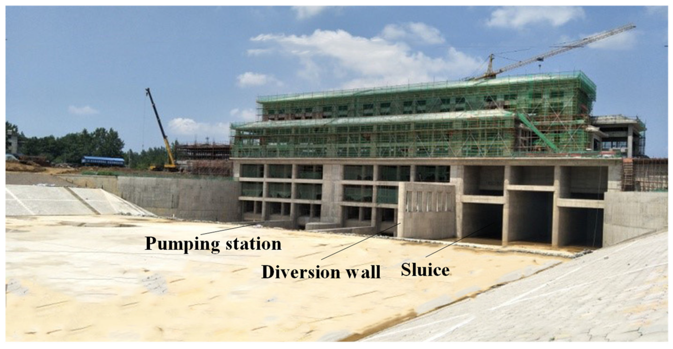
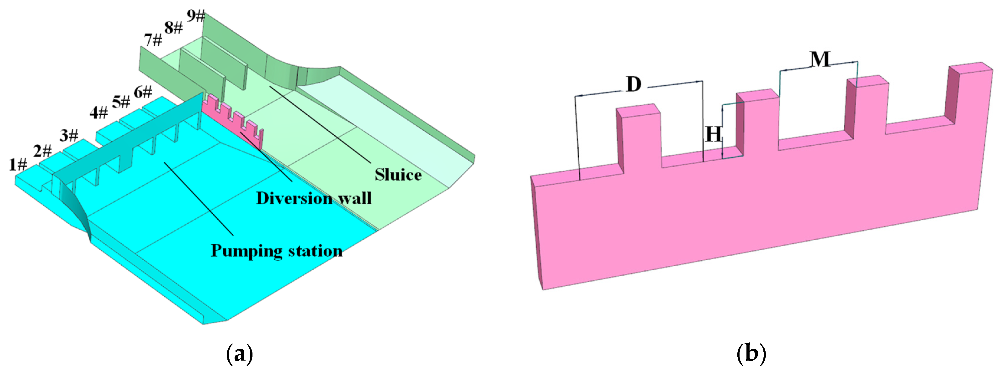
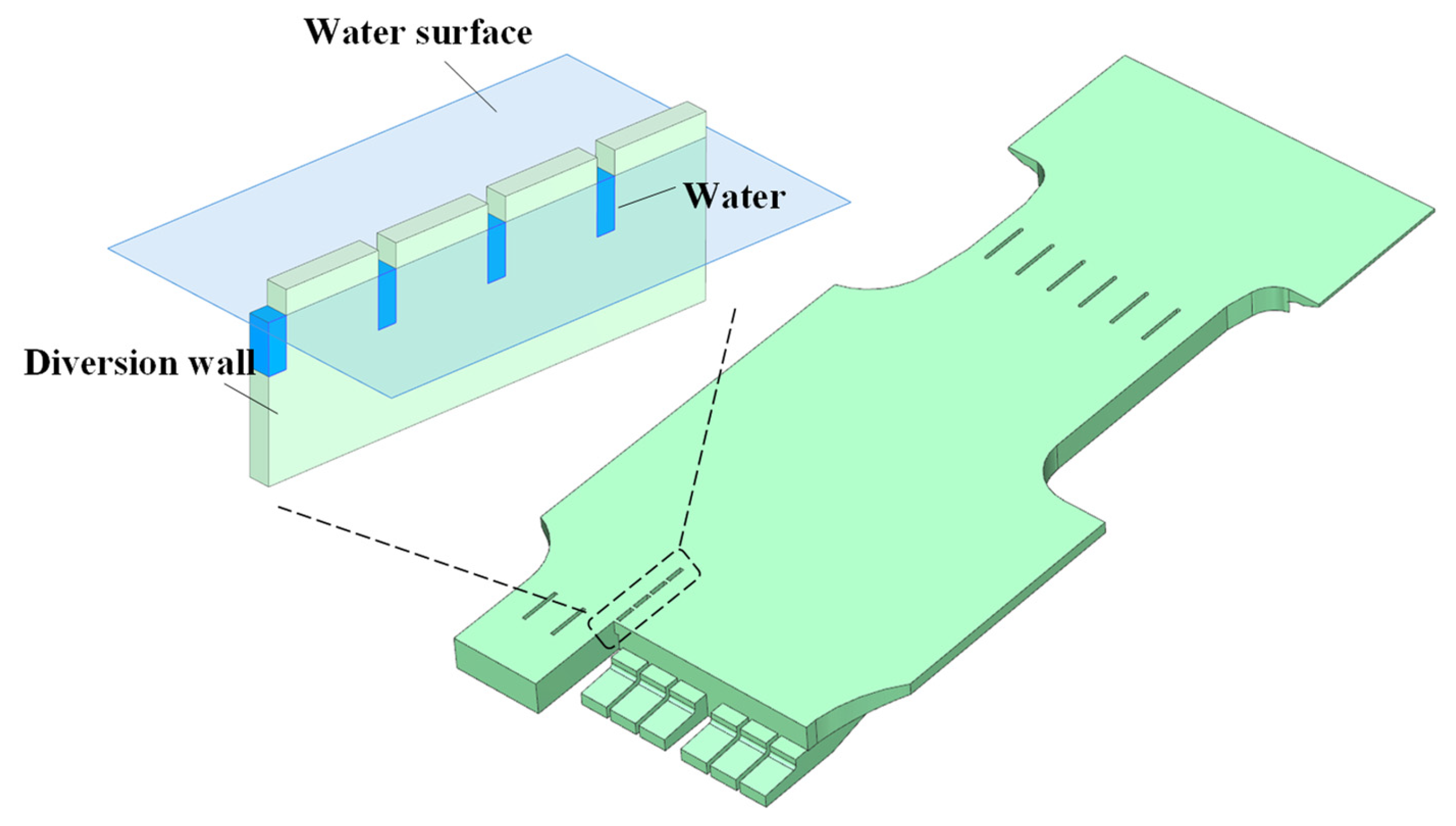
2.1. Study Subjects and Factors

As shown in Figure 1, the object of this study was the perforated diversion wall of a combined sluice-pumping station. The studied combined sluice-pumping station consisted of a pumping station and a sluice, with six pump units set in the pumping station and the sluice consisting of three chambers. In Figure 2, the three-dimensional layout of the diversion wall is displayed along with the schematic diagram of the perforated diversion wall of the combined sluice-pumping station. Factors in the optimization study of the perforated diversion wall include hole width M, hole center distance D and hole depth H.

2.2. Evaluation Indicator Selection Method

For the combined sluice-pumping station project, the flow regime in the forebay can affect the efficiency of the pump unit and the safety of the pumping station as well as the operation of the sluice and the safety of navigable ships. The uniformity of axial velocity distribution and the maximum transverse velocity are essential indicators that properly reflect the quality of flow pattern [24]. However, it is necessary to further determine which location of the above parameters should be selected as the optimization evaluation index through model experiments and numerical simulations.

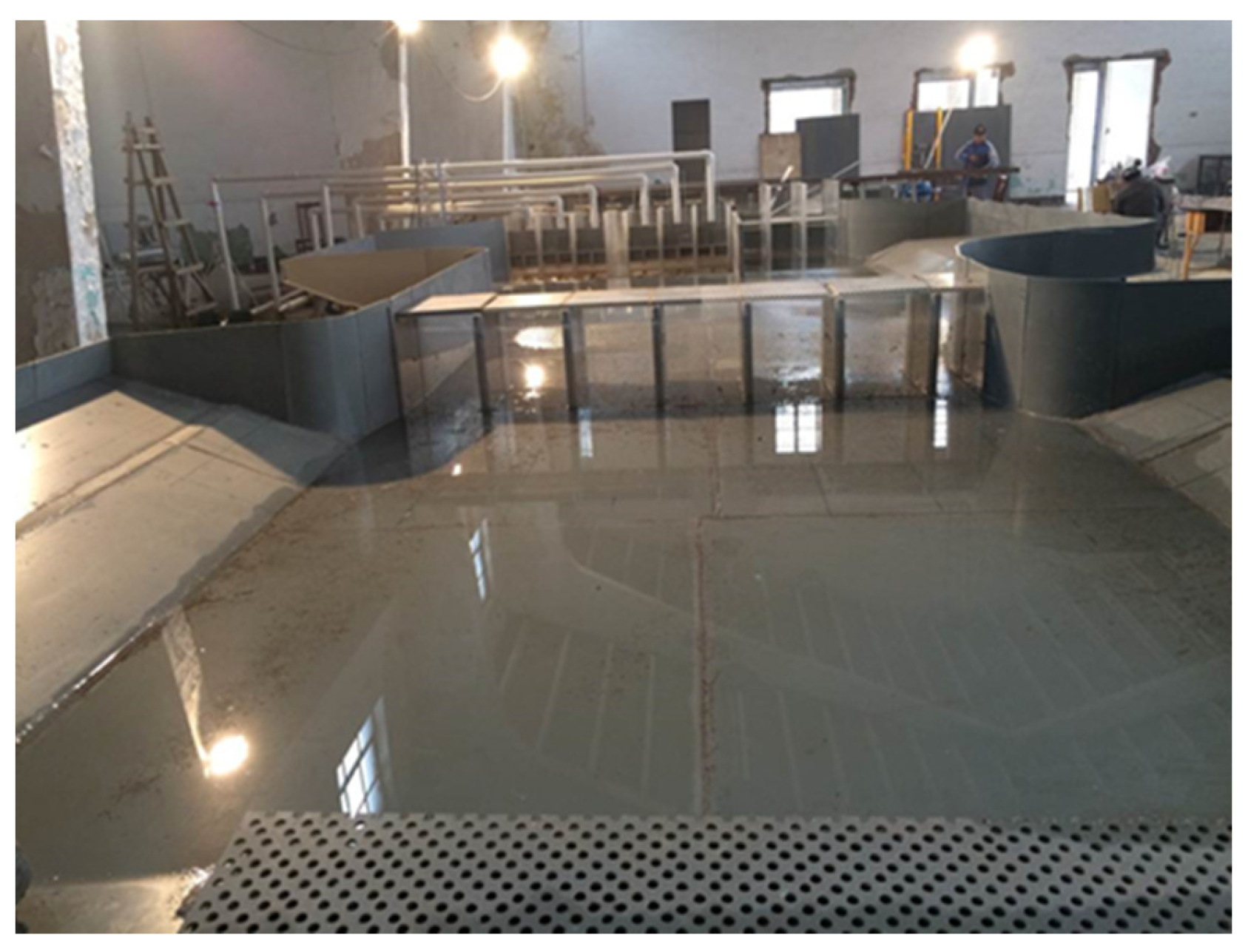
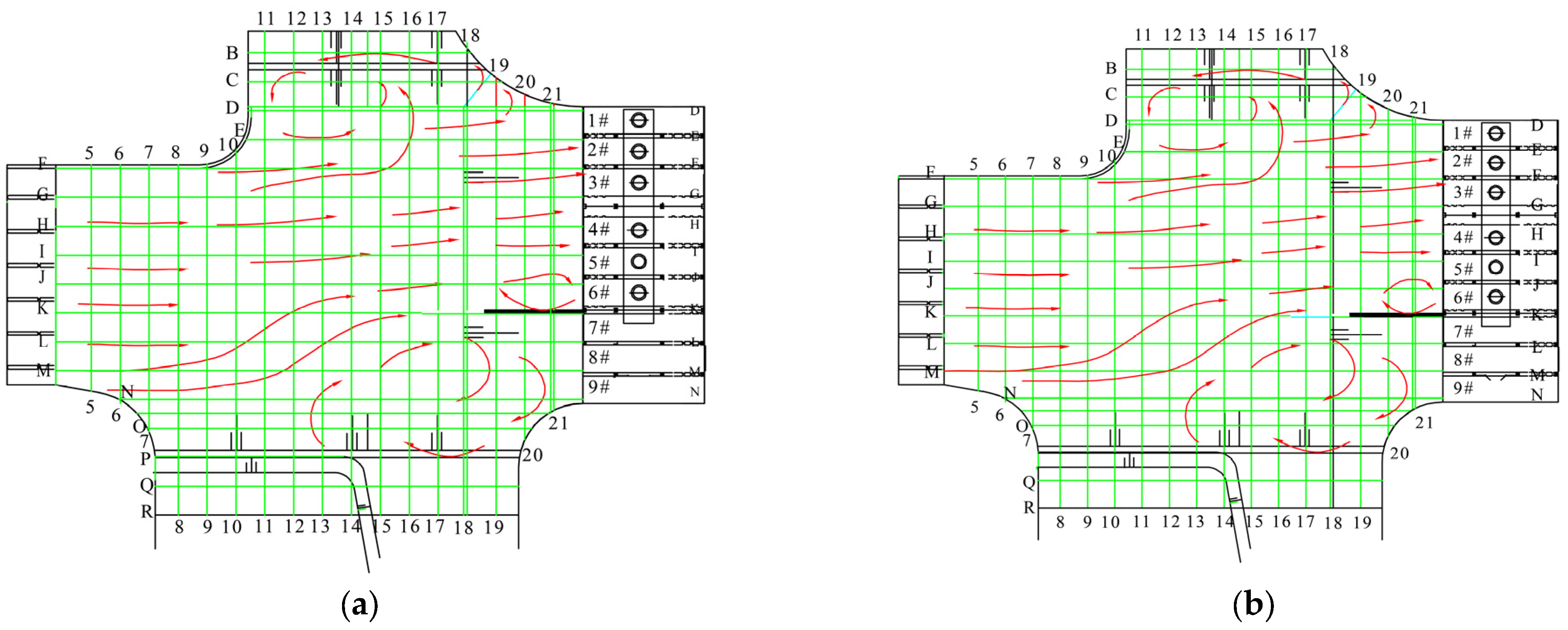
2.2.1. Physical Model Experiments

Taking the aforementioned combined sluice-pumping station as an example, the layout of the model test and the overall site diagram of the model are shown in Figure 3 and Figure 4 [24]. The scope of the model experiment study was from the end of the upstream slope protection to the downstream apron section, including the downstream channel with a total length of about 500 m and, the width was about 192 m from the upstream wing wall of flood drainage and sewage maintenance sluice to the downstream slope protection of the pumping station exit control sluice. The pump inlet channels were numbered as 1#, 2#, 3#, 4#, 5# and 6#. The 1# inlet channel was positioned in close proximity to the left wing wall of the approach river, while the 6# inlet channel was located closer to the sluice. The forebay and river bottom plate were situated at an elevation of 13.4 m, whereas the inlet pool bottom plate was located at an elevation of 6.65 m. The sluice was designed with three sluice chambers, numbered 7#, 8# and 9#, among which sluice chamber 7# was close to the pumping station side and sluice chamber 9# was positioned closer to the right wing wall of the approach river. The elevation of the sluice floor was 11.4 m. The sluice and the pumping station were separated by a diversion wall with its length of 25 m, width of 1.2 m and height of 8.8 m. The primary purpose of the project was to control and manage floodwaters and drainage, which was accomplished through two operational modes: self-draining (facilitated by the use of sluices) and pumping (provided by the pumping station). During operation of the pumping station, the sluice gate remains closed with upstream and downstream water levels designed to be 21 m and 24.3 m, respectively. However, upon opening the sluice gate, the pumping station ceased operation, causing the upstream water level to rise to 22.2 m, while the downstream water level decreased to 22.05 m. The model geometric scale λ_l was 30.

(1)

Investigation of the flow regime in the forebay during pump operation in the original design scheme.

The scheme was carried out under the condition of pumping, in which all pump units ran and the sluice was closed. The corresponding flow Q was 180 m³/s (model flow Q_m was 131.45 m³/h) and the water level of the upper stream h_s was 21 m (model water depth was 25.3 cm) and the lower stream h_x was 24.3 m (model water depth was 36.3 cm).

Figure 5 displays the flow patterns of the surface layer and the bottom layer under pumping conditions. It is evident from the figure that the flow patterns of the bottom layer and the surface layer in the forebay are highly comparable. The water flowed into the forebay of the pumping station from the direction of the sluice. Under the condition of pumping, the counterclockwise vortex flow appeared in the forebay, which is mainly located on the left side of the diversion wall and the left bank. Since the vortex zone of the left bank is far from the inlet channel, it is no longer considered in this paper. The vortex zone on the left of the diversion wall began to appear at cross-section 19-19 and continued to the front of inlet channel 6#. Thus, a cavitation phenomenon may be produced in the pump, causing pump vibration and even threatening the stable operation of the pump.

(2)

Investigation of the flow regime in the forebay during sluice operation in the original design scheme.

The scheme was carried out under the condition of self-draining, in which three sluices were opened and the pump units were all closed. The corresponding flow Q was 412 m³/s (model flow Q_m was 300.88 m³/h), the water level of the upstream h_s was 22.2 m (model water depth was 29.3 cm) and the downstream h_x was 22.05 m (model water depth was 28.8 cm).

Figure 6 displays flow pattern diagrams for the surface layer and bottom layer under self-draining conditions. The bottom layer flow pattern in the forebay was found to be consistent with that of the surface layer. Specifically, a pronounced diagonal flow was observed in front of the diversion wall, while a roundabout region appeared near the right side of the wall in front of the sluice along the flow channel of the pumping station.

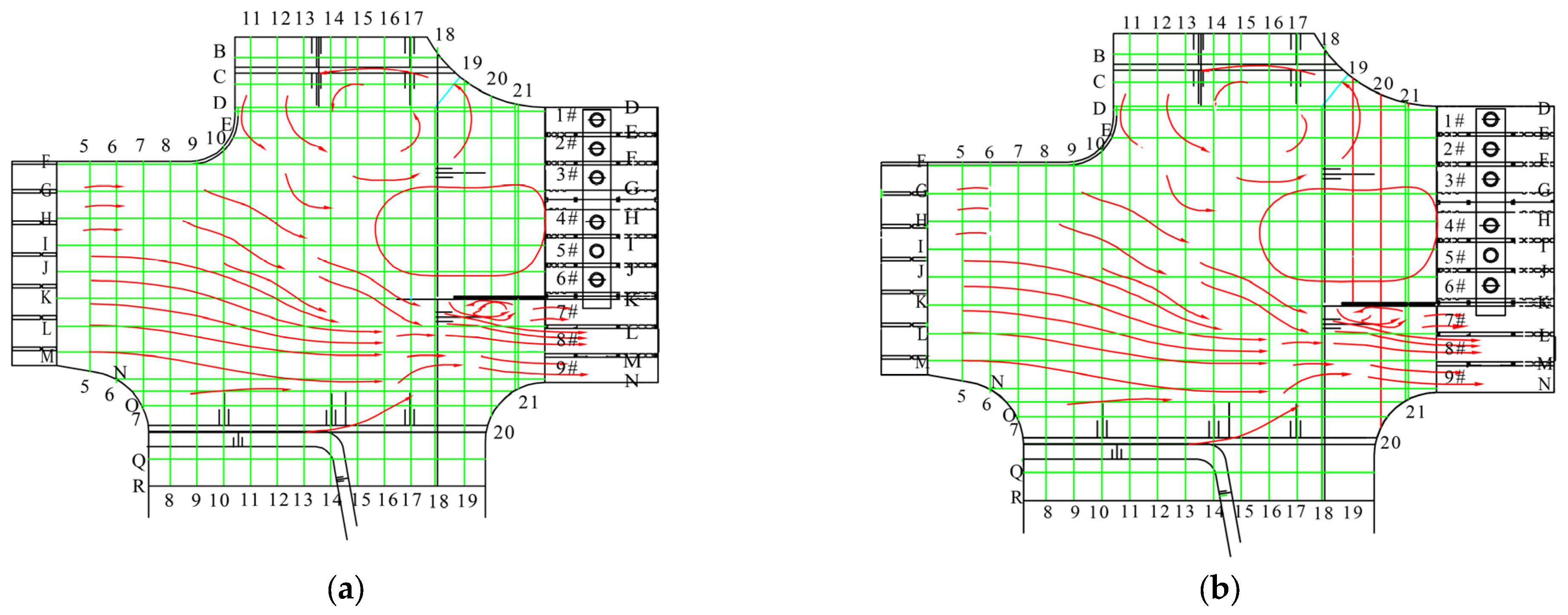
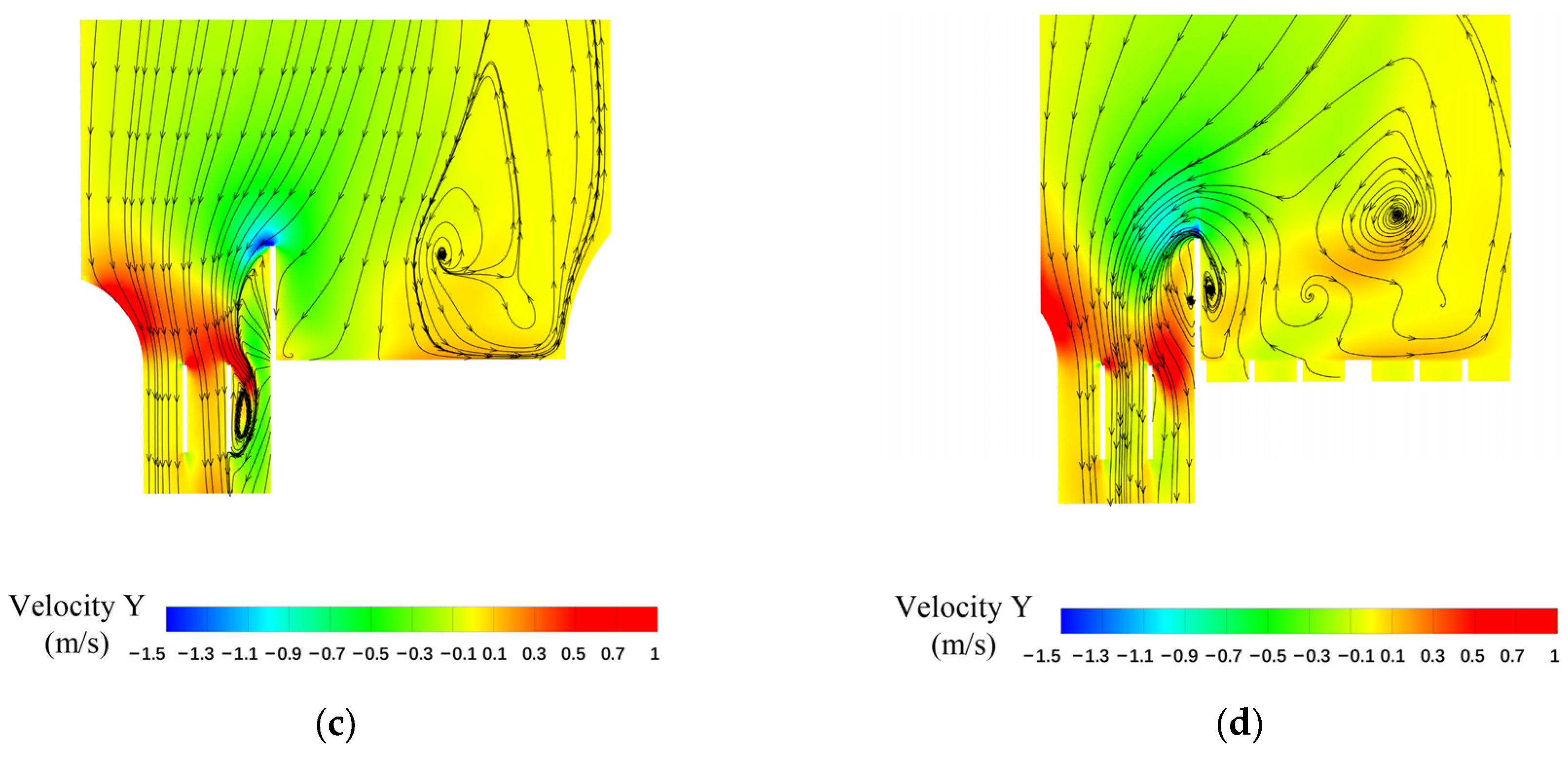
2.2.2. Numerical Simulation Analysis

In order to compare with the results of physical model experiments and facilitate further research, a computational fluid dynamics (CFD) model of the combined sluice-pumping station was developed to simulate inflow patterns. Using the RNG k–ε vorticity viscosity model and Reynolds Averaged Navier–Stokes Equations (RANS), a model that has been proven to be effective at handling complex curved streamlines was constructed [25]. The Fluent software’s built-in finite volume method solver was utilized, and the SIMPLEC algorithm was applied to iteratively solve the discrete equations in the model domain until convergence was achieved.

(1)

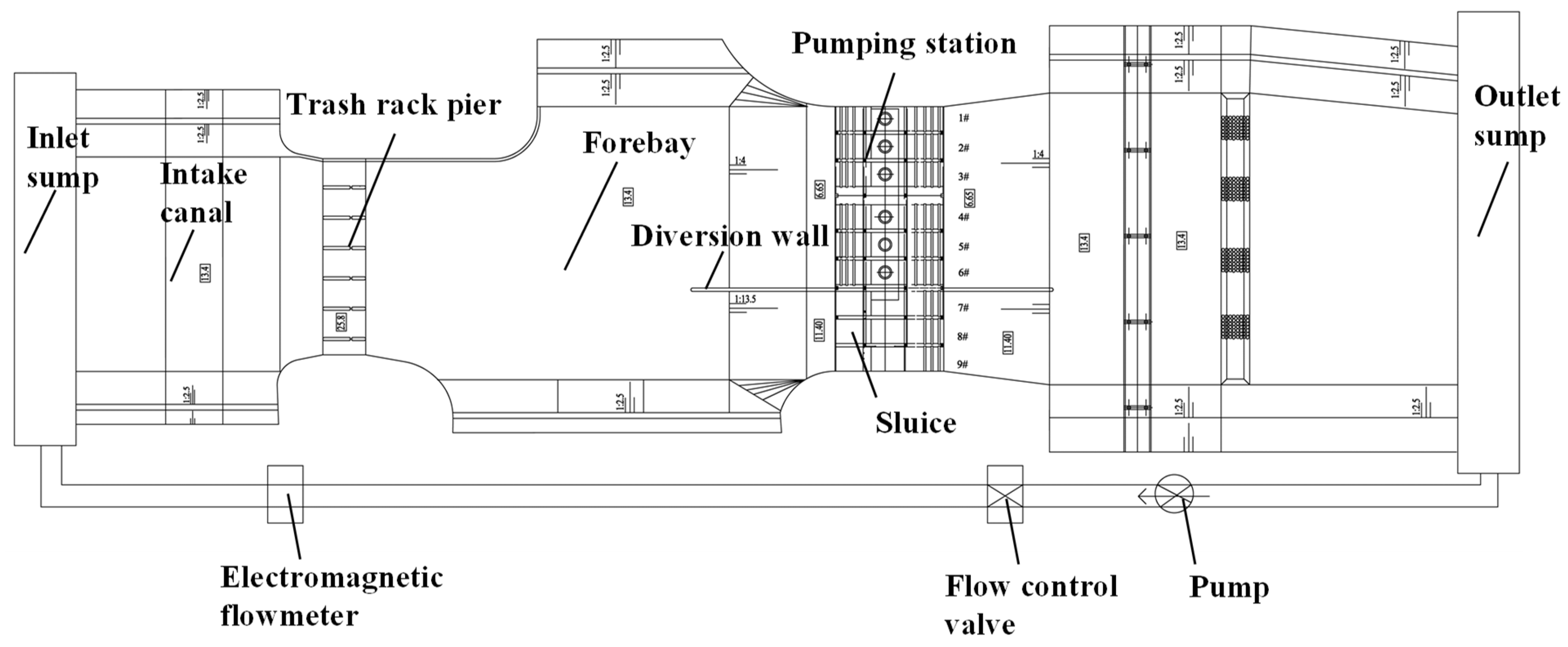
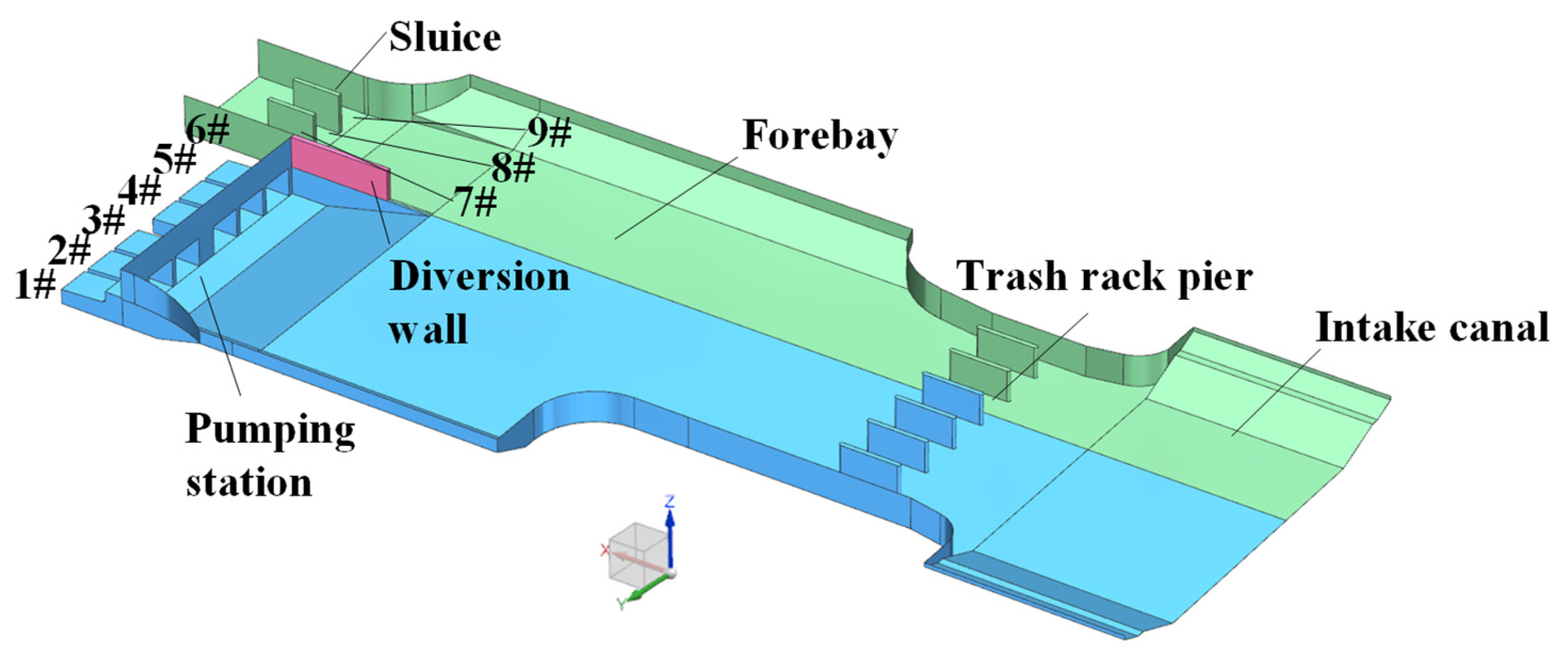
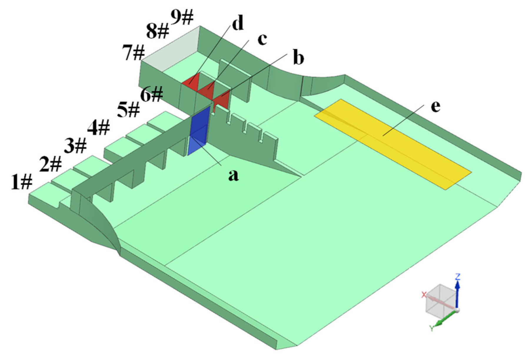
Modeling range

In Figure 7, a 3D model of the abovementioned combined sluice-pumping station is displayed, and this model is a typical asymmetric combined sluice-pumping station layout. In order to ensure the precision of the numerical simulation study and reduce the influence of missing upstream and downstream structures on the flow pattern simulation, the inlet channel was extended, and the modeling scope was consistent for each calculation scheme. The key parameters studied in this paper were the hole size of the diversion wall, including hole width M, hole spacing D and hole depth H, which are shown in Figure 2b.

(2)

Meshing

The computational model domain was relatively complex, and the application of tetrahedral unstructured mesh could improve the efficiency of cell division. The meshing quality is controlled by the aspect ratio, skewness and orthogonal quality, and the cell independence analysis showed that when the number of cells was greater than 1.6 × 10⁶, there was no significant difference in the calculation results, so the number of control cells was greater than 1.6 × 10⁶.

(3)

Boundary condition

Four boundary conditions were adopted in each calculation model. The first type of boundary condition was velocity inlet [26]. Both under the condition of self-draining and pumping, the inlet boundary was defined at the inlet of the intake canal. Under the condition of pumping, the inlet velocity was 0.27 m/s, and under the condition of self-draining, the inlet velocity was 0.52 m/s. The second type of boundary condition was free outflow that is under the pumping condition. The six inlet channels 1#~6# were appropriately extended as the outlet boundary to meet the condition that turbulence was fully developed. The six pump units were of the same model, so the flow weight of the six outlets were all set as 1. Similarly, under the condition of self-draining, the length of the sluice chamber should be extended appropriately, and the outlet boundary was set at the end of the sluice. The third type of boundary condition was set on the water surface. Because the water surface changes little with time, the shear stress effect of air on the water surface was ignored and the “rigid cover assumption” was selected for calculation. In other words, the water surface was set as symmetry [3,27,28]. In addition to the aforementioned boundary conditions, the last condition was the non-slip standard wall, which was adopted in all other walls.

(4)

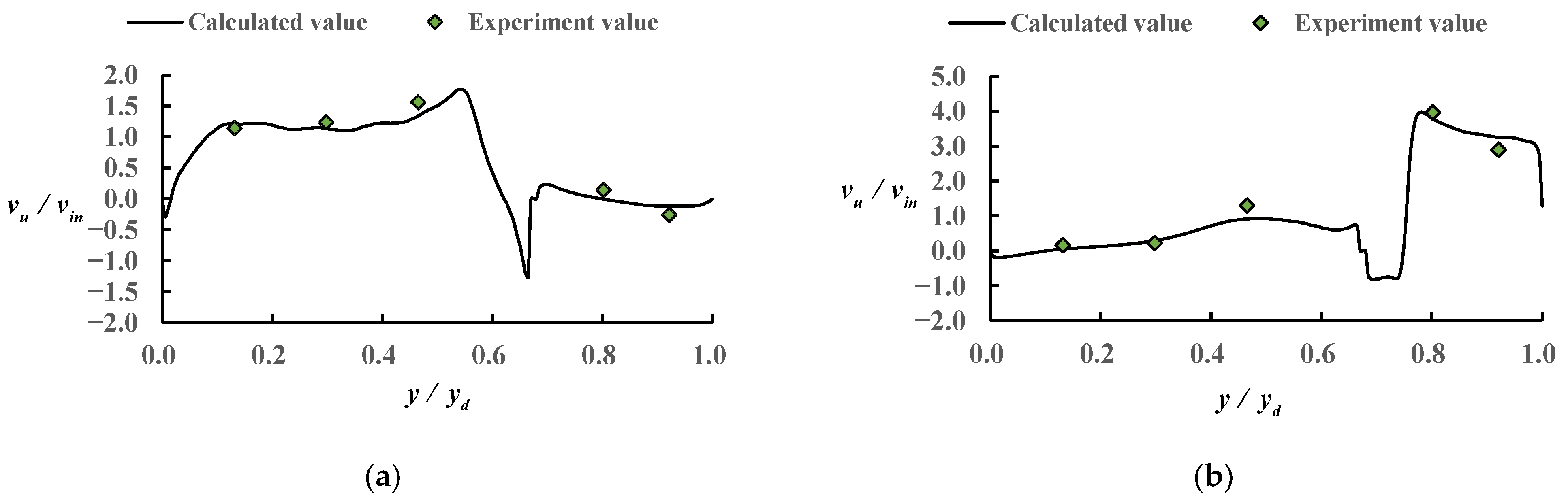
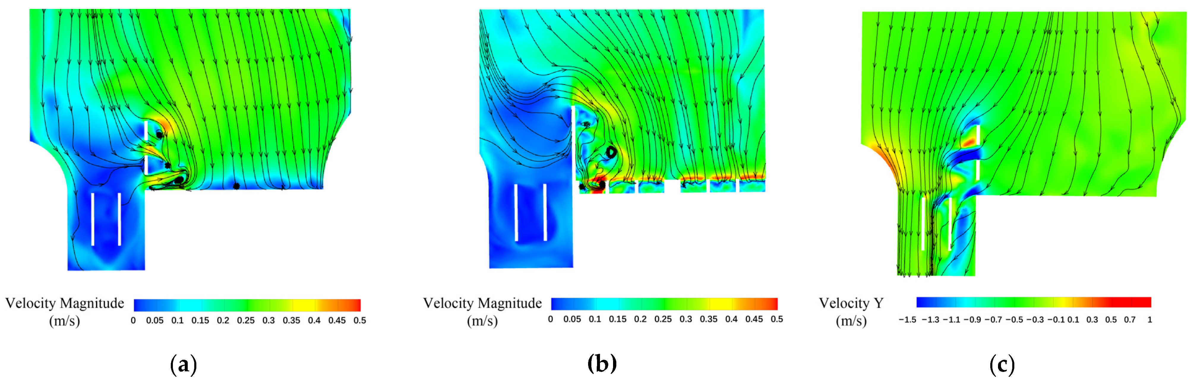
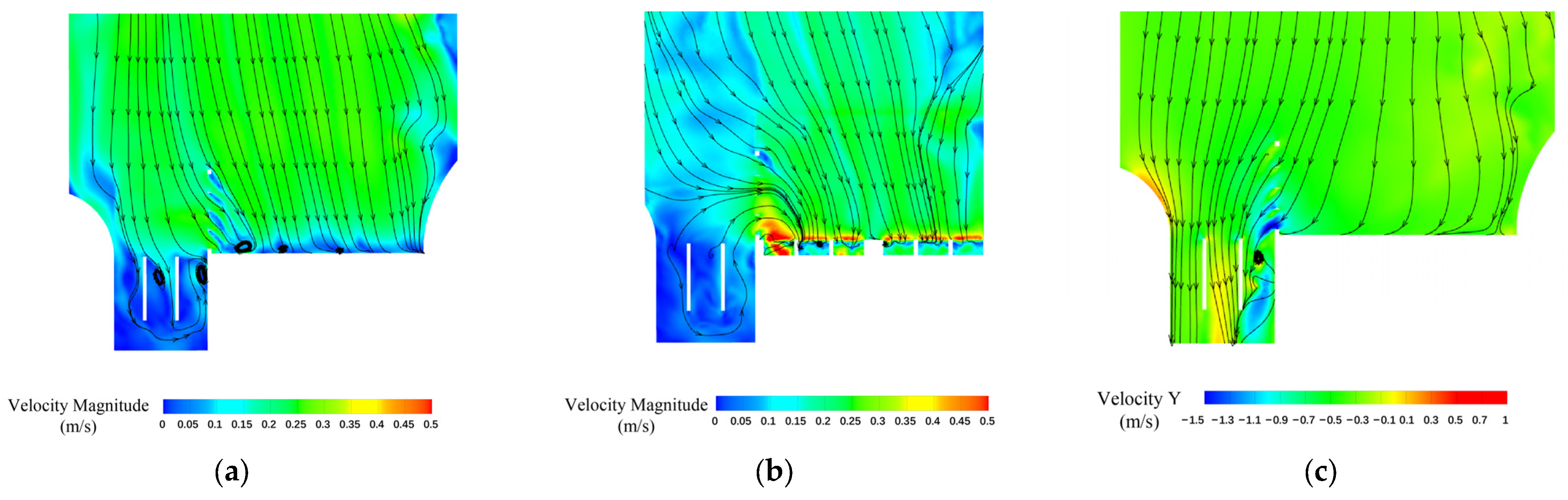
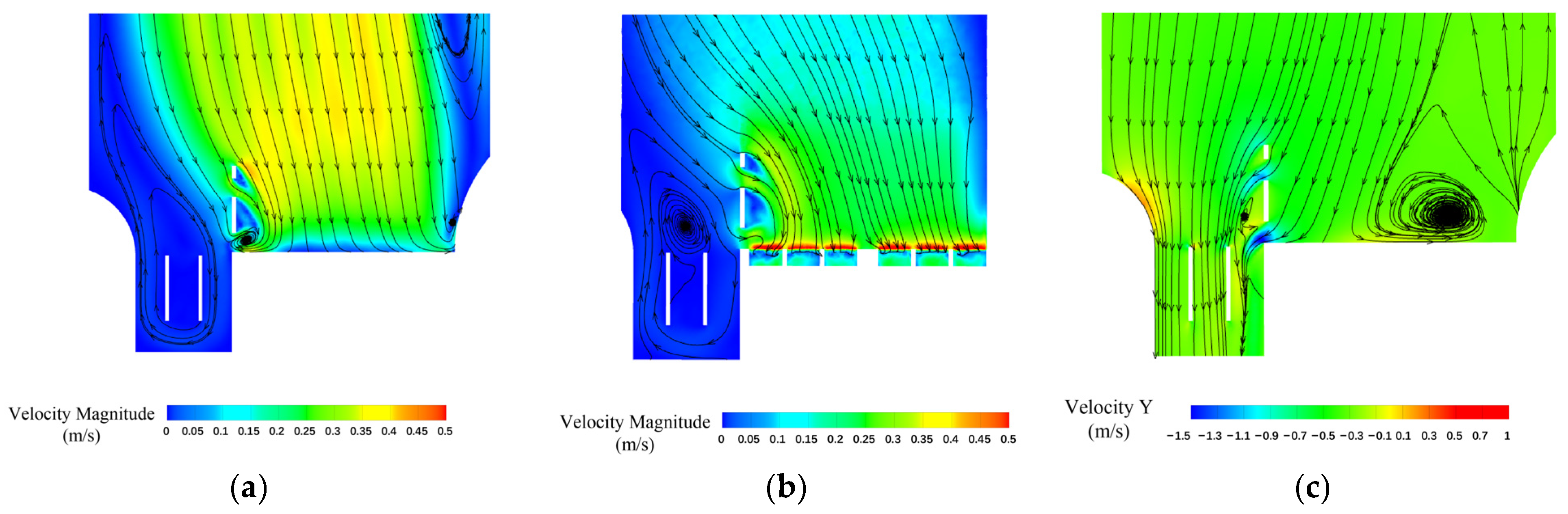
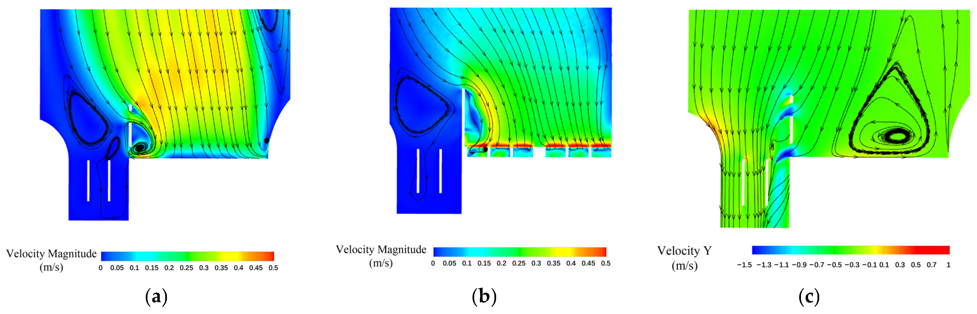
Comparison of Simulation Results

Figure 8 presents the distribution of surface layer velocities in the 20-20 cross-section as shown in Figure 6. To facilitate comparison, the x-direction velocity (v_u) at each point on the surface layer of the 20-20 cross-section was normalized by dividing it by the average inlet velocity (v_in) of the intake channel, which achieves a dimensionless velocity and is used as the y-axis. The x-axis represents the distance (y) in meters from the left wing wall of the forebay to the velocity measurement point relative to the width (y_d) of the 20-20 cross-section. The left wing wall is located at y/y_d = 0, and the right lateral wall is at an x-coordinate of 1.

Figure 9 shows the numerical simulation results of the diversion wall without a hole in the original scheme. The aforementioned results are consistent with the findings reported in the literature [20], which were based on numerical simulations. Under pumping conditions, the adverse flow pattern in the forebay primarily affected inlet channel 6#, leading to a deteriorating inflow condition that posed a threat to the stable operation of the pumping unit. In contrast, under self-draining conditions, the flow pattern in front of sluice chamber 7# exhibited a high level of disorder, which resulted in a reduction of the sluice’s flow capacity. Therefore, the uniformity of the axial velocity distribution of inlet channel 6# was selected as the evaluation indicator for pumping conditions, while the uniformity of the axial velocity distribution of sluice chamber 7# was chosen as the evaluation indicator for self-draining conditions. Additionally, to meet the navigation requirement under self-draining conditions, the evaluation indicator included the transverse velocity ahead of the operating sluice [29].

3. Optimization Method of Hole Parameters of Diversion Wall Based on Numerical Simulation

3.1. Obtaining Results from Numerical Simulation

In this study, CFD-Post was applied for post-processing and data reading, and the monitoring section of post-processing data is shown in Figure 10. According to the analysis in Section 2.2, under the condition of pumping, the flow pattern at the inlet side of inlet channel 6# was poor, which had a greater impact on the normal operation of the pump unit. Therefore, the calculation and monitoring section was arranged at 0.5 m in front of inlet channel #6. Under the condition of self-draining, the flow pattern of sluice chamber 7# was poor, so monitoring sections b, c and d were arranged in sluice chamber 7#. In addition, under the condition of self-draining, the sluice tends to be used to realize navigation functions, in which case monitoring section e is set in the navigation channel area [29].

In this study, the uniformity of axial velocity distribution and the maximum transverse velocity were adopted to evaluate the flow pattern of the forebay. The uniformity of axial velocity distribution and the maximum transverse velocity can be calculated by Equations (1) and (2).

$${\lambda }_i=\{1-\frac{1}{\overline{V_a}}\sqrt{{\displaystyle \sum _{i=1}^n{(V_{ai}-\overline{V_a})}^2/n}}\}\times 100\%$$

(1)

$$V_{yi}=\max \left\{v_{yi}{}_1,v_y{}_{i2}\cdots v_{yij}\cdots v_{yin}\right\}$$

(2)

In Equations (1) and (2), λ_i is the uniformity of axial velocity distribution of monitoring section i; $\overline{V_a}$ is the average axial velocity on monitoring plane i; $V_{ai}$ is the axial velocity of the calculation unit on the monitoring plane i; n is the number of calculation units of monitoring section i; $V_{yi}$ is the maximum transverse velocity on monitoring section i and $v_{yij}$ is the value of transverse velocity on the element plane j of monitoring plane i.

Equations (3)–(5) were used to calculate the evaluation indicator of the diversion wall hole parameters under both self-draining and pumping conditions.

Pumping condition:

$$y_1={\lambda }_a$$

(3)

Self-draining condition:

$$y_2=\left({\lambda }_b+{\lambda }_c+{\lambda }_d\right)/3$$

(4)

$$y_3=V_{ye}$$

(5)

where y₁ is the indicator evaluating the flow pattern of the combined sluice-pumping station under the pumping condition, and y₂ and y₃ are the indicators evaluating the flow pattern under the self-draining condition.

3.2. Design of Hole Parameters of Diversion Wall Based on Orthogonal Test

In this study, the parameters of the perforated diversion wall of the orthogonal test were hole width M, center distance of adjacent hole D and hole depth H. The above three factors were selected in the orthogonal design of hole parameters, and five levels were selected for each factor. The parameters corresponding to each level of the factor are listed in

Table 1. Orthogonal design table of hole parameters of diversion wall.

Level	Factor
	M/m	D/m	H/m
1	1.0	5.6	2.0
2	2.1	6.25	3.7
3	3.2	8.33	5.4
4	4.3	12.5	7.1
5	5.4	25	8.8

.

According to the selected factors and level number, orthogonal table L25(5⁴) was selected for orthogonal design in both conditions.

After conducting orthogonal testing, we performed a range and main effect analysis to determine the influence of different factors on improving the flow pattern in both the sluice and inlet channel. As a result, we could obtain optimized combinations of geometric parameters for the holes under two different working conditions.

3.3. Establishment of Comprehensive Evaluation Indicator Based on Coefficient of Variation Method

Three evaluation indicators were used: y₁ reflects the flow pattern under pumping conditions, and y₂ and y₃ reflect the flow pattern under self-draining conditions. In this paper, the aforementioned evaluation indexes were combined, given different weights and condensed into a comprehensive indicator, thus simplifying the problem [30]. To determine the weight coefficient, the coefficient of variation method [31,32] was adopted in this paper, and the specific steps of each index are listed as follows:

(1)

Assuming the evaluation system contains K indicators, that is $y_k$ (k = 1, 2, 3…K) and each indicator contains n experimental data items $y_{kj}$ (k = 1, 2, 3…K, j = 1, 2, 3…n).

(2)

The value of the evaluation indicator is normalized to make the data of different units comparable. If the larger original series is better recognized, Equation (6) can be used for calculation. If the smaller original series is better recognized, Equation (7) can be used for calculation.

$$Y_{kj}=\frac{y_{kj}-\min (y_{kj},j=1,2,\cdots ,n)}{\max (y_{kj},j=1,2,\cdots ,n)-\min (y_{kj},j=1,2,\cdots ,n)}$$

(6)

$$Y_{kj}=\frac{\max (y_{kj},j=1,2,\cdots ,n)-y_{kj}}{\max (y_{kj},j=1,2,\cdots ,n)-\min (y_{kj},j=1,2,\cdots ,n)}$$

(7)

where $k=1, 2, 3\cdots , K$ and $j=1, 2, 3\dots , n$. K is the number of evaluation indicators, and n is the number of experimental data items. Y_kj ($j=1, 2, 3\dots , n$) is the experimental data items after normalization.

The normalized evaluation indicator is $Y_k$, $(k=1, 2, 3\cdots ,K)$.

(3)

Calculating standard deviation

$$\overline{Y_k}=\frac{1}{n}{\displaystyle \sum _{j=1}^n{Y}_{kj}}, k=1, 2, 3\cdots , K$$

(8)

$$ST{D}_k=\sqrt{\frac{1}{n}{\displaystyle \sum _{j=1}^n\left(Y_{kj}-\overline{Y_k}\right)}}, k=1, 2, 3\cdots , K$$

(9)

(4)

Calculating the coefficient of variation of each indicator

$$C{V}_k=\raisebox{1ex}{$ST{D}_k$}\!\left/ \!\raisebox{-1ex}{$\overline{Y_k}$}\right., k=1, 2, 3\cdots , K$$

(10)

(5)

The weight coefficient of each indicator was obtained by the normalization of V_k

$$W_k=\raisebox{1ex}{$C{V}_k$}\!\left/ \!\raisebox{-1ex}{${\displaystyle \sum _k^{K}C{V}_k}$}\right.$$

(11)

(6)

The final:

$$Y=W_1{Y}_1+W_2{Y}_2+W_3{Y}_3$$

(12)

In Equations (8)–(12), $k=1, 2, 3\cdots , K$ and $j=1, 2, 3\dots , n$. K is the number of evaluation indicators, and n is the number of experimental data items. Y_kj ($j=1, 2, 3\dots , n$) is the evaluation index after normalization, and $\overline{Y_k}$ is the average $Y_{kj}$ ($j=1, 2, 3\dots , n$) of n experimental data items. $ST{D}_k$, $C{V}_k$ and $W_k$ are the standard deviation, coefficient of variation and weight coefficient of indicator $Y_k$, respectively. $Y$ is the comprehensive evaluation indicator.

3.4. Establishment of Response Surface Model of Diversion Wall Hole Parameters

According to the orthogonal test scheme in Table 1, a numerical simulation calculation was carried out to obtain the hydraulic characteristics of the forebay under each scheme. A response surface model was established between Y₁, Y₂, Y₃ and M, D, H, respectively. Taking the comprehensive evaluation indicator Y as the objective function, the response surface model was established among the hole width M, the open hole center distance D and the open hole depth H. Equation (13) is the general form of the second-order response surface model.

$$y={\beta }_0+{\displaystyle \sum _{i=1}^k{\beta }_i{x}_i}+{\displaystyle \sum {\displaystyle \sum _{i<j}{\beta }_{ij}{x}_i{x}_j}}+{\displaystyle \sum _{i=1}^k{\beta }_{ii}{x}_i{}^2}+\epsilon$$

(13)

In Equation (13), ${\beta }_i$ represents the undetermined coefficients of the response surface, k is the number of independent variables, $\epsilon$ is residual, x_i are the input parameters and y is the response value.

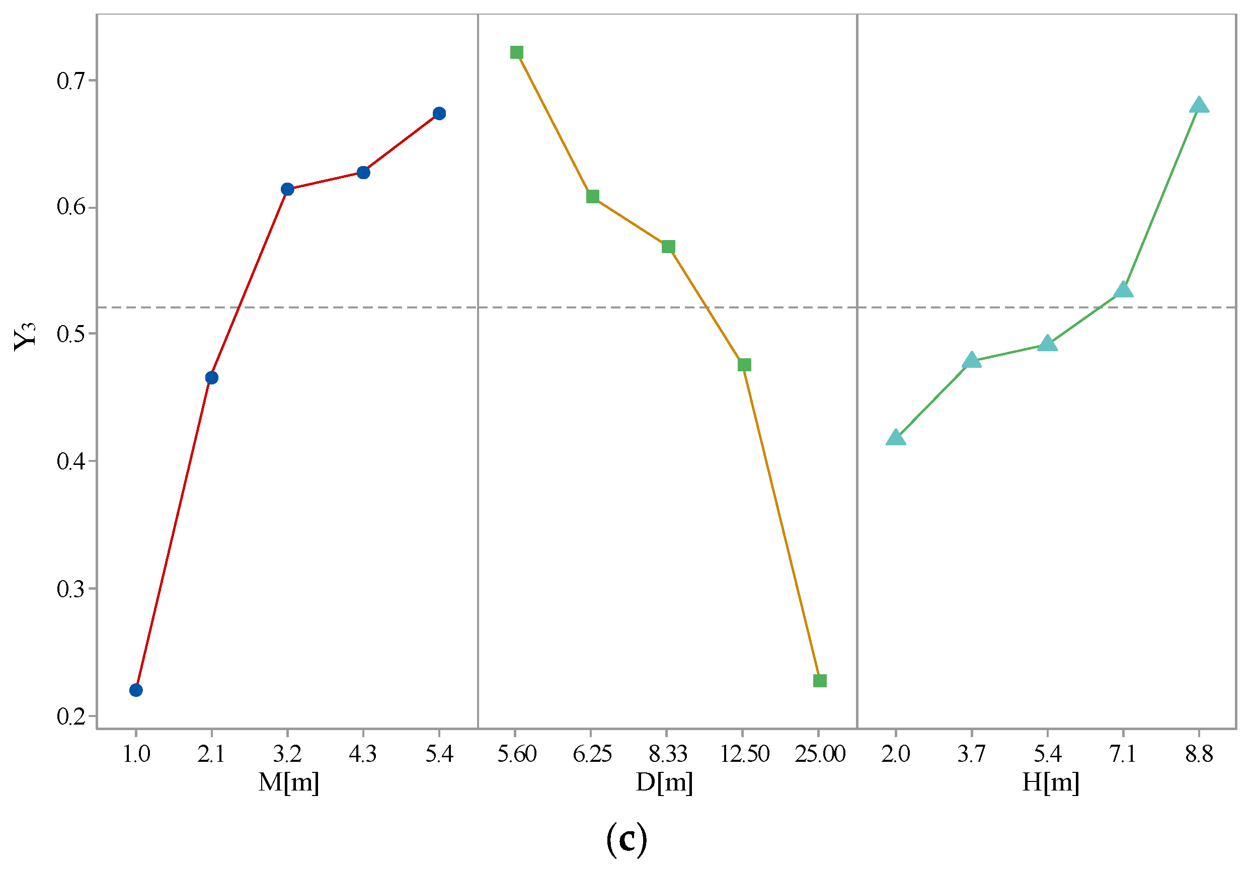
3.5. Analysis of Factors Influencing Objective Function

According to the response surface model between the diversion wall hole parameters and the four objective functions, the three-dimensional surface cloud map and response contour cloud map could be drawn between the hole width M, the hole center distance D and the hole depth H and Y₁, Y₂, Y₃ and the comprehensive evaluation indicator Y, which are the four evaluation indicators. According to the three-dimensional curved surface nephogram and response contour nephogram, the response of the diversion wall hole parameters to the four objective functions and the coupling effects on the objective functions can be analyzed.

3.6. Optimization Method of Hole Parameters

The mathematical model of multi-objective optimization of diversion wall hole parameters is:

$$\left\{\begin{array}{l}\max \lambda (M,D,H)\\ \min V_y(M,D,H)\end{array}\right.\left\{\begin{array}{l}{M}_{\min }\le M\le M_{\max }\\ D_{\min }\le D\le D_{\max }\\ H_{\min }\le H\le H_{\max }\end{array}\right.$$

(14)

In Equation (14), $\lambda$ is the uniformity of axial velocity distribution, $V_y$ is the maximum transverse velocity, M is the hole width, D is the hole center distance and H is the hole depth.

In this paper, M, D and H were taken as the independent variables of optimal design and Y₁, Y₂, Y₃ and Y were taken as the targets. The maximum value of four objective functions in the calculation area was solved by applying the fastest rising method. The gradient of the objective function Y₁, Y₂, Y₃ and Y at a certain point indicates that the function value rises fastest here, and this is used to search the maximum value of the function in a certain area [31]. Through calculation, the hole parameters corresponding to the maximum value of each objective function were obtained; that is, the optimal scheme can be required by each objective function. Then, the optimized schemes obtained were numerically simulated by Fluent, and the indexes y₁, y₂ and y₃ were analyzed so that parameters M, D and H could be finally optimized.

According to the above analysis, the steps to optimize the hole parameters of the diversion wall are as follows:

(1)

The model test and numerical simulation were used to calculate and analyze the hydrodynamic characteristics of the forebay under the original design scheme of the combined sluice-pumping station, and the evaluation indicators of the optimization of the hole parameters of the diversion wall under the conditions of pumping and self-draining were obtained. The rationality and reliability of the numerical simulation method and the calculation model were verified.

(2)

Three factors, including hole width M, hole center distance D and hole depth H, were selected for the diversion wall, and five levels were selected for each factor to carry out the design of the orthogonal test scheme.

(3)

The software of UG and MESH were used to establish 50 different calculation models for the orthogonal experimental design scheme, and the Fluent software was used to calculate the water force characteristics of the forebay.

(4)

Through the range analysis of the numerical simulation results of the orthogonal test scheme, an optimized scheme of hole parameters of the diversion wall could be obtained.

(5)

According to the numerical simulation results, the weight coefficients of three evaluation indicators, namely Y₁, Y₂ and Y₃, were calculated, and the comprehensive evaluation indicator Y was established.

(6)

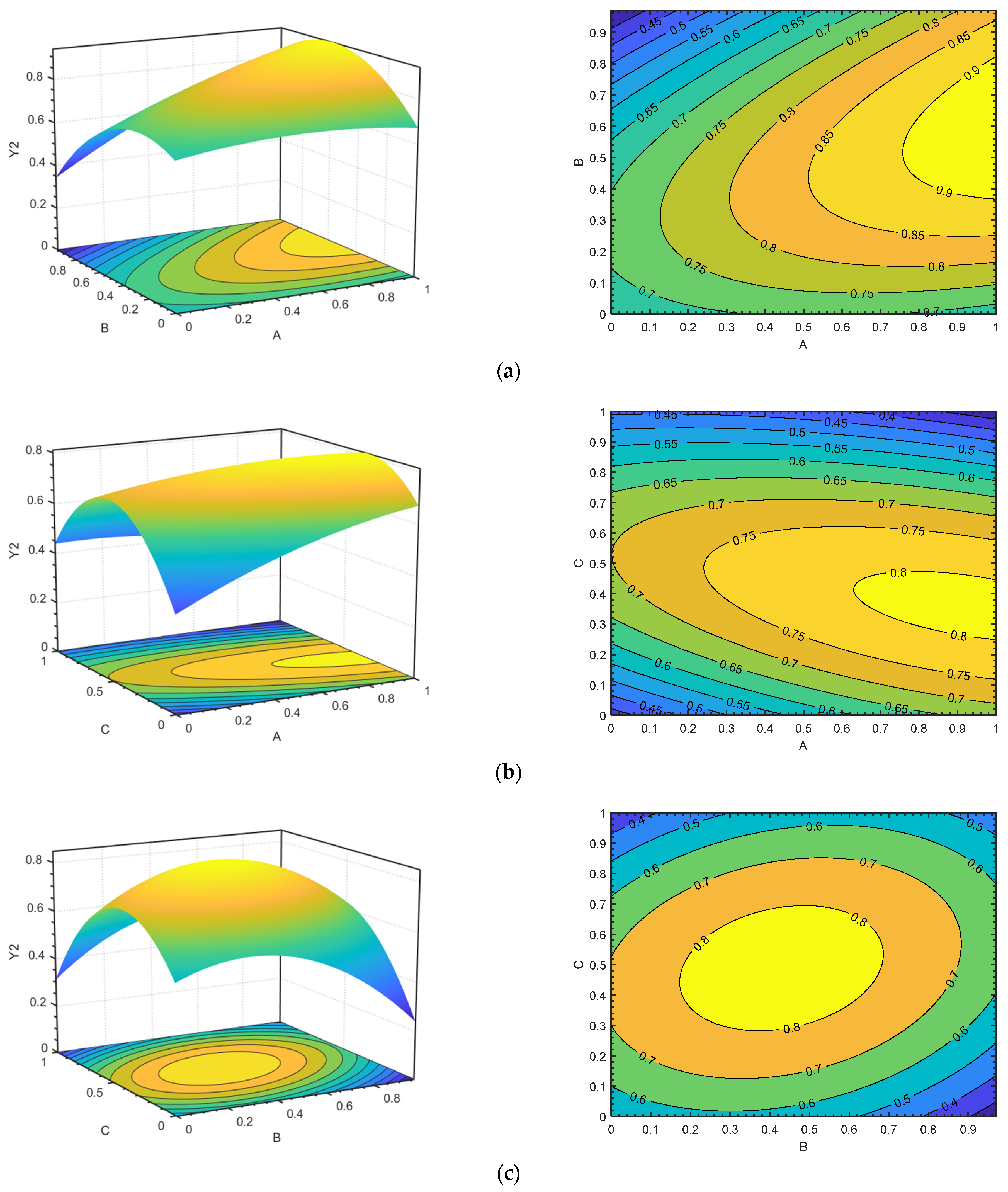
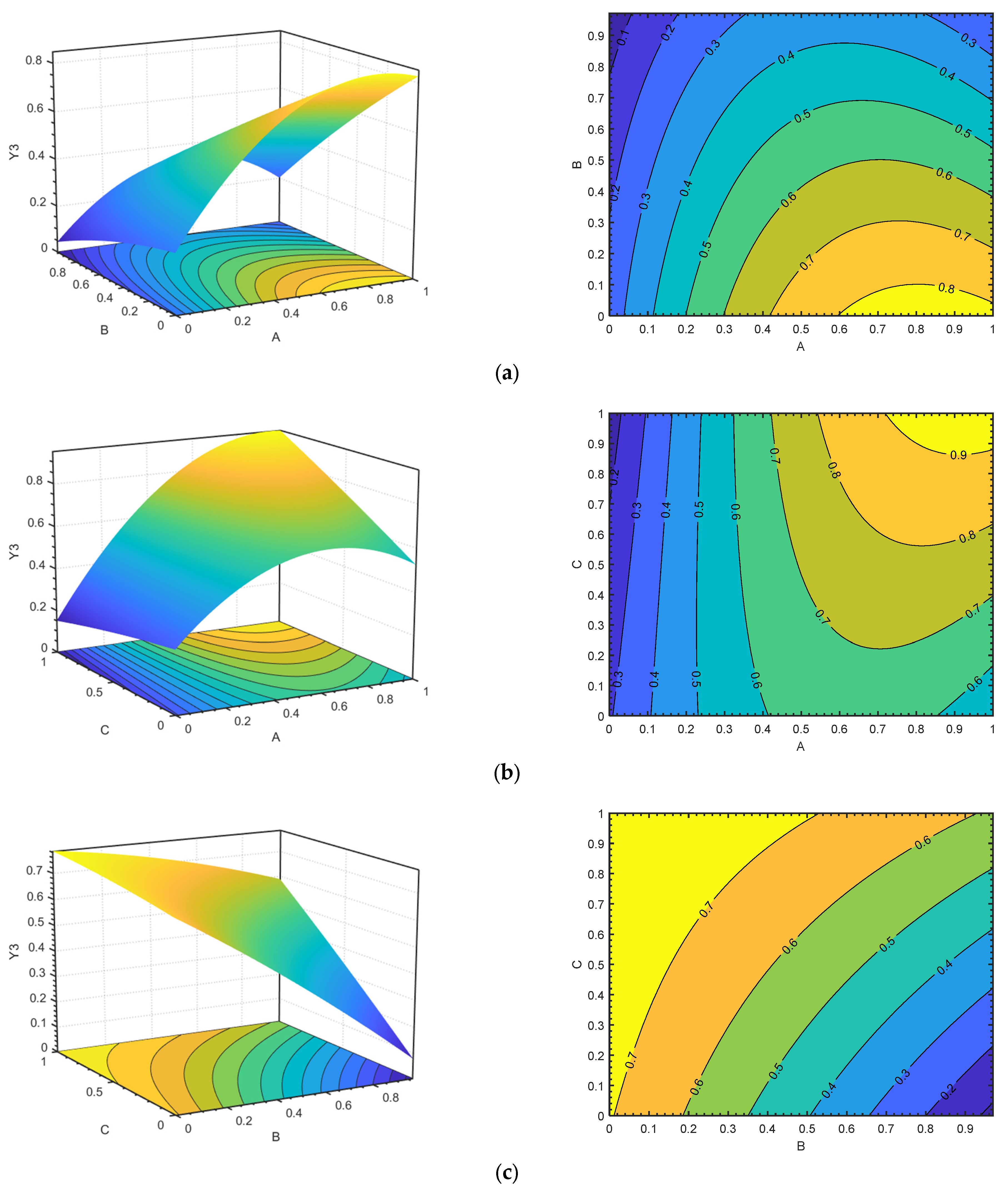
Y₁, Y₂, Y₃ and Y were taken as the objective functions, and the response surface models were established with M, D and H.

(7)

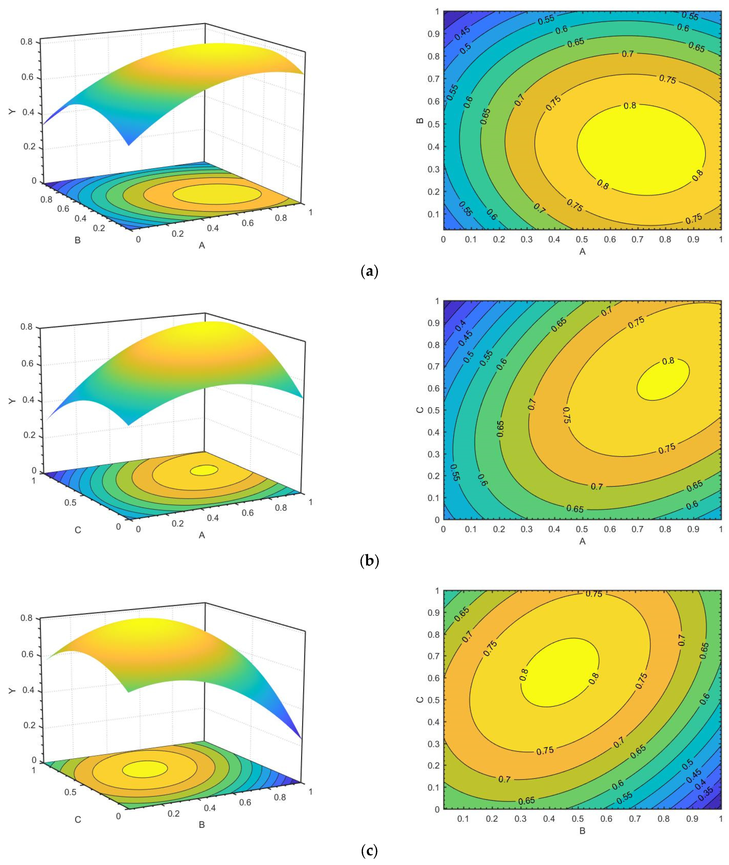
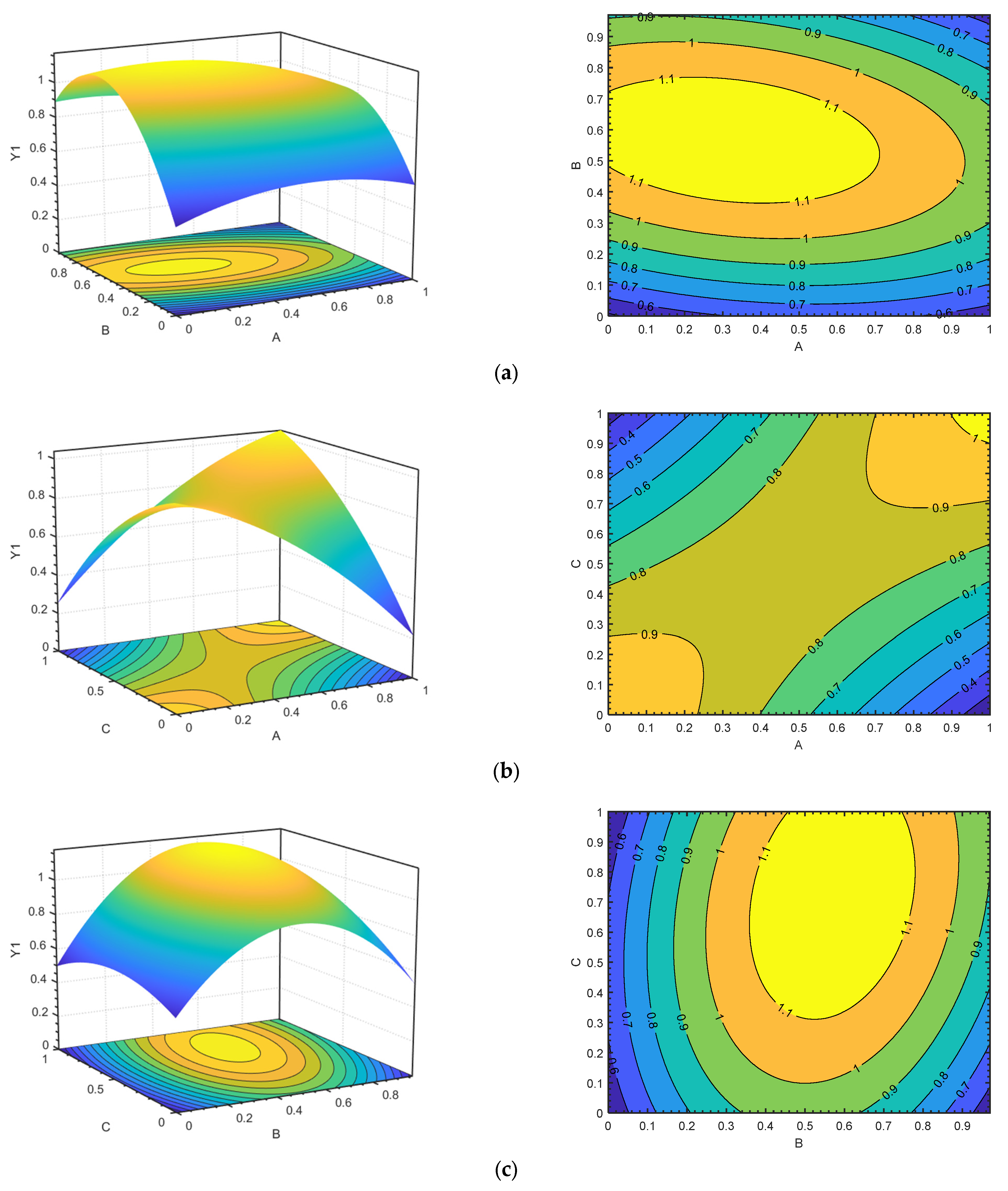
Three-dimensional response surface plot between the hole parameters and the objective function were drawn so that the principle of the influence of the hole parameters on the four objective functions could be analyzed and so the coupling relationship of hole parameters could be conducted.

(8)

The maximum values of the four objective functions Y₁, Y₂, Y₃ and Y in the calculation area were solved by the fastest rising method, and the corresponding orifice parameter schemes were obtained when the maximum values of each objective function were obtained.

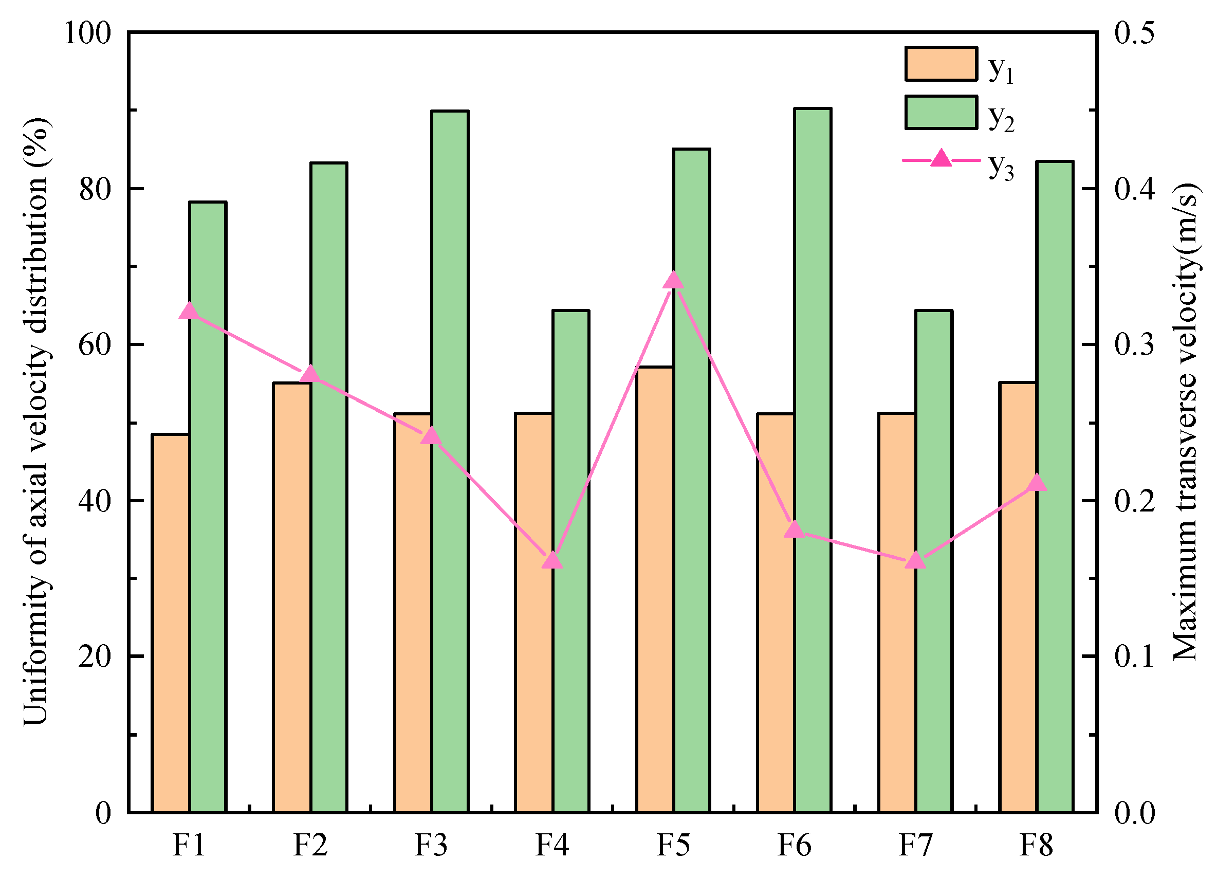
(9)

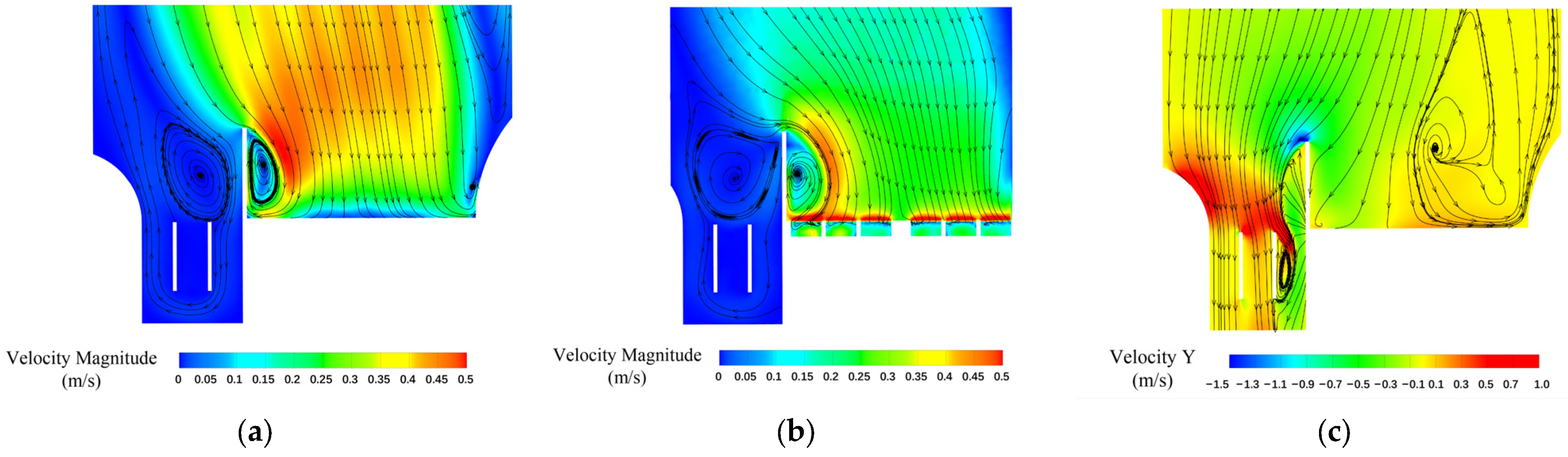
For the four schemes obtained in Step (8) and the scheme optimized by the orthogonal test, numerical simulation was carried out. The uniformity of axial velocity distribution of inlet channel 6#, the flow pattern of sluice 7# and the transverse velocity in front of sluice 9# under six schemes were compared and analyzed so that the scheme of hole parameters could be optimized.

4. Results and Analysis

Based on the changing water levels under different operating conditions, the planar arrangement of the combined sluice-pumping station was shown in Figure 3, the computation range was shown in Figure 7 and the orthogonal testing scheme was shown in Table 1, with 25 distinct calculation models for each of the pumping and self-draining conditions established using the UG software. Figure 11 presents the calculation model for the pumping condition with the hole parameters M × D × H of 1.0 m × 6.25 m × 3.7 m. The Fluent software could be utilized to calculate the hydraulic characteristics of the forebay in the corresponding working conditions for the above 50 combined sluice-pumping station models.

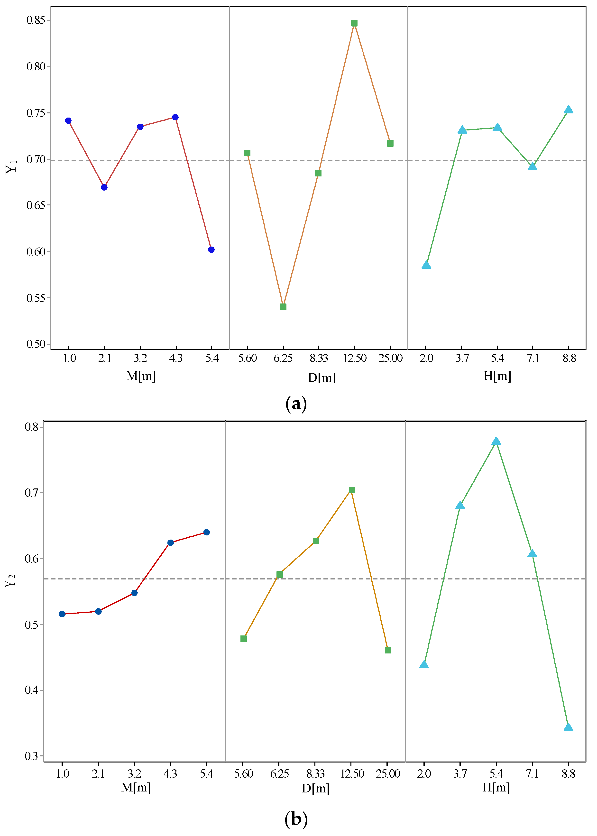
4.1. Analysis of Orthogonal Test Results

Based on the orthogonal experimental design and numerical simulations, the numerical simulation results are presented in

Table 2. Orthogonal table and test results.

Schemes	Parameters Designed			y1	y2	y3
	M (m)	D (m)	H (m)
P1	1.00	5.60	2.00	0.501	0.790	0.284
P2	1.00	6.25	3.70	0.504	0.778	0.325
P3	1.00	8.33	5.40	0.502	0.818	0.317
P4	1.00	12.50	7.10	0.511	0.779	0.352
P5	1.00	25.00	8.80	0.476	0.711	0.337
P6	2.10	5.60	3.70	0.485	0.772	0.251
P7	2.10	6.25	5.40	0.474	0.840	0.254
P8	2.10	8.33	7.10	0.484	0.818	0.237
P9	2.10	12.50	8.80	0.504	0.801	0.252
P10	2.10	25.00	2.00	0.503	0.650	0.369
P11	3.20	5.60	5.40	0.496	0.820	0.210
P12	3.20	6.25	7.10	0.488	0.778	0.225
P13	3.20	8.33	8.80	0.512	0.752	0.218
P14	3.20	12.50	2.00	0.502	0.769	0.262
P15	3.20	25.00	3.70	0.492	0.798	0.296
P16	4.30	5.60	7.10	0.478	0.803	0.192
P17	4.30	6.25	8.80	0.498	0.749	0.174
P18	4.30	8.33	2.00	0.484	0.759	0.260
P19	4.30	12.50	3.70	0.530	0.869	0.252
P20	4.30	25.00	5.40	0.507	0.835	0.320
P21	5.40	5.60	8.80	0.512	0.643	0.163
P22	5.40	6.25	2.00	0.408	0.809	0.238
P23	5.40	8.33	3.70	0.477	0.870	0.225
P24	5.40	12.50	5.40	0.511	0.899	0.235
P25	5.40	25.00	7.10	0.501	0.813	0.287

. Using the mean and extreme deviation, along with main effect plots [20], we evaluated the sensitivity of the indexes to the different test factors.

The results of the experiment were analyzed for polar differences, and the results are shown in

Table 3. Range analysis of test results (pumping condition).

Evaluation Index	Parameter	Factors
		M (m)	D (m)	H (m)
Y1	K1	3.711	3.531	2.927
	K2	3.348	2.704	3.657
	K3	3.678	3.423	3.669
	K4	3.73	4.234	3.457
	K5	3.01	3.585	3.767
	k1	0.742	0.706	0.585
	k2	0.67	0.541	0.731
	k3	0.736	0.685	0.734
	k4	0.746	0.847	0.691
	k5	0.602	0.717	0.753
	R	0.144	0.306	0.168

and

Table 4. Range analysis of test results (self-draining condition).

Evaluation Index	Parameter	Factors
		M (m)	D (m)	H (m)
Y2	K1	2.578	2.389	2.194
	K2	2.6	2.883	3.405
	K3	2.74	3.137	3.892
	K4	3.125	3.525	3.033
	K5	3.2	2.309	1.719
	k1	0.516	0.478	0.439
	k2	0.52	0.577	0.681
	k3	0.548	0.627	0.778
	k4	0.625	0.705	0.607
	k5	0.64	0.462	0.344
	R	0.124	0.243	0.435
Y3	K1	1.104	3.612	2.090
	K2	2.333	3.042	2.396
	K3	3.073	2.847	2.459
	K4	3.135	2.380	2.673
	K5	3.372	1.136	3.399
	k1	0.221	0.722	0.418
	k2	0.467	0.608	0.479
	k3	0.615	0.569	0.492
	k4	0.627	0.476	0.535
	k5	0.674	0.227	0.680
	R	0.453	0.495	0.262

, where K_i indicates the sum of evaluation indicators at level i for each column of factors, k_i is the mean value of K_i and the extreme difference value R = max(k_i) − min(k_i). The extreme difference analysis revealed that the degree of influence of each factor on Y₁ in this test (from large to small) were the hole center distance D, the hole depth H and the hole width M. The degree of influence of each factor on Y₂ (from large to small) were the hole depth H, the hole center distance D and the hole width M. The degree of influence of each factor on Y₃ (from large to small) were the hole center distance D, the hole width M and the hole depth H.

The main effect analysis method can be used to study the influence of hole parameters (M, D and H) on the three evaluation indicators (Y₁, Y₂ and Y₃) and obtain the corresponding hole parameters when the evaluation indicators are optimal. The relationship between Y₁, Y₂ and Y₃ and hole parameters is shown in Figure 12, where the horizontal coordinate is the five horizontal values of each factor and the vertical coordinate is the average value of each indicator after normalization under the corresponding factor level. The dotted line in the figure is the average value of each index.

It can be seen from Figure 12 that the effect of hole parameters on Y₁, Y₂ and Y₃ is different. For the evaluation indexes Y₁ and Y₃, the most influencing factor is D, while factor M and H show relatively little impact. With an increase in D, the evaluation indicator Y₁ fluctuates, while Y₃ shows a decreasing trend. For evaluation indicator Y₂, the most influencing factor is H. Specifically, with an increase in H, Y₂ first increases from 0.44 to 0.78, followed by a decline of 0.44. According to Figure 12, to make the evaluation index Y₁ maximum possible, M should be taken as 4.3 m, D should be taken as 12.5 m and H should be taken as 8.8 m. To make the evaluation indicator Y₂ maximum possible, M should be taken as 5.4 m, D should be taken as 12.5 m and H should be taken as 5.4 m. To make the evaluation index Y₃ maximum possible, M should be taken as 5.4 m, D should be taken as 5.6 m and H should be taken as 8.8 m.

To summarize, the effect of hole parameters on Y₁, Y₂ and Y₃ is different, and the corresponding hole parameters are also diverse when Y₁, Y₂ and Y₃ reach the maximum value. In fact, it is impossible for Y₁, Y₂ and Y₃ to get the maximum value at the same time, so it is necessary to adopt the multi-objective optimization method for further optimization research.

4.2. Calculation of Weight Coefficients and Establishment of Comprehensive Evaluation Indicators

According to the variation coefficient method used to calculate the weight coefficients, the results are presented in

Table 5. Calculation table of weighting coefficients.

Schemes	Parameters Designed			Y1	Y2	Y3	Y
	M (m)	D (m)	H (m)
P1	1.00	5.60	2.00	0.763	0.573	0.410	0.546
P2	1.00	6.25	3.70	0.782	0.528	0.210	0.449
P3	1.00	8.33	5.40	0.769	0.684	0.251	0.518
P4	1.00	12.50	7.10	0.844	0.531	0.080	0.408
P5	1.00	25.00	8.80	0.553	0.263	0.154	0.281
P6	2.10	5.60	3.70	0.628	0.502	0.571	0.560
P7	2.10	6.25	5.40	0.536	0.768	0.556	0.625
P8	2.10	8.33	7.10	0.622	0.685	0.640	0.652
P9	2.10	12.50	8.80	0.783	0.618	0.566	0.633
P10	2.10	25.00	2.00	0.779	0.027	0.000	0.184
P11	3.20	5.60	5.40	0.719	0.690	0.771	0.731
P12	3.20	6.25	7.10	0.655	0.527	0.697	0.628
P13	3.20	8.33	8.80	0.852	0.426	0.733	0.653
P14	3.20	12.50	2.00	0.768	0.493	0.520	0.566
P15	3.20	25.00	3.70	0.684	0.604	0.353	0.514
P16	4.30	5.60	7.10	0.574	0.624	0.861	0.714
P17	4.30	6.25	8.80	0.731	0.413	0.947	0.713
P18	4.30	8.33	2.00	0.618	0.455	0.528	0.522
P19	4.30	12.50	3.70	1.000	0.884	0.566	0.774
P20	4.30	25.00	5.40	0.807	0.750	0.234	0.542
P21	5.40	5.60	8.80	0.847	0.000	1.000	0.618
P22	5.40	6.25	2.00	0.000	0.647	0.633	0.496
P23	5.40	8.33	3.70	0.562	0.887	0.696	0.732
P24	5.40	12.50	5.40	0.839	1.000	0.648	0.813
P25	5.40	25.00	7.10	0.762	0.666	0.396	0.572
Standard Deviation				0.181	0.229	0.257
Coefficient of Variation				0.259	0.401	0.494
Weight Coefficient				0.224	0.348	0.428

. The optimization of the hole parameters on the diversion wall is expected to improve the flow pattern of inlet channel 6# under pumping conditions and to result in smoother flow in sluice chamber 7# and lower transverse velocity in the sluice area ahead of the navigable sluice chamber 9# under self-draining conditions. Notably, the larger the Y value, the better the operational state of the combined sluice-pumping station project.

According to the calculation results in Table 5, the equation of comprehensive evaluation indicator is shown in Equation (15)

$$Y=0.224Y_1+0.348Y_2+0.482Y_3$$

(15)

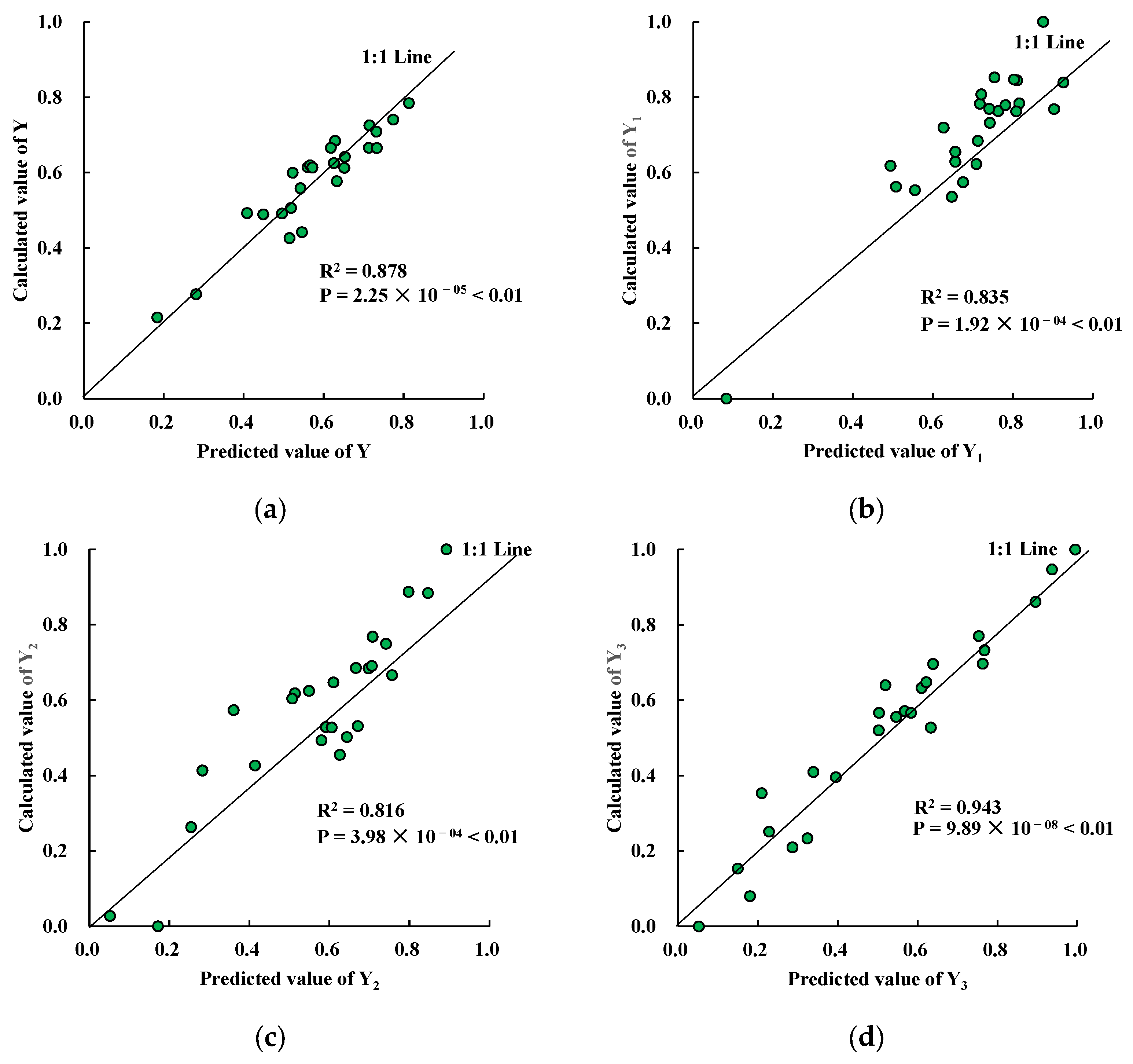
4.3. Regression Modeling Based on Response Surface Methodology

Regression equations between each evaluation indicator and the perforation parameters were established using the least square method, based on the results of the orthogonal experiment.

The regression equation of evaluation indicator Y is shown as follows:

$$\begin{array}{cc}Y& =0.4419+0.5788A+0.3601B+0.2639C-0.1068AB+0.4465AC+\hfill \\ & 0.4248BC-0.5363A^2-0.702B^2-0.5294C^2\hfill \end{array}$$

(16)

The regression equation of Y₁ is shown as follows:

$$\begin{array}{cc}{Y}_1& =0.763-0.2654A+1.94B-0.3205C-0.4064AB+1.573AC+\hfill \\ & 0.397BC-0.463A^2-1.775B^2-0.4851C^2\hfill \end{array}$$

(17)

The regression equation of Y₂ is shown as follows:

$$\begin{array}{cc}{Y}_2\hfill & =0.3607+0.3947A+0.1996B+1.177C+0.4888AB-0.4228AC+\hfill \\ & 0.4156BC-0.1669A^2-0.7537B^2-1.171C^2\hfill \end{array}$$

(18)

The regression equation of Y₃ is shown as follows:

$$\begin{array}{cc}{Y}_3\hfill & =0.3397+1.171A-0.3374B-0.1714C-0.4335AB+0.5624AC+\hfill \\ & 0.4469BC-0.8746A^2-0.09812B^2-0.03159C^2\hfill \end{array}$$

(19)

In Equations (16)–(19), A, B and C were the normalized variables of the perforation parameters of the diversion wall, which were calculated by Equations (20)–(22).

$$A=\frac{M-1}{4.4}$$

(20)

$$B=\frac{D-5.6}{19.4}$$

(21)

$$C=\frac{H-2}{6.8}$$

(22)

As shown in Figure 13, the predicted values and the calculated values from the numerical simulation are plotted against each other. The points are clustered around the 1:1 line, which suggests a high degree of model fit. The composite objective function Y had a response surface model with a coefficient of determination of 0.878. This implies that the model can explain 87.8% of the variation in the data. The model was also highly significant, as its p-value of 2.25 × 10⁻⁵ is much lower than 0.01. The coefficients of determination for the individual objective functions Y₁, Y₂ and Y₃ were 0.835, 0.816 and 0.943 respectively. These values are all above 0.8, which indicates that the models have a good fit as well.

4.4. Analysis of the Impact of Hole Parameters on the Evaluation Index Based on Response Surface Model

Figure 14, Figure 15, Figure 16 and Figure 17 (respectively) depict the response surface plots of two parameters and the target value when a certain parameter is fixed at the intermediate level. In Figure 14, Figure 15, Figure 16 and Figure 17, A, B and C are the normalized values of H, M and D, respectively. If there is no interaction between H, M and D, the contours on the response surface plot should appear as concentric circles. Conversely, if the contours on the response surface plot are strongly distorted, it indicates a strong interaction between the two factors.

As can be seen from Figure 14, Figure 15, Figure 16 and Figure 17, the three hole parameters have a strong interaction effect on each evaluation indicator. For the overall evaluation indicator Y, as H increases, the optimal values of M and D also gradually increase. Within the range of values that contains the maximum value of the overall evaluation indicator Y, when M is at a high level (around 0.8), D is at a medium level (around 0.5) and H is at a relatively high level (around 0.65), Y can reach its maximum value. The fastest ascent method can be used to find the maximum values of each response surface model in the calculation region, and the results are listed in

Table 6. Optimization results of different hole parameters.

Scheme	Method		Optimization Objectives	M [m]	D [m]	H [m]	y1 [%]	y2 [%]	y3 [m/s]
F1	/	/		/	/	/	48.5	78.3	0.32
F2	Main Effect Analysis		Y1	4.3	12.5	8.8	55.0	83.2	0.28
F3			Y2	5.4	12.5	5.4	51.1	89.9	0.24
F4			Y3	5.4	5.6	8.8	51.2	64.3	0.16
F5	Response Surface Methodology		Y1	5.4	15.9	8.8	57.1	85.1	0.34
F6			Y2	5.4	16.5	4.9	51.1	90.3	0.18
F7			Y3	5.4	5.6	8.8	51.2	64.3	0.16
F8			Y	4.6	14.1	7.2	55.1	83.5	0.21

.

4.5. Optimization Results and Validation of Hole Parameters

Numerical simulation experiments were conducted on the original scheme, three optimization schemes obtained by main effect analysis and four optimization schemes obtained by response surface analysis. The results of the numerical simulation are shown in Table 6 and Figure 18, where F1 represents the original scheme with the diversion wall non-perforated. F2–F4 represent the aperture schemes obtained by main effect analysis with Y₁, Y₂ and Y₃ as optimization objectives, respectively. F5–F8 represent the aperture schemes obtained by response surface analysis with Y₁, Y₂, Y₃ and Y as optimization objectives, respectively. Figure 19, Figure 20, Figure 21, Figure 22, Figure 23, Figure 24, Figure 25 and Figure 26 display the flow pattern under pumping and self-draining conditions for each of the abovementioned schemes.

The results of numerical simulation experiments indicate that appropriate holes on the diversion wall can improve the uniformity of axial flow velocity distribution and reduce the transverse flow velocity under self-draining and pumping conditions, so that the flow state of the forebay in the combined sluice-pumping station project can be improved. The hole scheme in F8 obtained by adopting the response surface analysis method and taking the comprehensive evaluation indicator as the optimization objective was found to result in an improvement in the uniformity of axial flow velocity distribution in inlet channel 6# by 6.6% and in sluice chamber 7# by 5.2% compared to the original scheme F1. Additionally, the maximum transverse flow velocity decreased from 0.32 m/s to 0.21 m/s, which is a reduction of 34.4%. After a series of calculations and comparisons, the optimized solution met the navigation requirements.

4.6. Discussion

As shown by the results of numerical simulation calculations for the optimization scheme, creating reasonable holes on the diversion wall can improve the flow state of the forebay in the combined sluice-pumping station project. As seen in Figure 19, under the pumping condition, the original design without holes on the diversion wall leads to a large area of backflow forming in front of inlet channel 6#, forcing the flow to deviate from the channel and affecting the flow state of the pumping station. Under the self-draining condition, the backflow area occurs near the junction of the sluice and the diversion wall, affecting the flow state in the sluice chamber. Compared to the original scheme, the optimization target y₁ increased by 6.5% under the optimization scheme F2, and there was also some improvement in the non-optimization targets y₂ and y₃. As seen in Figure 20, Figure 21, Figure 22, Figure 23, Figure 24, Figure 25 and Figure 26, it can be inferred that the holes in the diversion wall have a smoothing effect on the flow, dispelling the backflow area and improving the flow state in the forebay. This smoothing effect not only improves the flow state under pumping conditions, but it also has a positive effect on the flow state under self-draining conditions.

The main effect analysis method can only perform optimization at the level of orthogonal experimental design. Therefore, for the same optimization objective, the response surface analysis method has a more significant optimization effect and more precise optimization parameters compared to the main effect analysis method. The F3 and F6 optimization schemes were obtained using the main effect analysis method and single-objective response surface analysis method, respectively, with y₂ as the optimization objective. The y₂ value of the F6 scheme was better than that of the F3 scheme. However, the single-objective response surface analysis method may result in worse non-objective values while obtaining a better objective value. For example, compared to F2, the target value y₁ increased by 2.1% in the F5 scheme, but the maximum transverse flow velocity increased from 0.24 m/s to 0.34 m/s, which does not meet the navigation requirements [29].

The utilization of the comprehensive evaluation indicator Y (multi-objective optimization) leads to a more balanced and reasonable hole scheme compared to single-objective optimization. For instance, adopting the single-objective response surface optimization for F5 results in the highest y₁ value among all the schemes, but it results in an unacceptably high y₃ of 0.34 m/s for safe navigation of ships. When the F6 optimization with a single-objective response surface makes y₂ optimal, y₁ is only 51.1%, and under the F7 scheme, the numerical simulation result of the optimization index y₃ is 0.16 m/s, while y₂ is only 64.3%.

In conclusion, the response surface method proves to be an efficient optimization technique in engineering structure design. Adopting comprehensive evaluation indexes is crucial in accounting for multiple objectives in the optimization process. The evaluation indexes and response surface method adopted in this study offer useful insights for analyzing the hydraulic characteristics and optimizing the design of the inlet and outlet structures in the combined sluice-pumping station project. This methodology is deserving of further consideration and promotion in future studies.

5. Conclusions

In this study, the optimal hole parameters of the diversion wall were sought. The design of experiments was carried out by adopting the orthogonal test method, and numerical simulations were performed using numerical simulation software for the combined sluice-pumping station. A set of comprehensive evaluation indexes were proposed. Based on the response surface analysis of the evaluation indexes on the experimental data, the relationship between the comprehensive evaluation indexes and the hole parameters of the diversion wall was established, resulting in the development of a method and theory for optimizing the hole parameters of the diversion wall in the combined sluice-pumping station. The following main conclusions were obtained from this research:

(1)

Utilization of the coefficient of variation method enables a comprehensive evaluation of the flow state assessment indexes of the combined sluice-pumping station under different operating conditions. This leads to a more reasonable evaluation of the operation status of the combined sluice-pumping station. By combining the orthogonal experimental design and response surface analysis, a second-order polynomial function relating the hole parameters of the diversion wall to the response values is established. The optimization parameters for the hole obtained through the steepest ascent method to obtain the maximum value are more efficient and accurate.

(2)

The numerical simulation results demonstrate the feasibility of the method of the comprehensive evaluation indicator combined with the response surface method. The optimization of the hole parameters obtained by this method is more balanced and reasonable compared to other single-objective optimization methods. The final optimization parameters of the hole are as follows: hole width 4.6 m, hole center distance 14.1 m and hole depth 7.2 m. Compared to the original scheme, the uniformity of axial velocity distribution in inlet channel #6 improved by 6.6%, the uniformity of axial velocity distribution in chamber #7 improved by 5.2% and the maximum transverse velocity decreased by 34.4%. Hence, the combined sluice-pumping station project met the navigation requirements after optimization.

(3)

The response surface methodology and the methodology that employs the variance coefficient to calculate weights were shown to be effective optimization approaches. In the context of engineering structure optimization, it is crucial to synthesize all relevant evaluation indexes. The methodologies proposed in this study can provide guidance for analyzing hydraulic characteristics, selecting corrective measures and optimizing the inlet and outlet structures in combined sluice-pumping stations. Although the case study is limited to a specific geometry, the evaluation index selection method and optimization methodology proposed in this study are valuable and can be adapted to other engineering structures based on their specific characteristics. Given the benefits of these evaluation indicator selection and optimization design methodologies, they deserve further promotion and consideration.

(4)

In the forthcoming stage, physical model tests will be performed to verify the optimized outcomes. Furthermore, the research will delve into novel forms of the diversion wall structure and optimization techniques, offering guidance and technical assistance for the hydraulic analysis of the inlet and outlet structures, optimization design and selection of rectifying measures in the combined sluice-pumping station project.

(5)

Our research demonstrated that the perforated diversion wall is an effective solution for improving flow conditions in the forebay under certain operating conditions. However, it is important to note that our study only considered a limited range of operating conditions. Further optimization is needed to ensure reliable operation of the wall under a wider range of water levels and pump unit activations. Therefore, future studies should focus on optimizing the perforated diversion wall for more common operating conditions to ensure good flow conditions in the forebay under all operating conditions.

References

- Yan, Z.; Zhou, C.; Yan, W.; Zhang, P. Study on the Layout of Combined Sluice-Pump Station Projects and Modification of Flow Pattern. Hehai Daxue Xuebao Ziran Kexueban 2000, 28, 50–53. [Google Scholar]
- Spence, R.; Amaral-Teixeira, J. Investigation into pressure pulsations in a centrifugal pump using numerical methods supported by industrial tests. Comput. Fluids 2008, 37, 690–704. [Google Scholar] [CrossRef]
- Xu, B.; Liu, J.; Lu, W.; Xu, L.; Xu, R. Design and Optimization of γ-Shaped Settlement Training Wall Based on Numerical Simulation and CCD-Response Surface Method. Processes 2022, 10, 1201. [Google Scholar] [CrossRef]
- Song, W.W.; Pang, Y.; Shi, X.H.; Xu, Q. Study on the Rectification of Forebay in Pumping Station. Math. Probl. Eng. 2018, 2018, 2876980. [Google Scholar] [CrossRef]
- Xi, W.; Lu, W.; Wang, C.; Xu, B. Optimization of the Hollow Rectification Sill in the Forebay of the Pump Station Based on the PSO-GP Collaborative Algorithm. Shock. Vib. 2021, 2021, 6618280. [Google Scholar] [CrossRef]
- Liu, C. Pump and Pumping Station; China Water & Power Press: Beijing, China, 2009; pp. 77–86. [Google Scholar]
- Montes, J.S. Irrotational flow and real fluid effects under planar sluice gates-Closure. J. Hydraul. Eng.-ASCE 1999, 125, 212–213. [Google Scholar]
- Speerli, J.; Hager, W.H. Irrotational flow and real fluid effects under planar sluice gates-Discussion. J. Hydraul. Eng.-ASCE 1999, 125, 208–210. [Google Scholar]
- Chen, Y.J.; Yang, J.; Yu, J.Z.; Fu, Z.F.; Chen, Q.S. Flow Expansion and Deflection Downstream of a Symmetric Multi-gate Sluice Structure. KSCE J. Civ. Eng. 2020, 24, 471–482. [Google Scholar] [CrossRef]
- Mohamed, I.M.; Abdelhaleem, F.S. Flow Downstream Sluice Gate with Orifice. KSCE J. Civ. Eng. 2020, 24, 3692–3702. [Google Scholar] [CrossRef]
- Luo, C.; Qian, J.; Liu, C.; Chen, F.; Xu, J.; Zhou, J. Numerical simulation and test verification on diversion pier rectifying flow in forebay of pumping station for asymmetric combined sluice-pump station project. Trans. Chin. Soc. Agric. Eng. 2015, 31, 100–108. [Google Scholar]
- Luo, C.; Liu, C. Numerical simulation and improvement of side-intake characteristics of multi-unit pumping station. J. Hydroelectr. Eng. 2015, 34, 207–214. [Google Scholar]
- Luo, C.; He, Y.; Shang, Y.; Cong, X.; Ding, C.; Cheng, L.; Lei, S. Flow Characteristics and Anti-Vortex in a Pump Station with Laterally Asymmetric Inflow. Processes 2022, 10, 2398. [Google Scholar] [CrossRef]
- Yang, F.; Zhang, Y.; Liu, C.; Wang, T.; Jiang, D.; Jin, Y. Numerical and Experimental Investigations of Flow Pattern and Anti-Vortex Measures of Forebay in a Multi-Unit Pumping Station. Water 2021, 13, 935. [Google Scholar] [CrossRef]
- Wang, X.; Feng, J.; Fu, L. Study on the rectification measures of the forebay of the pumping station of the sluice station in the tidal river section. China Rural. Water Hydropower 2013, 366, 140–143. [Google Scholar]
- Fu, Z.; Gu, M.; Yan, Z. Shape and suitable length for guide wall of combined sluice-pump station project. Water Resour. Hydropower Eng. 2011, 42, 128–131. [Google Scholar]
- Xu, B.; Zhang, C.; Xia, H.; Gao, C.; Liu, P. A Test Research on the Flow Condition Model in Forebay of Pumping Station for Asymmertric Combined Sluice-pump Station Project. Water Resour. Power 2018, 36, 132, 160–162. [Google Scholar]
- Xu, B.; Yao, T.; Xia, H.; Gao, C. Experimental research on opening diversion piers at Xifeihe combined sluice-pump station. Hydro-Sci. Eng. 2018, 172, 55–61. [Google Scholar]
- Xu, B.; Zhang, C.; Li, Z.; Gao, C.; Bi, C. Using CFD Model to Analyze the Influence of Geometric Parameters of Diversion Piers on Water Flow in Sluice Station. J. Irrig. Drain. 2019, 38, 115–122. [Google Scholar]
- Xu, B.; Liu, J.F.; Lu, W.G. Optimization Design of Y-Shaped Settling Diversion Wall Based on Orthogonal Test. Machines 2022, 10, 91. [Google Scholar] [CrossRef]
- Cheng, L.; Qi, W.; Luo, C.; Shang, Y.; Yuan, H. Effect of geometric parameters of Y-shaped diversion piers on flow pattern in forebay of pumping station. Adv. Sci. Technol. Water Resour. 2014, 34, 68–72. [Google Scholar]
- Zhou, J.R.; Zhao, M.M.; Wang, C.; Gao, Z.J. Optimal Design of Diversion Piers of Lateral Intake Pumping Station Based on Orthogonal Test. Shock. Vib. 2021, 2021, 6616456. [Google Scholar] [CrossRef]
- Xu, W.; Cheng, L.; Du, K.; Yu, L.; Ge, Y.; Zhang, J. Numerical and Experimental Research on Rectification Measures for a Contraction Diversion Pier in a Pumping Station. J. Mar. Sci. Eng. 2022, 10, 1437. [Google Scholar] [CrossRef]
- Chen, G. Study on the Influence of Diversion Pier on the Hydraulic Characteristics of Xifeihe Combined-sluice Pump Project. Master’s Thesis, Yangzhou University, Yangzhou, China, 2018. [Google Scholar]
- Wang, F.; Tang, X.; Chen, X.; Xiao, R.; Yao, Z.; Yang, W. A review on flow analysis method for pumping stations. J. Hydraul. Eng. 2018, 49, 47–61, 71. [Google Scholar]
- Xu, L.; Lu, W.G.; Lu, L.G.; Dong, L.; Wang, Z.F. Flow patterns and boundary conditions for inlet and outlet conduits of large pump system with low head. Appl. Math. Mech.-Engl. 2014, 35, 675–688. [Google Scholar] [CrossRef]
- Zhou, J.R.; Zhao, M.M.; Wang, C.; Gao, Z.J. Influence of Different Lateral Bending Angles on the Flow Pattern of Pumping Station Lateral Inflow. Shock. Vib. 2021, 2021, 6653001. [Google Scholar] [CrossRef]
- Mulligan, K.B.; Towler, B.; Haro, A.; Ahlfeld, D.P. A computational fluid dynamics modeling study of guide walls for downstream fish passage. Ecol. Eng. 2017, 99, 324–332. [Google Scholar] [CrossRef]
- JTJ 305-2001; Code for Master Design of Shiplocks. Ministry of Transport of the People’s Republic of China: Beijing, China, 2001.
- Sangsefidi, Y.; MacVicar, B.; Ghodsian, M.; Mehraein, M.; Torabi, M.; Savage, B.M. Evaluation of flow characteristics in labyrinth weirs using response surface methodology. Flow Meas. Instrum. 2019, 69, 101617. [Google Scholar] [CrossRef]
- Shan, Z.; Long, J.; Yu, P.; Shao, L.; Liao, Y. Lightweight optimization of passenger car seat frame based on grey relational analysis and optimized coefficient of variation. Struct. Multidiscip. Optim. 2020, 62, 3429–3455. [Google Scholar] [CrossRef]
- Yan, J.; Li, L. Multi-objective optimization of milling parameters – the trade-offs between energy, production rate and cutting quality. J. Clean. Prod. 2013, 52, 462–471. [Google Scholar] [CrossRef]