Theory and Application of Geostatistical Inversion: A Facies-Constrained MCMC Algorithm

Abstract

To improve the prediction of thin reservoirs with special geophysical responses, a geostatistical inversion technique is proposed based on an in-depth analysis of the theory of geostatistical inversion. This technique is based on the Markov chain Monte Carlo algorithm, to which we added the contents of facies-constrained. The feasibility of the technique and the reliability of the prediction results are demonstrated by a prediction of the sand bodies in the braided river channel bars in the Xiazijie Oilfield in the Junggar Basin. Based on the MCMC algorithm, the results show that leveraging the lateral changes in the seismic waveforms as geologically relevant information to drive the construction of the variogram and the optimization of the statistical sampling can largely overcome the obstacle that prevents traditional geostatistical inversions from accurately delineating the sedimentary characteristics; thereby, the proposed algorithm truly achieves facies-constrained geostatistical inversion. The case study of the Xiazijie Oilfield showed the feasibility and reliability of this technology. The prediction accuracy of the FCMCMC algorithm-based geostatistical inversion is as high as 6 m for thin interbedded reservoirs, and the coincidence rate between the prediction results and the well log data is more than 85%, which confirms the reliability of the technique. The demonstrated performance of the proposed technique provides a preliminary reference for the prediction of the thin interbedded reservoirs formed in terrestrial sedimentary basins and characterized by small thicknesses and rapid lateral changes with special geophysical responses.

1. Introduction

As oil and gas exploration continues to advance, more attention is being paid to the prediction and evaluation of reservoirs with special petrophysical characteristics. This is an important direction for future oil and gas exploration. The target reservoirs include igneous rocks, metamorphic rocks, weathered crusts, mudstones, shales, conglomerates, and thin sandstone–mudstone interbeds [1,2,3,4,5]. These reservoirs are formed under complex conditions, which lead to diverse reservoir spaces and strong spatial non-homogeneity, thereby resulting in extremely complex petrophysical properties [6,7,8]. As a result, it is impossible to rely on the acoustic transit time, density, acoustic impedance, and elastic parameters to effectively distinguish between reservoir and non-reservoir units. Accordingly, it is difficult to predict these reservoirs by means of conventional pre-stack and post-stack inversions, and it is particularly difficult to predict the spread of thin reservoirs with special petrophysical properties using conventional inversion techniques [9,10,11]. Seismic wave attenuation, which is known for its high sensitivity to the physical properties of rocks, has shown success in the lateral delineation of thin reservoirs [12]. However, as explained by Matsushima et al. in 2017, the estimation of seismic attenuation is challenging, especially in carbonate reservoirs [13,14], despite several studies carried out to improve the methodology [15].

At present, efforts are being made to overcome the above obstacles through two main approaches. The first is nonlinear inversion, which mainly involves artificial neural networks, principal component analysis, and support vector machines. The theory of nonlinear inversion is that under the constraints of geological models, the nonlinear relationship between the borehole lithology data and the seismic data is established using mathematical algorithms, followed by the processing of the lithologic parameters based on known statistical relationships, in order to derive the reservoir’s electrical parameters (e.g., the natural gamma radiation, spontaneous potential (SP), and electrical resistivity) and the reservoir’s physical parameters (e.g., the porosity, permeability, and saturation) [16,17,18,19]. This technique overcomes the inherent resolution limitations of the seismic data and thereby provides high-precision inversion results. However, the inversion algorithms involved lack clear physical meanings and the relationships between the electrical parameters and the seismic information are not clear, which suggests that this technique is theoretically flawed to some extent and thereby subject to limitations in terms of its development and application [20,21,22,23]. The second approach is geostatistical inversion, which mainly involves sequential Gaussian simulation algorithms and Markov chain Monte Carlo (MCMC) algorithms. Sequential Gaussian simulation algorithms are the main type of algorithm used in the early version of geostatistical inversion, and their implementation involves the following steps. First, the conditional data are converted into standard Gaussian values. This is followed by the conversion of the values to a variogram; the obtaining of the Kriging estimate and variance at each node according to the simulated data and conditional data; the determination of the conditional Gaussian distribution; the random sampling of the distribution to obtain a series of reservoir parameter models; and, finally, the conversion of the Gaussian simulation results into the original data to obtain the continuous distributions of the reservoir’s electrical and physical properties. However, the second technique has some limitations, which limit its development and application [24,25,26]. Firstly, the algorithms provide final, yet approximate, results immediately when all of the grid cells are filled; so, the results are not strictly correct in a statistical sense. Secondly, the repeated single-trace simulation involved in the algorithms leads to a low computational efficiency.

The MCMC algorithms have emerged in recent years and have been widely used for numerical computation. Because the MCMC algorithms are suitable for simulating distributions that are multivariate and non-standard or even have mutually dependent variables, they are applicable to reservoir prediction [27,28,29,30]. Their implementation involves the following steps. First, a probability density function is determined through statistical analysis. This is followed by the use of Bayesian inference to obtain the above-mentioned information; the defining of the posterior probability distribution function of the reservoir; the simulation of the Markov chain sampling according to the probability distribution function to obtain a sequence of data points with statistical significance; and the estimation of the expected values of the distributions of the reservoir’s parameters (e.g., the lithological and physical parameters of the reservoir) via Monte Carlo integration based on the above sequences. Compared with the sequential Gaussian simulation algorithms, the MCMC algorithms have a higher computational efficiency and involve a more rigorous calculation process; thereby, they can effectively avoid local optimization, leading to their wide application in recent years in lithology inversion and thin reservoir prediction in the field of petroleum exploration and extraction [31,32]. However, the current MCMC algorithm-based geostatistical inversion technique relies on the distance range of known well locations to select the optimal samples for simulation, which achieves only a rough delineation of the spatial heterogeneity and fails to reflect the changes in the characteristics of the facies. That is, the sampling optimization in the current MCMC algorithm-based geostatistical inversion technique is only distance-dependent and lacks a clear geological relevance, which is obviously inconsistent with the sedimentary characteristics of the research objects. In order to overcome this problem, in this study a geostatistical inversion technique that integrates a facies-constrained MCMC (FCMCMC) algorithm was developed. Based on the facts that seismic data are laterally continuous and that changes in the seismic waveforms reflect changes in the sedimentary environment, the FCMCMC leverages the lateral changes in the seismic waveforms to drive the construction of the variogram and to constrain the selection of the sample points in order to ensure that the inversion results have a sedimentary relevance.

The theory of the FCMCMC algorithm-based geostatistical inversion is presented, and then, the proposed technique is used to predict the reservoirs in the Xiazijie Oilfield in the Junggar Basin. This technique was used to successfully predict the distribution characteristics of the sand bodies in the braided river channel bars of the Jurassic Badaowan Formation in the Xiazijie Oilfield. The prediction results are in good agreement with the log data from the validation wells and are consistent with the sedimentary patterns of the study area. Finally, the reliability of the prediction results and the scientific soundness of this technique are confirmed through borehole logging. The theory and demonstrated performance of the FCMCMC algorithm-based geostatistical technique developed in this study provide a reference for the study of facies-constrained inversion and the prediction of thin reservoirs with special petrophysical properties in other areas.

2. Theory and Methodology of the Inversion Technique

In this study, a geostatistical inversion technique based on an FCMCMC algorithm was developed. The biggest improvement lies in the proposal to constrain the selection of samples in the inversion process by using the sedimentary significance represented by seismic waveforms. The purpose is to make the inversion results have geological concepts. The implementation of this technique involves the following steps.

• It uses 3D seismic data cubes, borehole core data, well logs, and waveform clustering analysis or coherence analysis to determine the distribution characteristics of the seismic facies, which can indirectly reflect the horizontal distribution of the sedimentary facies.
• Under the constraints provided by the seismic facies distribution, statistical analysis is performed based on variograms to determine the prior probability density function, which is then used in the Bayesian inference framework to define the posterior probability distribution function of the reservoir.
• Based on the probability distribution function, an MCMC algorithm is used to perform Markov chain sampling to obtain a sequence of target sample points, followed by the use of the Monte Carlo integration to calculate the expected value of these samples in order to obtain the electrical and physical parameters, which can reflect the spatial distribution characteristics of the reservoir.

2.1. Establishing the Objective Function

According to the definition of the Bayesian conditional probability, the posterior probability of an event is

$$p\left(m|n\right)=\frac{p\left(n,m\right)}{p\left(n\right)}=\frac{p\left(n|m\right)p\left(m\right)}{{\displaystyle \int p\left(n|m\right)}p\left(m\right)dm}\propto p\left(m\right)p\left(n|m\right)$$

(1)

where m is a model parameter; n is an observation sample; p(m) is the prior distribution of m, which is independent of n and can be obtained from the well log data; p(n) is the probability of the occurrence of n; p(n, m) is the joint distribution of m and n; p(n|m) is the posterior probability of the model after the observation of sample n.

According to exploration seismology, the acoustic impedance calculated from the acoustic logging data is related to the actual acoustic impedance, as follows:

$$Z_{\mathrm{w}}=Z+N$$

(2)

where Z_w is the acoustic impedance calculated from the acoustic logging data, and Z is the actual acoustic impedance.

N is the random noise, which is assumed to have a Gaussian distribution with a mean of 0 and a standard deviation of σ.

Given that ${\Vert Z_W-Z\Vert }^2$ has a Gaussian distribution, as is the case with N, its objective function can be defined as

$$J_1=\frac{{\Vert Z_W-Z\Vert }^2}{2{\sigma }^2}$$

(3)

where σ is the standard deviation of random noise N. In order to reduce the instability and multiplicity of the inversion problem’s solution and to obtain a stable numerical solution, it is necessary to introduce prior information into the objective function in order to constrain it. When performing the maximum posterior estimation, the objective function is

$$J\left(Z\right)=J_1\left(Z\right)+{\lambda }^2{J}_2\left(Z\right)$$

(4)

where J₁(Z) is a function related to the posterior information; J₂(Z) is a prior term, which is a function related to the log data and the geological information; and λ is a smoothing parameter, i.e., a constant that balances the interaction between J₁(Z) and J₂(Z).

According to Equation (2), Equation (3) can be combined as

$$J\left(Z\right)=\frac{{\Vert Z_W-Z\Vert }^2}{2{\sigma }^2}+{\lambda }^2{\phi }^{\mathrm{k}}\left(Z\right)=\frac{{\Vert Z_W-Z\Vert }^2}{2{\sigma }^2}+{\lambda }^2{\displaystyle \sum _C\phi \left(D_c^k\left(Z\right)/\delta \right)}$$

(5)

where φ is a potential function; δ is a scale parameter that adjusts the gradient at the discontinuity; and k is a constant that can be set as 1, 2, or 3. When k = 1, the prior terms are summed over all of the regions that are horizontally and vertically closest to the prediction point; and when k = 2 or 3, the gradients and Hessian matrices between two adjacent points on a plane or a quadratic surface are summed [33,34,35].

2.2. FCMCMC Algorithm-Based Statistical Sampling Optimization

2.2.1. Sample Optimization under the Constraint of Sedimentary Facies

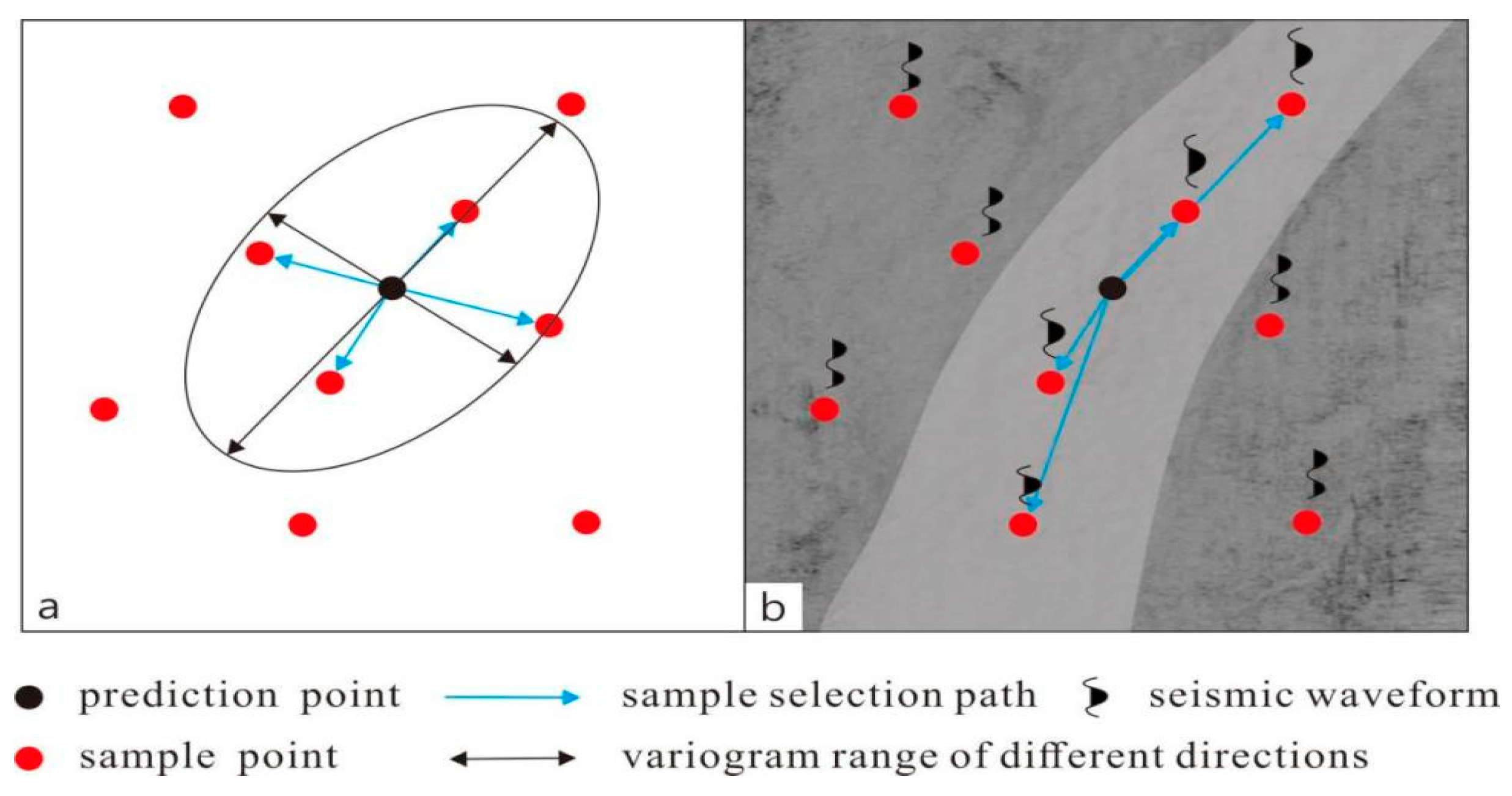
The existing MCMC algorithms rely on the distance range of the samples to perform the statistical sampling optimization. As is shown in Figure 1a, the four sample points that are around the prediction point and within the variogram range are selected as the optimal sample points. This selection scheme only considers the distances from the sample points to the prediction point, regardless of the geological properties at the sample points, and thus, it fails to obtain inversion results that are geologically relevant.

According to seismic stratigraphy and seismic sedimentology, the reflected seismic waveforms can reveal the vertical characteristics of the lithologic association, and such characteristics can be mapped on a horizontal plane (e.g., in a plan view) to illustrate the lateral changes in the sedimentary environment. Therefore, it is possible to use the spatial changes in the seismic waveforms to constrain the variogram construction and the sampling site selection in order to delineate the characteristics of the spatial changes in the target reservoir, which will give the geostatistical inversion results sedimentary relevance and thereby allow for facies-constrained stochastic simulation. Accordingly, in this study the statistical sampling optimization was performed under the constraints provided by the seismic waveform attributes instead of the traditional, variogram-based spatial geostatistical analysis (Figure 1b). The implementation of this new method involves the following steps. First, the seismic waveforms at each sample point and the prediction point are extracted. This is followed by the computation of the waveform correlation coefficient of the prediction point with respect to each sample point; the sorting of the sample points in the order of their waveform correlation coefficients; and the selection of the optimal sample points. That is, the selection of the optimal sample points is limited to those within the same sedimentary facies. This optimization scheme takes into account both the distances and the geological attributes of the sample points, and therefore, it fully leverages the sedimentary relevance of the seismic waveforms, giving the process and the results of the statistical sampling optimization geological relevance.

It should be noted that during the sampling optimization process, the sampling is not directly performed in each of the classes of sample points that are generated through waveform clustering analysis or coherence analysis because the criteria for the classification cannot be quantified [36,37,38]. Therefore, the sampling optimization strategy adopted in this algorithm is to use the seismic waveforms at completed wells as the reference waveforms and to comprehensively consider both the correlation coefficients and the distances. That is, first the sample points are sorted in the order of their waveform correlation coefficients, and then, they are weighted using the distances. Therefore, the reliability of the inversion results increases as the number of completed wells increases.

2.2.2. Determination of the Effective Sample Size

The sampling optimization in the FCMCMC algorithm-based geostatistical inversion is achieved by leveraging the weighted, lateral changes in the seismic waveforms. In this process, the concept of an effective sample size is introduced to reflect the degree to which the spatial changes in the seismic waveforms affect the delineation of the reservoir’s geometry [39,40,41]. The effective sample size is defined as the number of effective samples that can be used to estimate the inversion results at a prediction point, and it can be determined as follows.

• A known sample point is selected and assumed to be the prediction point at which the seismic waveform is subjected to correlation analysis with that of the known sample points.
• The known sample points are sorted in order of their correlation coefficients, and each sample point is assigned a weight according to its correlation coefficient, with the weight increasing with the increasing correlation coefficient.
• Various numbers of known samples are used to predict an attribute of interest (e.g., the SP) at the prediction point; this is followed by the calculation of the correlation coefficient between the estimated and measured SP log traces at the prediction point in order to obtain a series of correlation coefficients as a function of the number of known sample points.
• The effective sample size is taken as the number of known sample points leading to the maximum calculation coefficient.

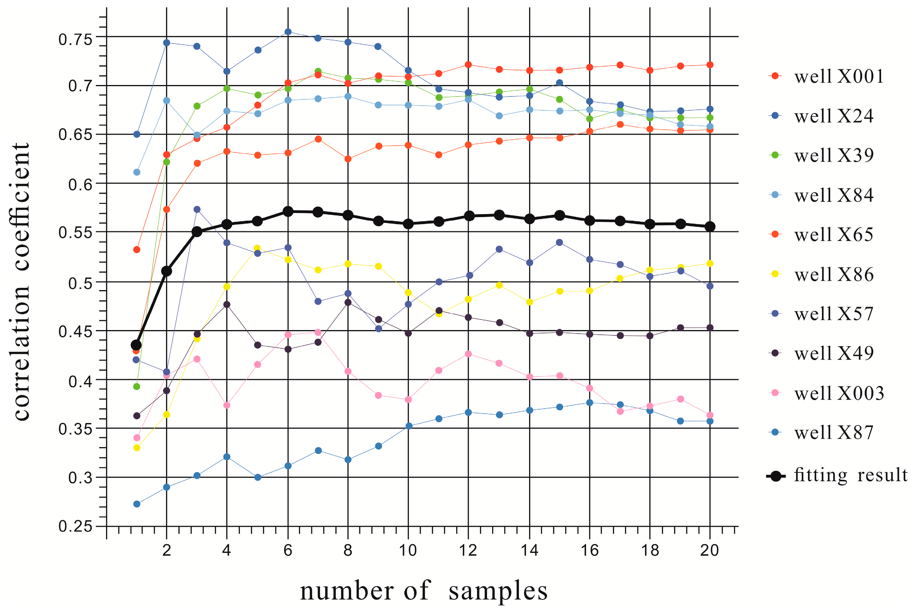
The above process is illustrated in Figure 2, in which the horizontal axis represents the number of sample points involved in the calculation, i.e., the number of wells used in the estimation of a prediction point, and the vertical axis represents the correlation coefficient. The correlation coefficient is dependent on the frequency range of the seismic data selected for the inversion, and therefore, its relative changes rather than its absolute values are of more analytical importance in this study. Each curve in Figure 2 depicts how the correlation coefficient between the estimated and measured log traces at a prediction well varies as the number of sample wells increases. In particular, the black curve is the combined correlation coefficient curve, which is the main curve used to determine the effective sample size. As is shown in Figure 2, the correlation coefficient gradually increases as the number of sample wells increases from one to six. This is attributed to the fact that as the number of sample wells increases, the estimation accuracy at the prediction well continues to improve, leading to increased shape similarity between the estimated and measured log traces. When the number of sample wells exceeds six, the correlation coefficient decreases or basically remains the same, indicating that the use of more sample wells is not always beneficial in increasing the prediction accuracy. That is, the seismic waveforms at the excess sample wells have a low correlation with that at the prediction well (because they are not in the same sedimentary facies as the prediction well), and thus, they do not contribute to the estimation of the log traces at the prediction well and may even lead to an increase in the estimation error. As was discussed above, it is clear that the number of samples at the turning point of the fitted curve is the effective sample size that will lead to the highest correlation between the estimated and actual log traces.

The effective sample size is closely related to the spatial variation characteristics of the reservoirs in the actual prospecting areas, but it depends on the lateral changes and vertical structure complexity of the reservoirs. In areas with stable deposits, similar reservoir structures and similar seismic response characteristics exist at different locations. Higher structural similarity among known samples leads to a larger effective sample size and thereby a lower screening threshold for similar seismic waveforms, which in turn leads to a smaller number of seismic facies. That is, the fewer the seismic facies, the smaller the spatial variation to be modeled, and the stronger the continuity of the inversion results. In contrast, the faster the lateral changes in the reservoir and the more complex the reservoir structure, the worse the regularity of the seismic facies. The structural similarity among the known samples becomes lower as the regularity of the seismic facies decreases, which in turn decreases the effective sample size, leading to a higher screening threshold for similar seismic waveforms and thereby a larger number of seismic facies. That is, the larger the number of seismic facies, the larger the spatial variation to be modeled, the worse the continuity of the inversion results, and the more accurate the delineation of the real distribution characteristics of the reservoirs.

2.3. Determination of the Optimal Cutoff Frequency

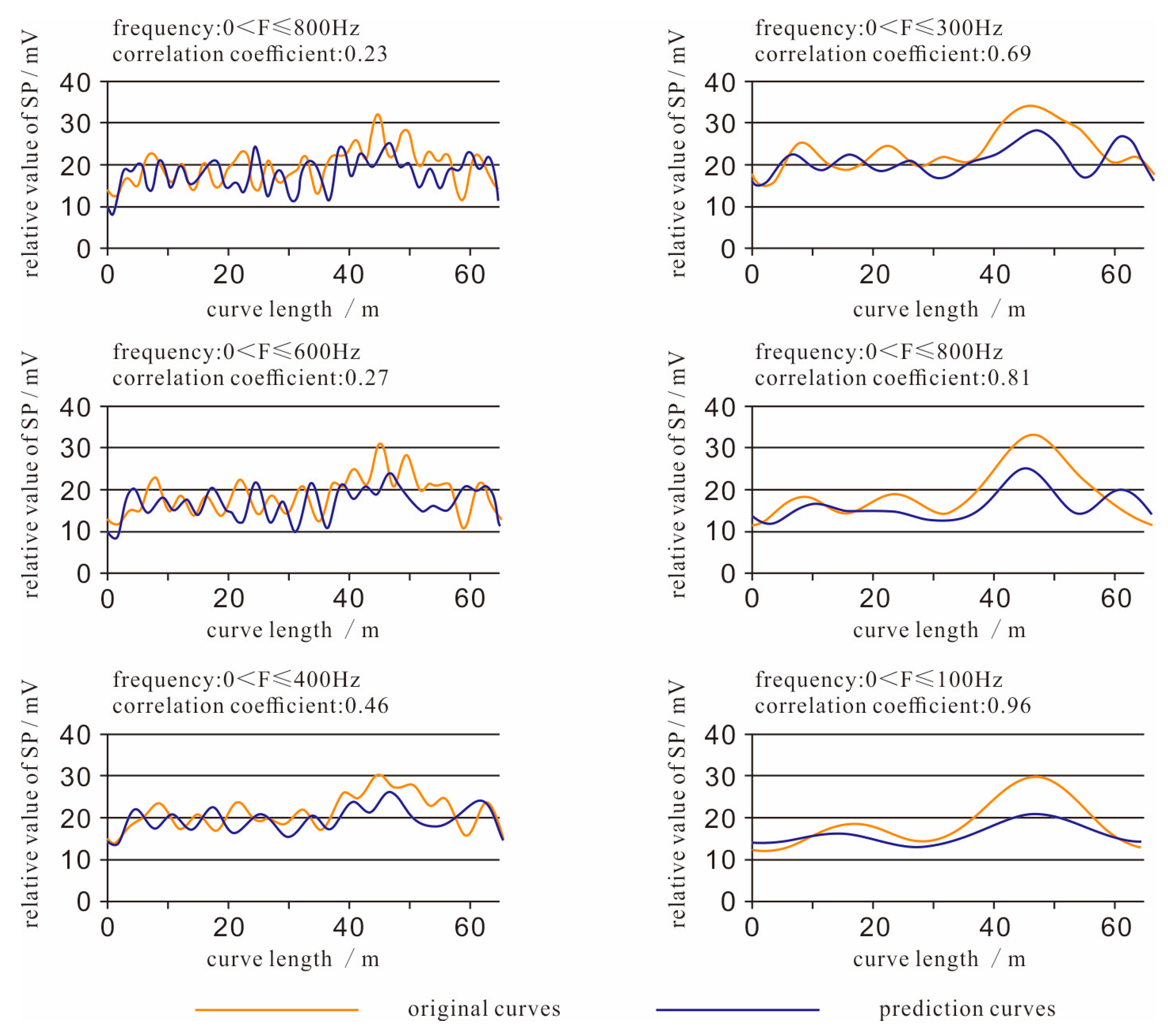
It has been observed that the correlation between an FCMCMC algorithm-predicted curve and the measured curve is frequency-dependent, suggesting that the accuracy of the predicted curve is frequency-dependent. Therefore, it is necessary to determine the optimal cutoff frequency to make the prediction results have the greatest correlation. As is shown in Figure 3, the correlation coefficient between the predicted and measured curves is 0.96 when the frequency components are between 0 and 100 Hz (but not equal to 0). When the frequency is greater than 0 but less than or equal to 200 Hz, the correlation coefficient is 0.81; when the frequency is greater than 0 but less than or equal to 300 Hz, the correlation coefficient is 0.69; when the frequency is greater than 0 but less than or equal to 400 Hz, the correlation coefficient is 0.46; when the frequency is greater than 0 but less than or equal to 600 Hz, the correlation coefficient is 0.27; and when the frequency is greater than 0 but less than or equal to 800 Hz, the correlation coefficient is only 0.23. Therefore, the smaller the frequency range, the higher the similarity between the predicted and measured curves, i.e., the higher the reliability of the prediction. As the frequency increases, the correlation between the predicted and measured curves gradually becomes lower, suggesting an increasing stochasticity in the high-frequency components of the curve and thereby a gradual degradation of their reliability. Therefore, it is important to identify the optimal cutoff frequency that can be used to minimize the uncertainty of the prediction results while meeting the resolution requirements for reservoir prediction.

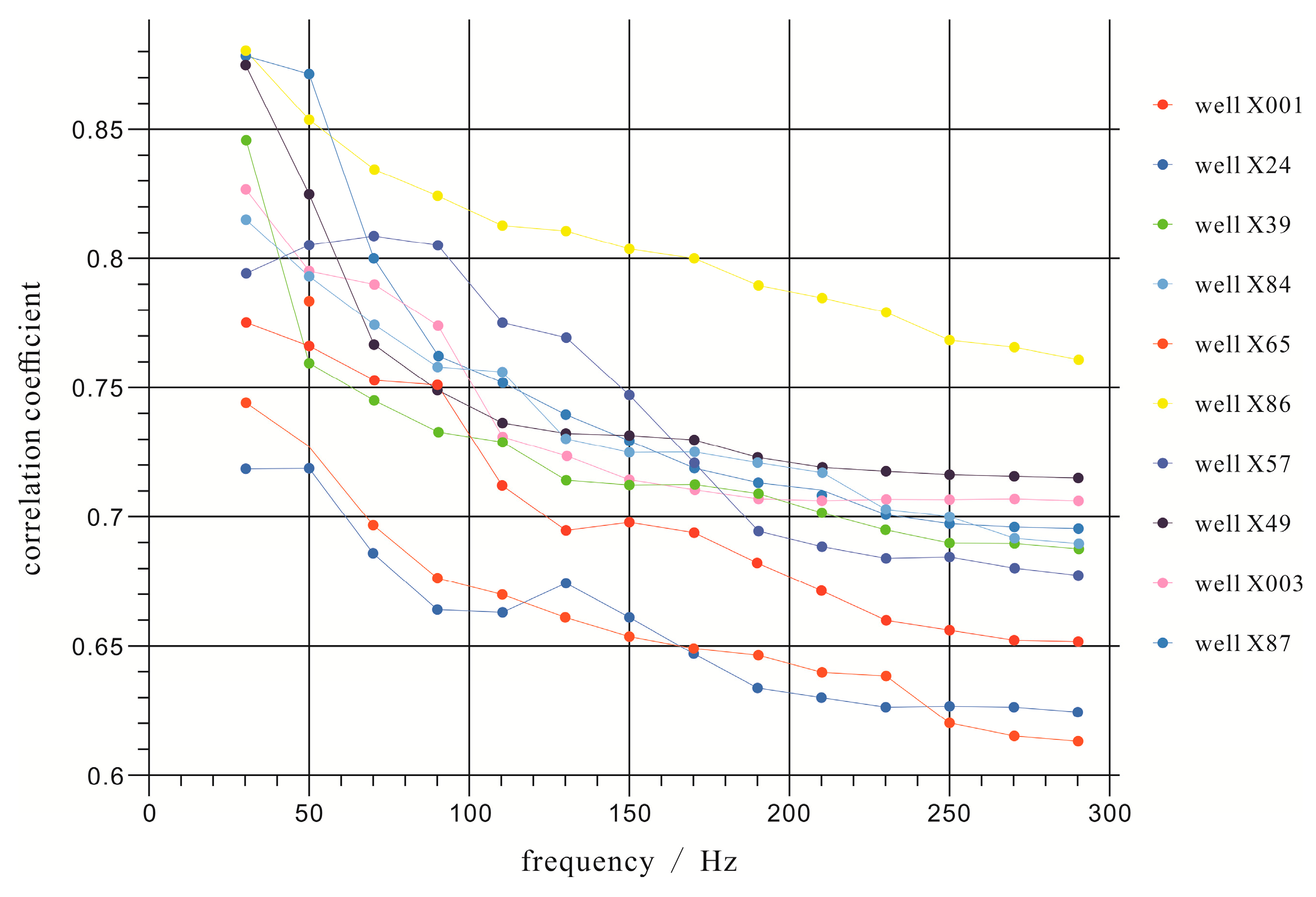
The optimal cutoff frequency can be determined as follows. (1) A known sample well is selected and assumed to be the prediction well, for which the prediction is performed using the previously determined effective sample size (see Section 2.2.2), followed by the application of frequency filters to the predicted and measured curves; the calculation of the correlation coefficients between the two curves at different cutoff frequencies; and the plotting of the curves of the correlation coefficients vs. the cutoff frequencies (Figure 4). In Figure 4, the horizontal axis represents the different cutoff frequencies, and the vertical axis represents the correlation coefficient between the predicted and the measured curves. As is shown in Figure 4, the correlation coefficients decrease with the increasing cutoff frequencies, meaning a gradual increase in the error of the predicted curve relative to the measured curve as the cutoff frequency increases. The curves of the correlation coefficients vs. the cutoff frequencies gradually level off after the cutoff frequency exceeds 230 Hz, suggesting a high stochasticity and thereby a high uncertainty in the prediction results for this frequency range. Therefore, the optimal cutoff frequency was determined to be 230 Hz.

It should be noted that the optimal cutoff frequency is strongly dependent on the effective sample size, and thereby, it should be determined only after the effective sample size is determined. In addition, when determining the optimal cutoff frequency, it is necessary to consider the minimum reservoir thickness to be identified. When there is no requirement for the identification of thin reservoirs, the SP inversion may be performed at a lower cutoff frequency rather than at the optimal cutoff frequency, in order to increase the certainty of the inversion results, whereas the SP inversion can be performed at a higher cutoff frequency rather than at the optimal cutoff frequency to meet the high resolution requirement for predicting a small reservoir thickness; however, this may increase the stochasticity of the inversion results.

2.4. FCMCMC Algorithm-Based Geostatistical Inversion

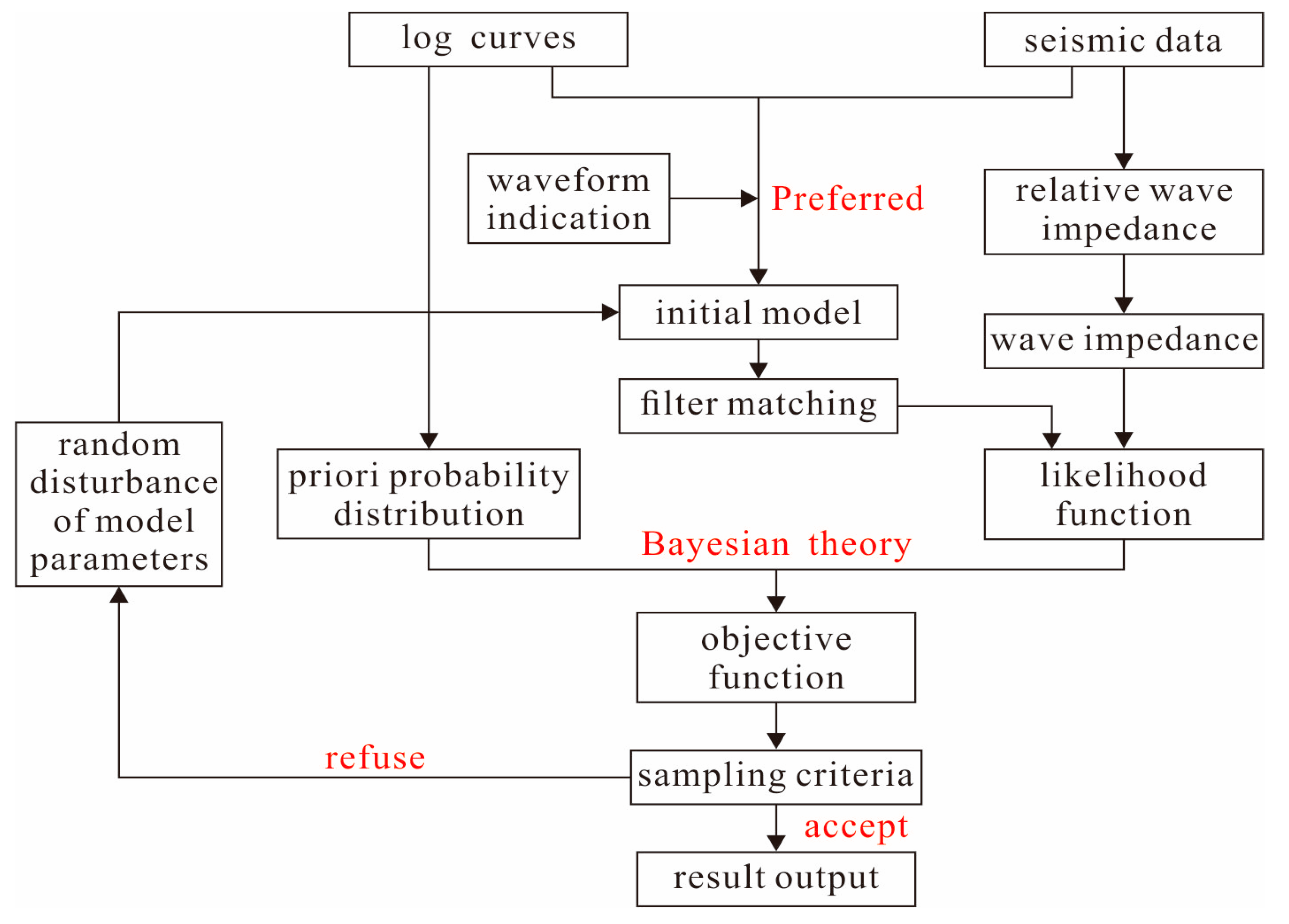
The FCMCMC algorithm-based geostatistical inversion involves the following five steps (Figure 5). (1) A tectonic model of the target layer is established based on the tectonic interpretation. (2) The seismic waveform characteristics of the seismic traces near the completed wells in the target layer are analyzed, followed by the evaluation of the correlation between the seismic waveform near the prediction well and those near the completed wells under the constraints of the tectonic model; the selection of the completed wells whose seismic waveforms have the highest correlation with that near the prediction well; and the use of the selected completed wells as sample wells to construct the initial acoustic impedance model. (3) The high-frequency components of the acoustic impedances of the sample wells in the target layer are extracted through spectral decomposition, followed by an analysis of the common structural features of the high-frequency components and the identification and retaining of the effective components within the stable bandwidth. (4) The high-frequency components of the initial model are optimized in the Bayesian framework, followed by a comparison of the predicted acoustic impedance with the measured acoustic impedance within the effective seismic bandwidth; the retaining of the solutions with errors within an accepted range; and the repetition of the simulation to ensure that the medium-frequency components of the stochastic solutions are always consistent with the seismic data and that the deterministic structural components of the samples are retained. (5) Finally, the inversion results are output.

3. Results

3.1. Lithology and Pore Structures

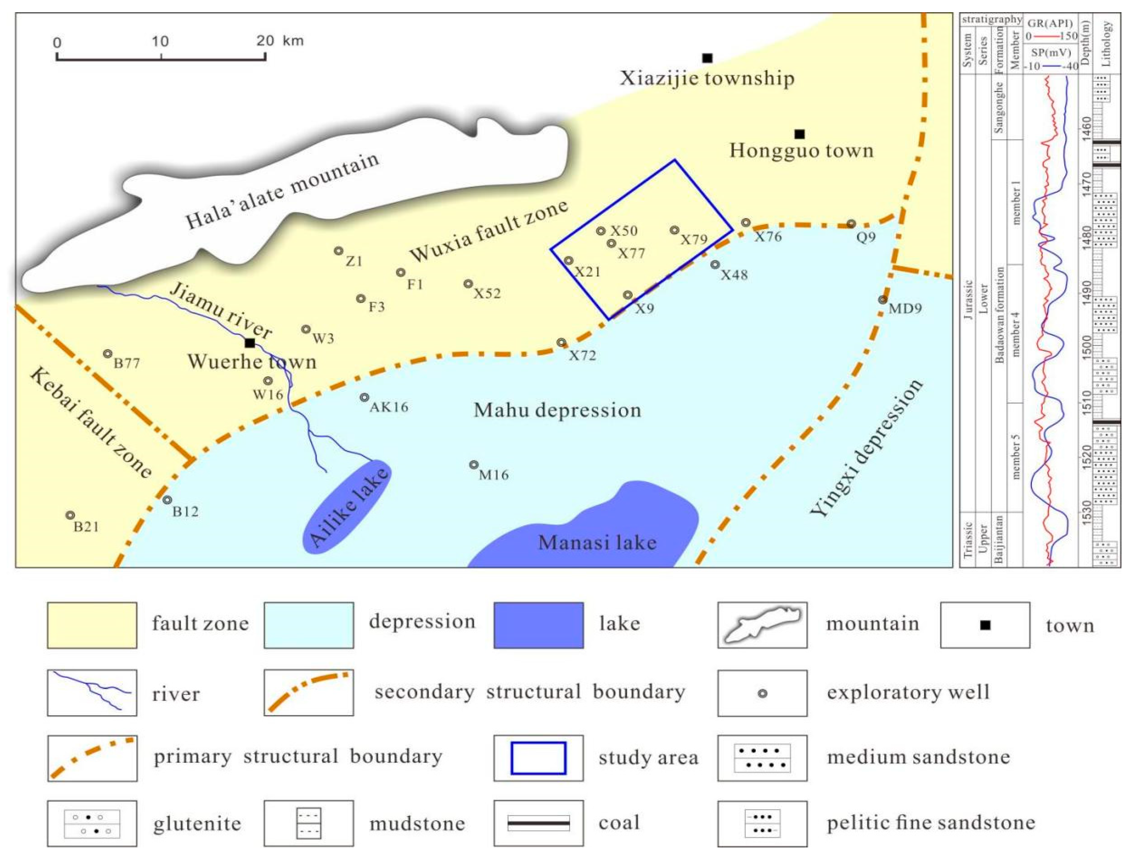
The Xiazijie Oilfield is located in the eastern part of the Wuxia fault zone on the northwestern margin of the Junggar Basin. Administratively, it is located in the Mongolian Autonomous County of Hoboksar, Xinjiang Uygur Autonomous Region. The study area is about 32 km long from east to west and 18 km wide from north to south. It is bounded by the Hala’alate Mountains to the north, the Wuerhe Oilfield to the west, the Hongqiba region to the east, and the Mahu Depression to the south, and it is the largest hydrocarbon-bearing depression on the northwestern margin (Figure 6). The left side of Figure 6 shows the structural and geographical location of the work area, as detailed in the legend. The left side of Figure 6 shows the comprehensive stratigraphic histogram of the work area. The borehole log data indicate that the stratigraphy from bottom to top is composed of the Triassic Baikouquan (T₁b), Karamay (T₁k), and Baijiantan (T₃b) formations; the Jurassic Badaowan (J₁b), Sangonghe (J₁s), Xishangyao (J₂x), Toutunhe (J₂t), and Qigu (J₃q) formations; and the Cretaceous Tugulu Group (K₁tg). In particular, there are regional unconformities between the Cretaceous strata and the Jurassic strata and between the Jurassic strata and the Triassic strata. In the target layer, the Badaowan Formation is located in the lowest part of the Jurassic strata, and it directly overlies the Triassic strata, forming an angular unconformity with the Triassic strata. Based on the lithology and electrical properties, the Badaowan Formation can be further divided into three sandstone formations, J₁b¹, J₁b⁴, and J₁b⁵; while the J₁b² and J₁b³ sandstone formations are missing, with a parallel unconformity between J₁b¹ and J₁b⁴. The current tectonic framework of the study area was mainly formed at the end of the Indosinian movement. The tectonic pattern of the target layer has the following characteristics. (1) The layer generally dips from northwest to southeast. (2) It contains a large-scale thrust fault zone in the north, which gradually thrusts southward. (3) The entire southern part is a monocline, with a fault-nose structure and a nose-like structure in local areas. The Badaowan Formation mainly contains braided river sediments sourced from the Hala’alate Mountains to the northeast. The facies are mainly composed of channel subfacies and floodplain subfacies, and the channel subfacies mainly include channel bar deposit and riverbed deposit microfacies. There are two modes of the vertical stacking of sedimentary facies. One is to develop the sedimentation model of riverbed deposit, channel bar deposit, and floodplain from bottom to top; the lithology is characterized by thick sandstone with thin mudstone. The other is the combination of riverbed deposit sediment and floodplain; it is shown as the interbed of coarse-grained glutenite and mudstone. The river channels exhibit a strip-shaped form and extend from the provenance area, while the channel bars are vertical and are mostly distributed in a beaded form [42,43]. The reservoirs are mainly composed of channel bar sand bodies and riverbed sand bodies, and the sand bodies are 1.5–10.8 m thick (with a mean of 6.3 m). The lithology of the Badaowan Formation in the Xiazijie Oilfield mainly includes conglomerate, glutenite, sandstone (fine sandstone, medium sandstone, and coarse sandstone), siltstone, and mudstone, with only the conglomerate, glutenite, and sandstone constituting the reservoirs.

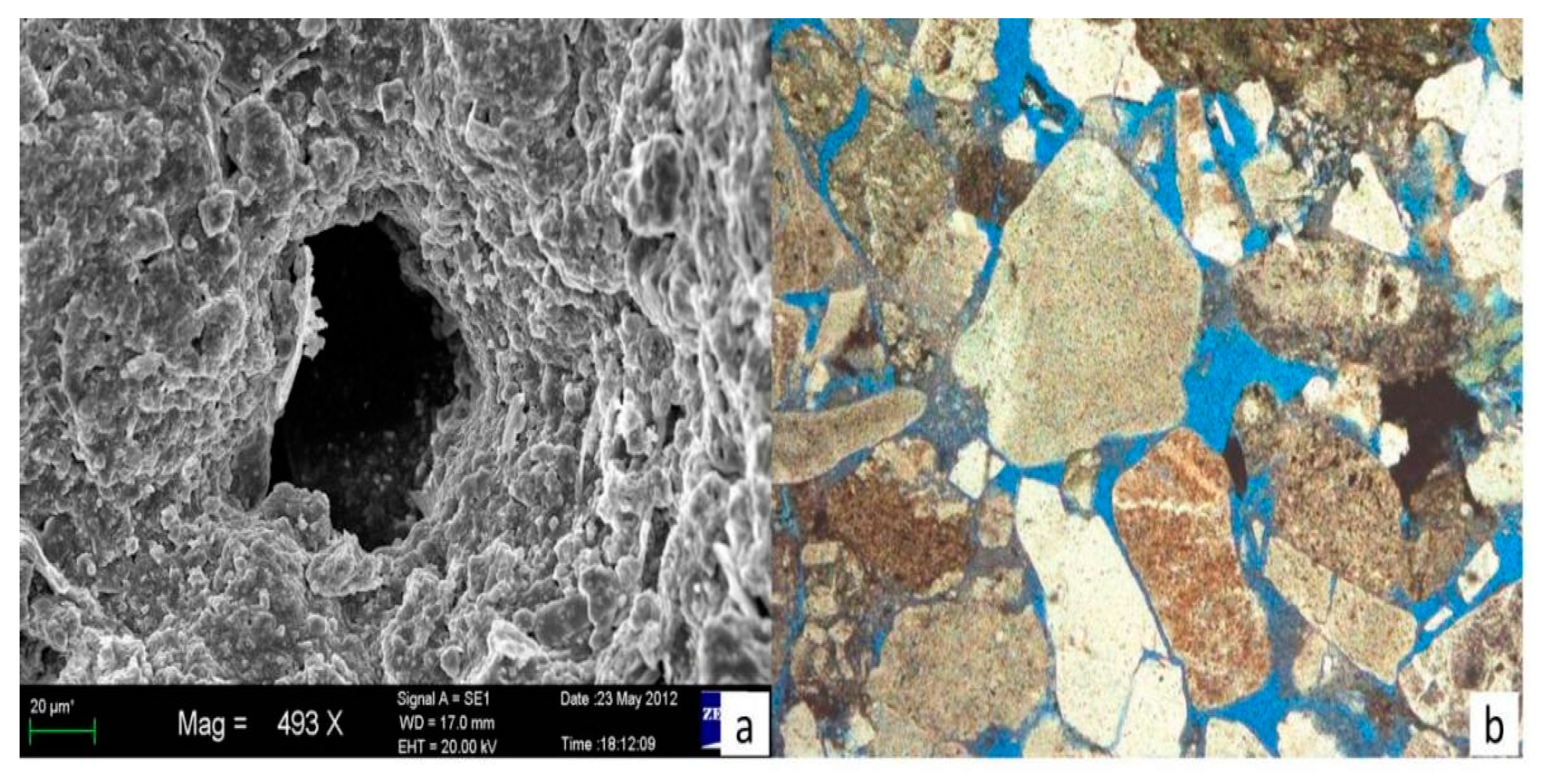
Due to their proximity to the provenance, the sediments are compositionally complex and coarse-grained, and they mostly include conglomerate and pebbly sandstone with a low maturity. They are rounded and have an angular subcircular shape. According to the analysis of the SEM data, the reservoir space of Badaowan Formation in the study area is dominated by intergranular pores, accounting for about 93.1% of the total void volume. The pores are developed, and the structure is relatively uniform (Figure 7a). The clastic particles can be seen under the cast thin slice, mostly in point line contact and stacked tightly, reflecting that the sandstone is subject to strong compaction. Although the primary intergranular pores are reduced due to the strong compaction transformation of the rock, the limit is not reached, and a large number of residual primary intergranular pores are still preserved (Figure 7b). The porosity ranges from 1.12% to 20.14%, with a mean of 15.5%. The permeability ranges from 0.16 mD to 31.14 mD, with a mean of 18.1 mD. Comprehensive evaluation has revealed that the reservoirs in the Badaowan Formation in the study area are medium-porosity, low-permeability reservoirs.

3.2. Electrical Characteristic

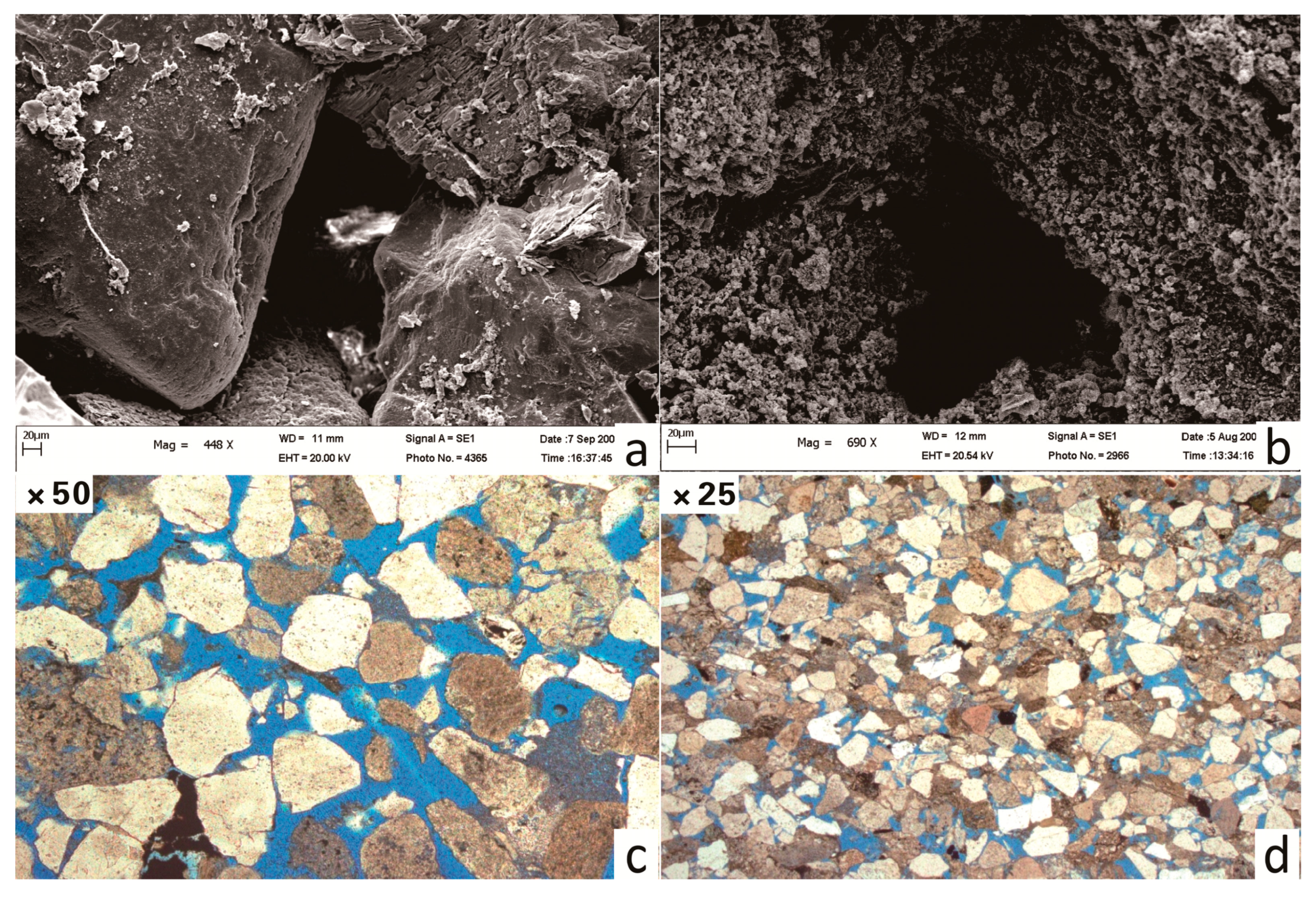
In order to strictly implement the lithological boundary between reservoir and non-reservoir and to determine the reliability of fine sandstone as the lower limit of reservoir, we carried out SEM and cast thin slice experimental analysis on medium-grained sandstone and fine sandstone. Figure 8a,b are SEM images of sandstone in wells X84 and X003. According to these two figures, it can be seen that the intergranular pores of the medium-grained and fine sandstone are developed. Figure 8c shows the cast thin slice of medium-grained sandstone at a depth of 1178.58 m in well X84. It can be seen that the remaining intergranular pores are well developed and well connected. Figure 8d shows the cast thin slice of fine sandstone at a depth of 1045.51 m in well X003. It can be seen that the remaining intergranular pores and primary intergranular pores are well developed. However, through comparison, it can be seen that the pore size and connectivity of medium-grained sandstone are better than those of fine sandstone [44,45].

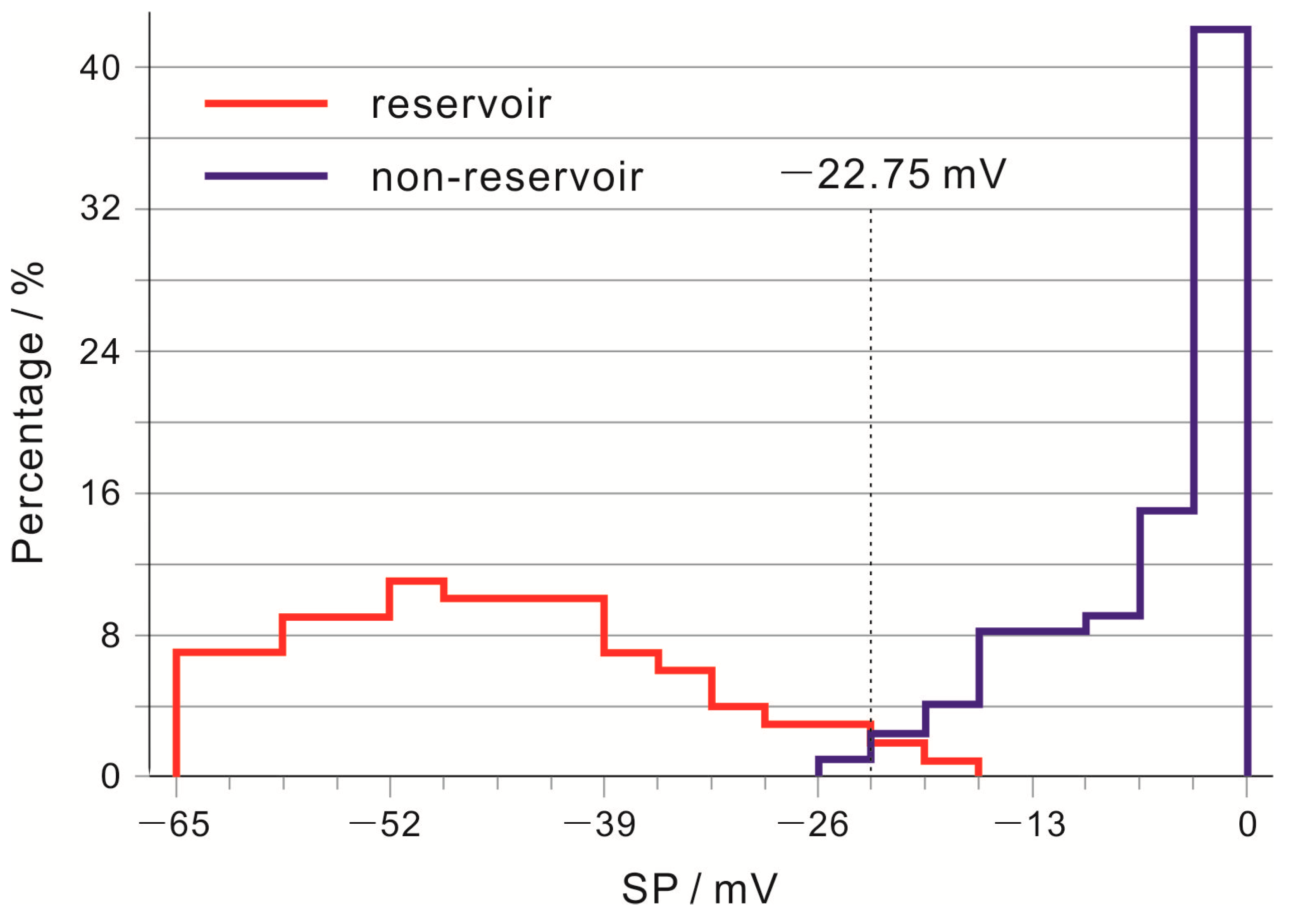
Preliminary analysis of the core and log data revealed that the p-wave impedance, acoustic transit time, and density failed to distinguish between reservoirs and non-reservoirs, thereby making it impossible to use acoustic inversion to predict the distribution of the reservoir. In addition, the natural gamma, resistivity, and compensated neutron logs also failed to distinguish between the reservoirs and non-reservoirs, with the spontaneous potential logging (SP) being the most sensitive to the reservoirs. As the value of the SP curve is relative, the abnormal value removal, baseline correction, and normalization of the spontaneous potential curve were carried out before rock physics and inversion research. Then, petrophysical analysis was performed based on the core data of the Badaowan Formation in the Xiazijie Oilfield and the corresponding processed log data for the SP. As is shown by the histograms of the SP (Figure 9), the reservoirs and non-reservoirs are distinct in terms of their SP values, with little overlap. The cutoff value of the SP between the reservoirs and non-reservoirs is less than −22.75 mV, that is, SP > −22.75 mV indicates the presence of mudstone and argillaceous siltstone (i.e., non-reservoirs), while SP < −22.75 mV indicates the presence of glutenite, conglomerate, and sandstone (i.e., reservoirs).

3.3. Inversion and Analysis

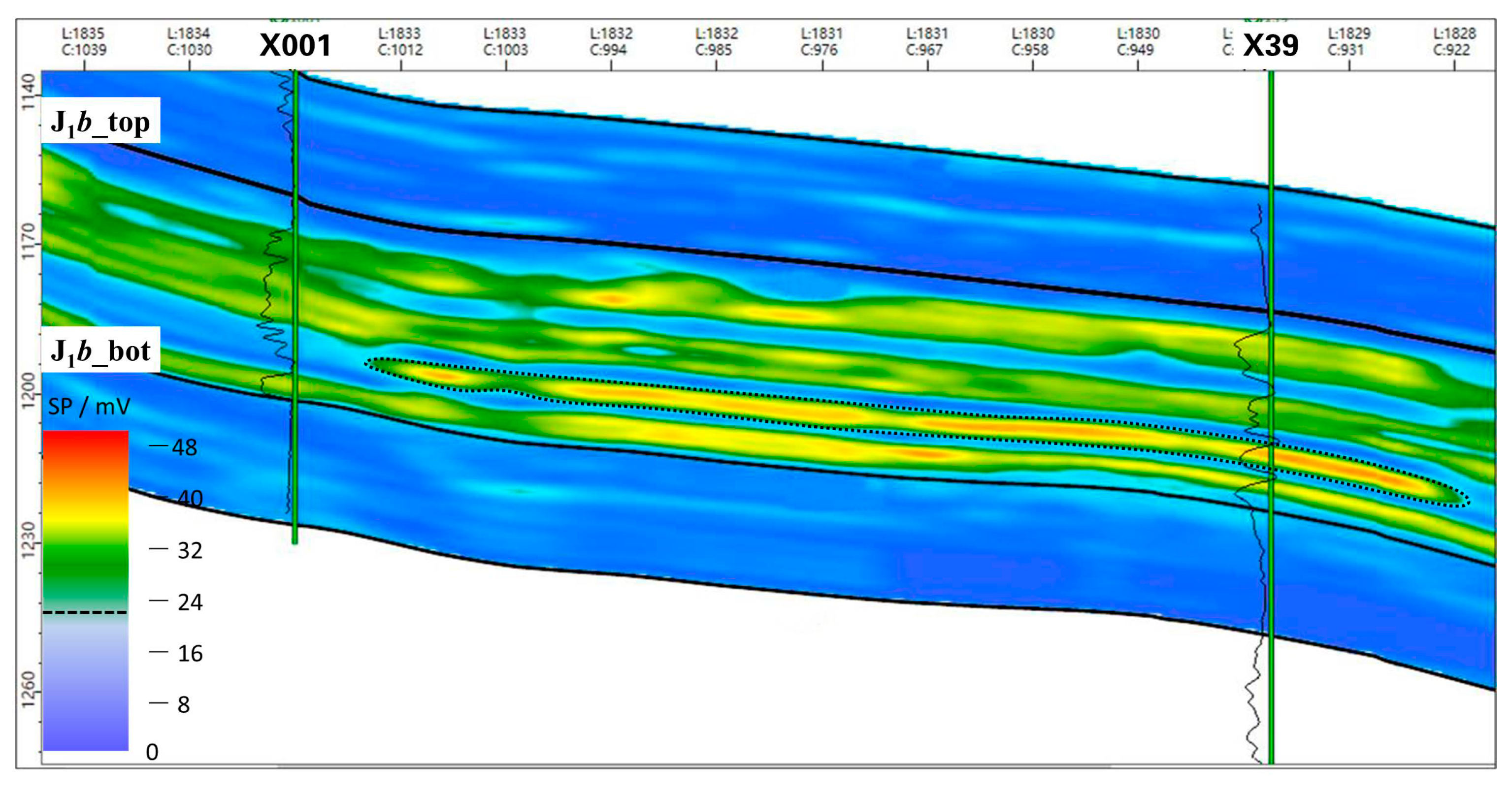
The above methodology was applied to the prediction of the distribution characteristics of the sand bodies in the channel bars of the braided river sediments in the Jurassic Badaowan Formation in the Xiazijie Oilfield. Figure 10 shows the SP profile that continuously runs through wells X001–X39. The black line labeled with a name in the figure represents the top and bottom of the Badaowan Formation; the black line without a name represents the top and bottom range of the inversion result; the brown line represents the well trajectory; the top of the well trajectory is the name of the wells; and the SP curves are next to the well trajectory. The petrophysical analysis revealed that SP < −22.75 mV indicated the presence of glutenite, conglomerate, and sandstone reservoirs; so, the cutoff SP was set as −22.75 mV in this study. The blue background in the profile represents the non-reservoirs, while the red and yellow represent the reservoirs. The curves present the processed SP logs for the corresponding wells. A total of seven verification wells were designed for this inversion, and six wells were consistent with the inversion results, with a coincidence rate of 85.7%. Several observations can be made from Figure 10.

• As can be seen from the profile of the inverted SP, the inversion results are completely consistent with the interpretation results of the well log data, and the distinctions of the reservoirs and non-reservoirs are clearly delineated.
• Not only the reservoirs but also the mudstone interbeds are clearly delineated in the profile.
• The sand body enclosed by the dashed line is the target sand body, with a maximum thickness of 6 m, and its distribution and pinch-out are clearly delineated.
• The target body is mainly distributed around well X39, and it pinches out near well X001, which is fully consistent with the log data from the completed wells.

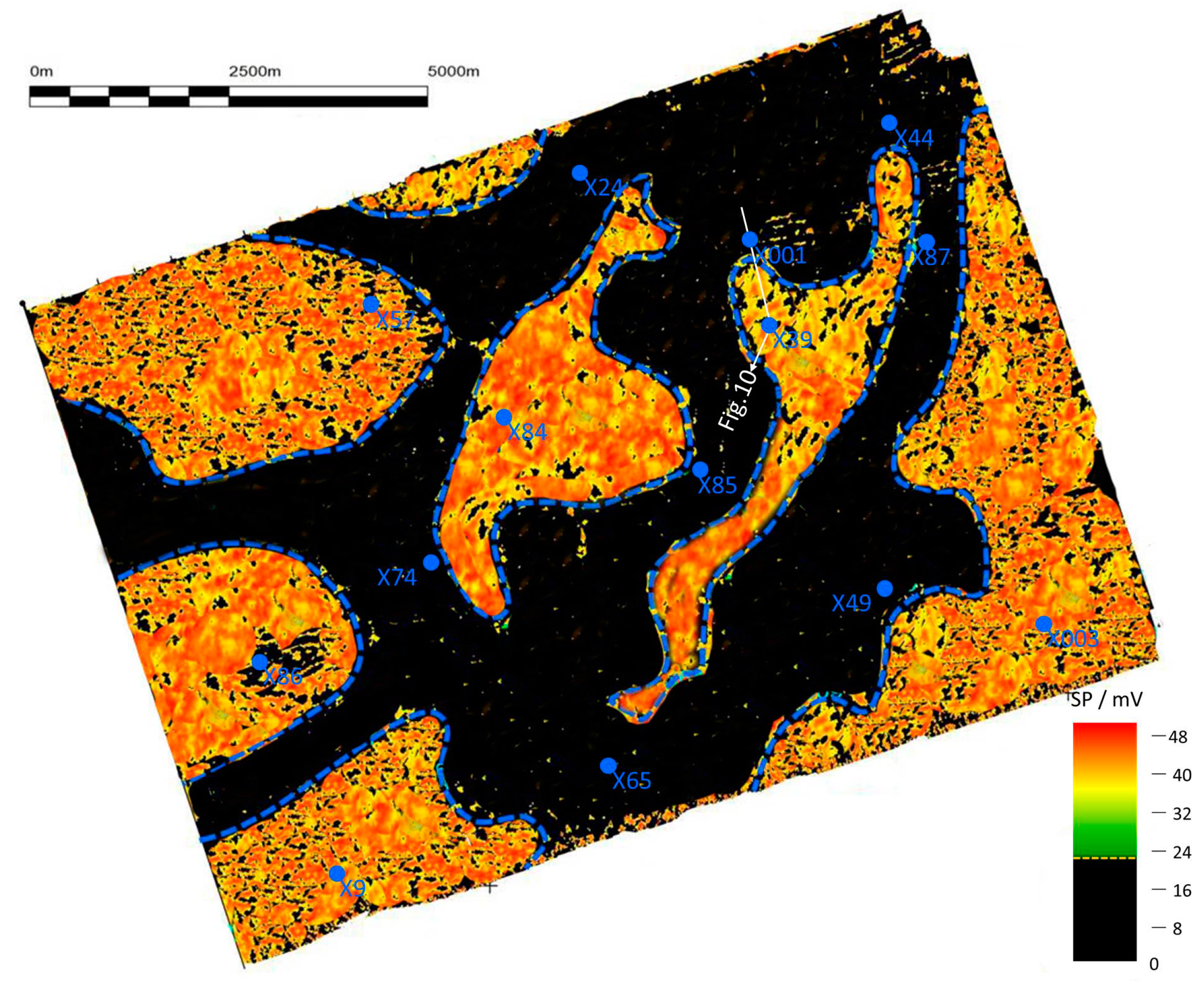
Figure 11 shows the horizontal distribution of the SP of the Jurassic Badaowan Formation in the study area. The braided river channels and the channel bars are shown in black and yellow–red, respectively, to clearly reveal the distribution relationship between the river channels and the channel bars. The source materials in the study area are derived from the provenance area to the northeast. The braided river channels exhibit a broad, strip-shaped form, extending from the NE to the SW. In addition, a number of vertical bars formed along the extension direction of the channels, mainly consisting of six large, relatively independent bars that are mutually separated by the channels, namely bars X39, X84, X57, X9, X003, and X86. These observations are consistent with the well log data and are also consistent with the known geological setting of the study area, fully confirming the reliability of the prediction results and thereby the soundness of the proposed technique.

4. Discussion

The method described in this paper not only retains the advantages of traditional geostatistics inversion, but also strengthens the constraint function of sedimentary facies in the inversion process. The theory and practices demonstrate that this technique is suitable for the seismic prediction of various complex reservoirs, especially thin reservoirs with significant variations in one or more lithological parameters [46,47,48]. This technique not only provides high-accuracy inversion results, but it also allows a quantitative evaluation of the reliability of the results in different frequency ranges. Finally, this inversion technique does not have a rigorous requirement concerning the number and horizontal distribution of the completed used wells, thereby making it suitable for use in all of the stages of oil and gas exploration and development. However, it should be noted that any single seismic technology has limitations and uncertainties. Therefore, when using this technology, attention should be paid to the joint application with a variety of other seismic technologies and the maximum combination of geological prior information to improve the reliability of the reservoir prediction.

In addition, this method also has the same shortcomings as other geostatistics inversion methods. It requires a large number of statistical samples, that is, completed wells. When there are few wells, the inversion effect is poor. Moreover, this method is purely mathematical and has no physical or geological significance. Although this paper has improved this problem to a certain extent, it still cannot be completely solved. When the quality of the seismic data is poor and when the seismic waveform cannot reflect the distribution characteristics of the sedimentary facies, the application of this method will be limited, and the reliability of the inversion results will be affected.

5. Conclusions

In this study, a geostatistical inversion technique was developed based on a facies-constrained MCMC algorithm, which leveraged the lateral changes in the seismic waveforms as geologically relevant information to drive the construction of a variogram and the selection of the statistical sampling. At present, the idea of using seismic waveforms to represent geological significance to constrain the inversion process is a new field. This method of using seismic waveforms to drive sample optimization has not been discussed by scholars. Geostatistics inversion based on this method is also an innovative idea. This technique overcomes the traditional problem of geostatistical inversion techniques, namely the failure to accurately delineate the sedimentary characteristics. In addition, it expands the application scope of seismic inversion, while improving the resolution of the inversion results, thereby truly achieving facies-constrained geostatistical inversion. This method proved to be feasible and accurate in the prediction of the braided river channel and core beach sand body of the Badaowan Formation in Xiazijie oilfield, Junggar Basin, China; moreover, this method can be implemented repeatedly. This research idea is not limited to usage in geostatistics inversion based on the CMMC algorithm; we are trying to extend this research idea of taking the seismic waveform as a geological constraint to other geostatistics inversion algorithms, even including nonlinear inversion such as neural network inversion, which should be of positive significance for improving the practicability of various inversion technologies.

References

- Gao, J.; Huang, G.; Ji, M. Seismic phase-controlled nonlinear inversion of a carbonate reservoir. Geophys. Prospect. Pet. 2020, 59, 396–403. [Google Scholar]
- Guo, L.L.; Zhou, D.W.; Zhang, D.M. Deformation and failure of surrounding rockof a roadway subjected to mining-induced stresses. J. Min. Strat. Control Eng. 2021, 3, 023038. [Google Scholar]
- Jia, C.; Zou, C.; Yang, Z. Significant progress of continental petroleum geology theory in basins of Central and Western China. Pet. Explor. Dev. 2018, 45, 546–560. [Google Scholar] [CrossRef]
- Chen, H.; Yin, X.; Gao, J. Seismic inversion for underground fractures detection based on effective anisotropy and fluid substitution. Sci. China Earth Sci. 2015, 58, 805–814. [Google Scholar] [CrossRef]
- Djebbar, T.; Erle, C. Petrophysics: Theory and Practice of Measuring Reservoir Rock and Fluid Transport Properties, 3rd ed.; Petroleum Industry Press: Beijing, China, 2016; pp. 1–17. [Google Scholar]
- Du, J.; Hu, S.; Pang, Z. The types, potentials and prospects of continental shale oil in China. China Pet. Explor. 2019, 24, 560–568. [Google Scholar]
- Chen, Y.; Bi, J.; Qiu, X. A method of seismic meme inversion and its application. Pet. Explor. Dev. 2020, 47, 1149–1158. [Google Scholar] [CrossRef]
- Huang, Z.; Gan, L.; Dai, X. Key parameter optimization and analysis of stochastic seismic inversion. Appl. Geophys. 2012, 9, 49–56. [Google Scholar] [CrossRef]
- Han, C.; Lin, C.; Ren, L. Application of seismic waveform inversion in Es4s beach-bar sandstone in Wangjiagang area, Dongying Depression. J. China Univ. Pet. Ed. Nat. Sci. 2017, 41, 60–69. [Google Scholar]
- Li, Q.; He, J.; Li, Z. Identification of sand body based on seismic high resolution 3D nonlinear inversion in Moxizhuang, Junggar basin, China. J. Chengdu Univ. Technol. Sci. Technol. Ed. 2017, 44, 727–737. [Google Scholar]
- Li, Q.; Luo, Y.; Zhang, S. High-resolution Bayesian sequential stochastic inversion. Oil Geophys. Prospect. 2020, 55, 389–397. [Google Scholar]
- Bouchaala, F.; Ali, M.Y.; Matsushima, J.; Bouzidi, Y.; Jouini, M.S.; Takougang, E.M.; Mohamed, A.A. Estimation of seismic wave attenuation from 3D seismic data: A case study of OBC data acquired in an offshore oilfield. Energies 2022, 15, 534. [Google Scholar] [CrossRef]
- Matsushima, J.; Ali, M.Y.; Bouchaala, F. A novel method for separating intrinsic and scattering attenuation for zero-offset vertical seismic profiling data. Geophys. J. Int. 2017, 211, 1655–1668. [Google Scholar] [CrossRef]
- Adam, L.; Batzle, M.; Lewallen, K.T.; van Wijk, K. Seismic wave attenuation in carbonates. J. Geophys. Res. Solid Earth 2009, 114. [Google Scholar] [CrossRef]
- Ahmad, Q.A.; Wu, G.; Jianlu, W. Computation of wave attenuation and dispersion, by using quasi-static finite difference modeling method in frequency domain. Ann. Geophys. 2017, 60, S0664. [Google Scholar]
- Lan, S.R.; Song, D.Z.; Li, Z.L. Experimental study on acoustic emission characteristics of fault slip process based on damage factor. J. Min. Strat. Control Eng. 2021, 3, 033024. [Google Scholar]
- Li, J.; Li, H.; Yang, C.; Wu, Y.J.; Gao, Z.; Jiang, S.L. Geological characteristics and controlling factors of deep shale gas enrichment of the Wufeng-Longmaxi Formation in the southern Sichuan Basin, China. Lithosphere 2022, 2022, 4737801. [Google Scholar] [CrossRef]
- Li, H.; Zhou, J.L.; Mou, X.Y.; Guo, H.X.; Wang, X.X.; An, H.Y.; Mo, Q.W.; Long, H.Y.; Dang, C.X.; Wu, J.F.; et al. Pore structure and fractal characteristics of the marine shale of the Longmaxi Formation in the Changning Area, Southern Sichuan Basin, China. Front. Earth Sci. 2022, 10, 1018274. [Google Scholar] [CrossRef]
- Li, H. Research progress on evaluation methods and factors influencing shale brittleness: A review. Energy Rep. 2022, 8, 4344–4358. [Google Scholar] [CrossRef]
- Fan, C.H.; Xie, H.B.; Li, H.; Zhao, S.X.; Shi, X.C.; Liu, J.F.; Meng, L.F.; Hu, J.; Lian, C.B. Complicated fault characterization and its influence on shale gas preservation in the southern margin of the Sichuan Basin, China. Lithosphere 2022, 2022, 8035106. [Google Scholar] [CrossRef]
- Wang, J.; Wang, X.L. Seepage characteristic and fracture development of protected seam caused by mining protecting strata. J. Min. Strat. Control Eng. 2021, 3, 033511. [Google Scholar]
- Li, H.; Tang, H.M.; Qin, Q.R.; Zhou, J.L.; Qin, Z.J.; Fan, C.H.; Su, P.D.; Wang, Q.; Zhong, C. Characteristics, formation periods and genetic mechanisms of tectonic fractures in the tight gas sandstones reservoir: A case study of Xujiahe Formation in YB area, Sichuan Basin, China. J. Petrol. Sci. Eng. 2019, 178, 723–735. [Google Scholar] [CrossRef]
- Zhang, B.; Shen, B.; Zhang, J. Experimental study of edge-opened cracks propagation in rock-like materials. J. Min. Strat. Control. Eng. 2020, 2, 033035. [Google Scholar]
- Liu, J.; Shi, L.; Dong, N. The processing technique of improving the resolution for the thin hydrocarbon reservoir with coal seam. Geophys. Prospect. Pet. 2017, 56, 216–221. [Google Scholar]
- Gao, F.Q. Influence of hydraulic fracturing of strong roof on mining-induced stress insight from numerical simulation. J. Min. Strat. Control Eng. 2021, 3, 023032. [Google Scholar]
- Mu, L.; Ji, Z. Technology progress and development directions of Petrochina overseas oil and gas exploration. Pet. Explor. Dev. 2019, 46, 1027–1036. [Google Scholar] [CrossRef]
- Pan, X.; Zhang, G.; Yin, X. Probabilistic seismic inversion for reservoir fracture and petrophysical parameters driven by rock-physics models. Chin. J. Geophys. 2018, 61, 683–696. [Google Scholar]
- Todorov, V.; Dimov, I. Efficient Stochastic Approaches for Multidimensional Integrals in Bayesian Statistics. In Large-Scale Scientific Computing; Lirkov, I., Margenov, S., Eds.; LSSC 2019; Lecture Notes in Computer Science; Springer: Cham, Switzerland, 2020; Volume 11958. [Google Scholar]
- Yousef, M.M.; Hassan, A.S.; Al-Nefaie, A.H.; Almetwally, E.M.; Almongy, H.M. Bayesian Estimation Using MCMC Method of System Reliability for Inverted Topp–Leone Distribution Based on Ranked Set Sampling. Mathematics 2022, 10, 3122. [Google Scholar] [CrossRef]
- Raveendran, N.; Sofronov, G. A Markov Chain Monte Carlo Algorithm for Spatial Segmentation. Information 2021, 12, 58. [Google Scholar] [CrossRef]
- Dimov, I.; Maire, S.; Todorov, V. An unbiased Monte Carlo method to solve linear Volterra equations of the second kind. Neural Comput. Appl. 2022, 34, 1527–1540. [Google Scholar] [CrossRef]
- Li, L.; Li, S.J. Evolution rule of overlying strata structure in repeat mining of shallow close distance seams based on Schwarz alternating procedure. J. Min. Strat. Control Eng. 2021, 3, 023515. [Google Scholar]
- Liu, X.; Li, J.; Chen, X. A stochastic inversion method integrating multi-point geostatistics and sequential Gaussian simulation. Chin. J. Geophys. 2018, 61, 2998–3007. [Google Scholar]
- Sun, S.; Zhang, T. A 6M digital twin for modeling and simulation in subsurface reservoirs. Adv. Geo-Energy Res. 2020, 4, 349–351. [Google Scholar] [CrossRef]
- Cai, J.; Hajibeygi, H.; Yao, J. Advances in porous media science and engineering from InterPore2020 perspective. Adv. Geo-Energy Res. 2020, 4, 352–355. [Google Scholar] [CrossRef]
- Baouche, R.; Wood, D. Characterization and estimation of gas-bearing properties of Devonian coals using well log data from five Illizi Basin wells (Algeria). Adv. Geo-Energy Res. 2020, 4, 356–371. [Google Scholar] [CrossRef]
- Liu, X.; Lu, Y.; Lu, Y. The application of geostatistical inversion in shale lithofacies prediction:a case study of the Lower Silurian Longmaxi marine shale in Fuling area in the southeast Sichuan basin, China. Mar. Geophys. Res. 2018, 39, 421–439. [Google Scholar] [CrossRef]
- Li, M.; Hou, L.; Zou, C. Geophysical Exploration Technology and Application of Lithostratigraphic Reservoir; Petroleum Industry Press: Beijing, China, 2005; pp. 1–12. [Google Scholar]
- Sun, L.; Zou, C.; Jia, A. Development characteristics and orientation of tight oil and gas in China. Pet. Explor. Dev. 2019, 46, 1015–1026. [Google Scholar] [CrossRef]
- Yang, J.X.; Luo, M.K.; Zhang, X.W.; Huang, N. Mechanical properties and fatigue damage evolution of granite under cyclic loading and unloading conditions. J. Min. Strat. Control Eng. 2021, 3, 033016. [Google Scholar]
- Sun, R.; Yin, X.; Wang, B. A direct estimation method for the Russell fluid factor based on stochastic seismic inversion. Chin. J. Geophys. 2016, 59, 1143–1150. [Google Scholar]
- Sun, Y. Geostatistical inversion based on Bayesian-MCMC algorithm and its applications in reservoir simulation. Prog. Geophys. 2018, 33, 724–729. [Google Scholar]
- Tan, P.; Pang, H.; Zhang, R. Experimental investigation into hydraulic fracture geometry and proppant migration characteristics for southeastern Sichuan deep shale reservoirs. J. Pet. Sci. Eng. 2020, 184, 106517. [Google Scholar] [CrossRef]
- Tan, P.; Jin, Y.; Pang, H. Hydraulic fracture vertical propagation behavior in transversely isotropic layered shale formation with transition zone using XFEM-based CZM method. Eng. Fract. Mech. 2021, 248, 107707. [Google Scholar] [CrossRef]
- Wang, P.; Li, Y.; Zhao, R. Algorithm research of post-stack MCMC lithology inversion method. Prog. Geophys. 2015, 30, 1918–1925. [Google Scholar]
- Xie, W.; Wang, Y.; Liu, X. Nonlinear joint PP-PS AVO inversion based on improved Bayesian inference and LSSVM. Appl. Geophys. 2019, 16, 750–758. [Google Scholar] [CrossRef]
- Zou, C.; Zhang, Y. New Practical Seismic Technology for Oil and Gas Exploration and Development; Petroleum Industry Press: Beijing, China, 2005; pp. 1–12. [Google Scholar]
- Zhang, G.; Pan, X.; Sun, C. PP-PS-wave prestack nonlinear inversion based on adaptive MCMC algorithm. Oil Geophys. Prospect. 2016, 51, 938–946. [Google Scholar]
Figure 1.
Schematic diagram of the sampling optimization process of the FCMCMC algorithm-based geostatistical inversion: (a) sampling optimization based on variogram ranges; (b) sampling optimization driven by seismic waveforms.
Figure 2.
Relationship between the number of sample wells and the correlation coefficient of the estimated vs. measured curves.
Figure 3.
Comparison of the estimated vs. measured curves at different cutoff frequencies.
Figure 4.
Effect of the cutoff frequency on the correlation coefficient of the relationship between the estimated and measured log traces.
Figure 5.
Flow chart of the FCMCMC algorithm-based geostatistical inversion.
Figure 6.
Geographic and tectonic map of the Xiazijie Oilfield in the Junggar Basin.
Figure 7.
(a) Scanning electron microscope of well X017 with depth of 1067.24 m; (b) casting slice of well X018 with depth of 1187.01 m.
Figure 8.
(a) Scanning electron microscope image of well X84 with depth of 1176.26 m; (b) scanning electron microscope image of well X003 with a depth of 1042.12 m; (c) cast thin section of well X84 with a depth of 1178.58 m; (d) cast thin section of well X003 with a depth of 1045.51 m.
Figure 9.
Histogram of the spontaneous potential of the Jurassic Badaowan Formation in the Xiazijie Oilfield.
Figure 10.
Profile of the inverted SP running through wells X001–X39 in the Xiazijie Oilfield.
Figure 11.
Plan view of the reservoirs of the Jurassic Badaowan Formation in the Xiazijie Oilfield.
Disclaimer/Publisher’s Note: The statements, opinions and data contained in all publications are solely those of the individual author(s) and contributor(s) and not of MDPI and/or the editor(s). MDPI and/or the editor(s) disclaim responsibility for any injury to people or property resulting from any ideas, methods, instructions or products referred to in the content. |
© 2023 by the authors. Licensee MDPI, Basel, Switzerland. This article is an open access article distributed under the terms and conditions of the Creative Commons Attribution (CC BY) license (https://creativecommons.org/licenses/by/4.0/).
Share and Cite
MDPI and ACS Style
Dong, W.; Li, Y.; Gui, Z.; Zhou, L. Theory and Application of Geostatistical Inversion: A Facies-Constrained MCMC Algorithm. Processes 2023, 11, 1335. https://doi.org/10.3390/pr11051335
AMA Style
Dong W, Li Y, Gui Z, Zhou L. Theory and Application of Geostatistical Inversion: A Facies-Constrained MCMC Algorithm. Processes. 2023; 11(5):1335. https://doi.org/10.3390/pr11051335
Chicago/Turabian StyleDong, Wenbo, Yonggen Li, Zhixian Gui, and Lei Zhou. 2023. "Theory and Application of Geostatistical Inversion: A Facies-Constrained MCMC Algorithm" Processes 11, no. 5: 1335. https://doi.org/10.3390/pr11051335
Note that from the first issue of 2016, this journal uses article numbers instead of page numbers. See further details here.