1. Introduction
Toxicity tests using experimental animals are generally performed to evaluate the toxicity of chemical substances, but there is a need to develop in silico toxicity-prediction methods from the viewpoint of time consumption, cost reduction, and 3R. The acronym 3R stands for replacement (use of alternative methods), reduction (reduction in the number of animals used), and refinement (sophistication of experimental methods and pain reduction in experimental animals). These are based on international guiding principles for biomedical research involving animals, which have been advocated based on the principles developed for human experimental techniques [
1,
2,
3,
4,
5,
6,
7].
An alternative method to the use of experimental animals to investigate general toxicity, which reduces the expense and the duration of the test period, is to use cultured mammalian cells to examine the lethal effects of chemical substances on cell viability using calculations of LD50, the amount statistically estimated to cause 50% mortality within a certain number of day, usually expressed as the amount of substance (mg/kg body weight) when administered orally to a group of experimental animals [
8]. In addition, microorganisms, plants, insects, cultured cells, etc. have been used to detect mutagenicity in somatic cells, due to their association with carcinogenicity, using a short-term search method. Toxicogenomics, a genome-based toxicity-evaluation method, has recently come into use to investigate the causes of side effects of drugs and chemical substances, using the information obtained when side effects have occurred [
9,
10]. In other words, toxicogenomics is a basic technology for rapidly and efficiently predicting the toxicity and side effects of drug-candidate compounds. This toxicogenomics method consists of (1) creating a database of side effects and expressed gene groups for existing drugs, (2) understanding the pattern of genes expressed by candidate substances, and (3) matching the results with the database. In other words, for drugs that have caused side effects in the past, by applying the drugs to animal tissues and human tissues, it is important to examine the pattern of the kinds of gene groups that are expressed when the side effects develop. The side effects are then categorized according to the symptoms and occurrence status and compiled into a database. By allowing new drug-candidate substances to act on animal and human tissues and examining the gene-expression patterns, in which the substances effect as agonist or antagonist for target protein leading to transcriptional activation of suppression, it is then possible to predict the occurrence of side effects by comparing and collating them with gene-expression patterns in the database.
In general, there are two main methods for predicting the properties of chemical substances: the use of the quantitative structure–activity relationship (QSAR) and the categorical approach [
11,
12,
13,
14,
15,
16,
17,
18]. The QSAR is a method for predicting the physical properties, environmental fate, or toxicity of substances (for which there is a paucity of information available in the relevant datasets) using model formulas obtained statistically from parameters such as their physical properties [
11,
12,
13,
14,
15,
16,
17,
18]. For example, these include ecological structure–activity relationships (EcoSAR) that determine chemically acute and chronic toxicity to aquatic organisms such as fish, aquatic invertebrates, and aquatic plants; toxicity prediction using computer-assisted technology (e.g., TOPKAT) that quantifies the electronic and shape attributes of structures of possible two-atom fragments using their electrotopological state; and expert judgments about the alert structures, functional groups, and partial structures that contribute to the development of toxicity because specialized knowledge is required [
19,
20,
21,
22,
23,
24,
25,
26,
27]. In contrast, the categorical approach is a method for grouping and evaluating the structural similarities of groups of substances that show similar or regular patterns of toxicity [
28,
29,
30]. This approach predicts untested results for other chemicals using test–result datasets already obtained for some of the chemicals in the category, rather than requiring data for every single chemical. In addition, a hazardous-assessment support system has been developed as an integrated platform that provides evaluation support from the structure of chemical substances using the analogy of repeated-dose toxicity [
31,
32,
33]. Although such a structure–activity relationship can be applied to toxicity—including mutagenicity, where the relationship between a certain chemical structure and the molecular mechanism of the toxicological reaction is clear—uncertainties cannot be ruled out for toxicity that results from complicated molecular mechanisms. Furthermore, in the toxicology in the 21st century (Tox21) program in the United States—a unique federal collaboration of the U.S. Environmental Protection Agency (EPA) and the National Toxicology Program (NTP), which is headquartered at the National Institute of Environmental Health Sciences, etc.—efforts are being made to evaluate toxicity in humans by constructing a test system for evaluating the reactions between proteins and chemical substances that have possible toxicity together with a high-throughput evaluation system for many chemical substances [
24,
25,
26,
27,
28,
29,
30,
31,
32,
33,
34,
35,
36,
37]. However, problems with this approach include the fact that the toxic effects in vivo are not always clear for a large number of test substances obtained from in vitro test results and the coverage of the prediction model. Hence, the domain of applicability in which this model can generate predictions with a given reliability is not clear.
Currently, studies using artificial intelligence-based (AI-based) toxicological prediction systems that employ computer simulations based on the chemical structures of small molecules and their toxicological mechanisms have become prominent in various fields because of the incredible performance of convolutional neural networks (CNNs) that capture and identify features by the repeated division and compression of large amounts information, such as that contained in images [
38,
39,
40,
41]. In this review, we summarize the latest studies on in silico prediction models of chemical and toxicological actions as novel QSAR strategies using AI-based image classification.
2. Toxicological Evaluation Approach
2.1. Toxicological Knowledge Framework and Tox21 Project
In addition to reinforcing evaluation methods that combine safety factors with conventional toxicity tests, the practical integration of comprehensive gene-expression networks induced by chemical exposure in experimental animals with bioinformatics technology is attracting attention as a new hazard-assessment system that eliminates the use of animals as an alternative to conventional methods.
The goal of the Tox21 project was to establish a high-throughput toxicological-evaluation method that did not rely on experimental animals, using the initial interactions of chemical compounds with proteins in vivo, including nuclear receptors, to elucidate the toxicological pathways. It embodies the idea of an adverse-outcome pathway, which is a structured description of a sequence of causal events at different levels of the biological system that lead to an adverse health or ecotoxic effect. The central component of this proposed approach is a toxicological knowledge framework built to support a chemical-risk assessment based on mechanistic reasoning [
42,
43].
2.2. Convolutional Neural Networks
A CNN is a type of deep-learning system that specializes in image recognition. After repeating the combination of the “convolution layer” and “pooling layer” multiple times, it finally outputs the result through a connected layer [
44,
45]. “Convolution” is an image-processing technique that extracts image features through a filter or kernel. At the same time, as the features of the image are emphasized, recognition accuracy is improved by creating a model that is resistant to “positional deviation”. In CNN, it is common to insert a pooling layer between consecutive convolutional layers. The role of the pooling layer is to reduce the size of the spatial dimension, where a parameter, that is, the amount of computation, can be reduced, and overfitting can be controlled, and the pooling layer works independently for each depth of input. “Pooling” is an operation that reduces space in vertical and horizontal directions. One pooling method referred to as “mean pooling” averages the numerical values in a filter; another, referred to as “max pooling,” simply takes the maximum value [
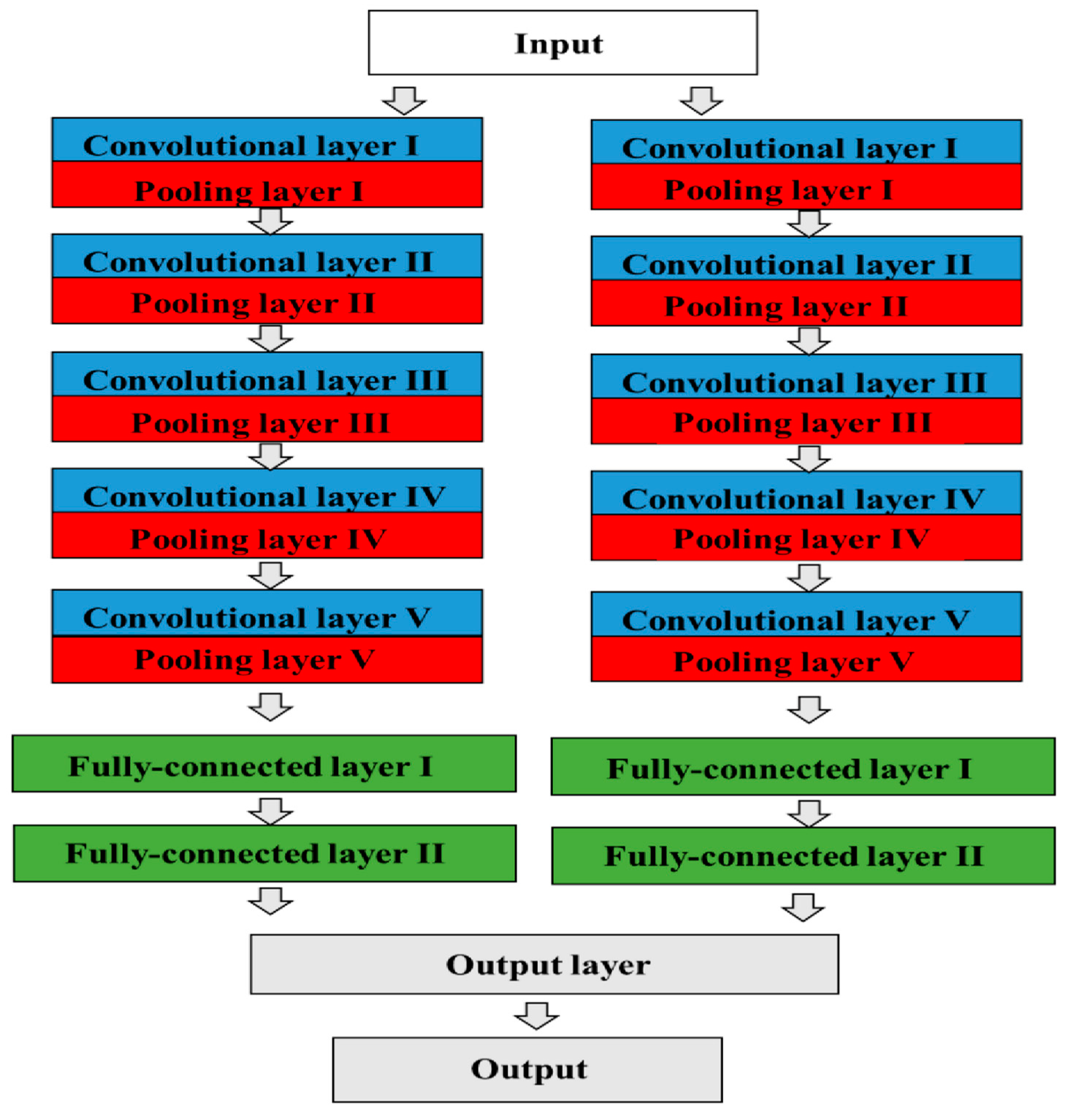
46]. CNN architecture, AlexNet, was designed by Alex Krizhevsky in collaboration with his Ph.D. supervisors, Ilya Sutskever and Geoffrey E. Hinton (
Figure 1) [
47,
48,
49]. This structure has five convolutional layers, some of which have max pooling layers. In addition, three fully connected layers with softmax functions are used for the output layer, so AlexNet contains eight layers in total. It is a variant of a CNN design published by Yann LeCun et al., and it applies backpropagation to Kunihiko Fukushima’s CNN architecture called Neo cognition [
50,
51,
52,
53,
54]. It adopts the rectified linear unit (ReLU) function, Dropout, and data expansion as features to improve accuracy [
55,
56]. The depth of the model is essential for high performance, and although it has a high computational cost, it was realized by using Graphic Processing Units (GPUs). A GPU Coder can be used to generate optimized code for prediction of various pretrained deep learning networks from a Deep Learning Toolbox.
Another type of CNN model is the visual-geometry group proposed in 2014 and announced by a research group at Oxford University. ImageNet is one such model, which has been implemented and pretrained and can be used easily. It is available in TensorFlow, PyTorch, etc., [
58,
59]. This model uses a CNN with 16 layers (VGG16) or 19 layers (VGG19) and, similar to AlexNet, it has a fully connected layer that greatly increases the number of parameters, resulting in a heavy network. However, it has good accuracy, is easy to use, and has a simple architecture. It uses many convolutions with a small 3 × 3 kernel size. After VGGNet, structures such as ResNet, with increasing numbers of channels, have been used in various models [
60,
61,
62,
63,
64,
65]. They repeat the flow of convolutions two or three times and then employ max pooling. Moreover, the number of channels is doubled by using a convolution after the pooling process and using ReLU as the activation function after each convolution. Each convolution has the following parameters: kernel size 3 × 3, stride 1, and padding size 1. This convolution is easy to use, in that the size of the feature map does not change, and it is widely used in other CNNs. Furthermore, connecting two 3 × 3 convolutions reduces the number of parameters, compared to one 5 × 5 convolution, and it has the same receptive field. This multiplexing of layers increases the number of times the activation function is applied, which increases its expressiveness. However, this structure has the problem that the number of parameters to be learned is relatively large, due to the large number of channels and the three fully connected layers at the end.
2.3. GoogLeNet
GoogLeNet is another pretrained CNN, which has 22 layers, and has won the 2014 Image Classification Challenge Contest (
Figure 2) [
66,
67,
68,
69]. The main feature of GoogLeNet is the Inception module, a small network that consists of multiple convolution layers, which convolve the original input image, and pooling layers, which reduce the original image while retaining important information. A large CNN can be constructed by stacking several Inception modules. The Inception module actively uses 1 × 1 convolutions—also called a bottleneck layer or pointwise convolution—which is a method for calculating by dividing the convolution into vertical and horizontal directions. The convolution in each channel direction has the same effect as dimensionality reduction, which reduces the number of calculations, and multiplex layers apply various transformations and concatenate them all together. This improves the drawback of CNNs, in which the image size decreases as the convolutional layers become deeper. Approximating the result with a small group of convolutional filters improves the trade-off between the expressiveness of the model and the number of parameters. In the convolution layer, this number is given by the number of input channels × number of output channels × kernel size, excluding the bias term. A normal convolution is dense because all parameters have some value, but Inception does independent convolutions of different sizes, which greatly reduces the number of non-zero parameters by applying multiple convolution layers in parallel and finally concatenating and processing the result of the computations.
In GoogLeNet learning, classification is performed even in sub-networks that branch from the middle of the network, and auxiliary loss is added to prevent the vanishing-gradient problem that occurs in machine learning when a neural network using a gradient-based learning method and error backpropagation becomes so small that learning becomes uncontrollable [
70,
71,
72]. When learning uses backpropagation, which computes the gradient of the loss function with respect to the weights of the network for a single input-output example, the weight of each node in the neural network is updated in proportion to the gradient obtained by partially differentiating the loss function calculated at each step with the weight of its node. The vanishing-gradient problem is caused by this gradient becoming so small that the neural network weights are less likely to be updated. In the worst case, weight updates may not occur at all. With classical activation functions such as a hyperbolic tangent function or a sigmoid function, the backpropagation method uses the chain rule, which works backward from the output layer of the neural network to calculate the partial derivative of the loss function concerning the weight of each node. As a result, by propagating the error directly to the middle layer of the network, vanishing gradients can be prevented and the network can be regularized. In addition, since the same effects as ensemble learning can be obtained, improvement in generalization performance can be expected. Moreover, even if the auxiliary loss is not introduced, learning may progress similarly by adding batch normalization. GoogLeNet also introduces Global Average Pooling (GAP) as another feature [
73]. A fully connected layer has conventionally been used as the last layer, but overfitting—a phenomenon that reduces versatility—has often been a problem. By adopting GAP instead of using fully connected layers, GoogLeNet reduces overfitting. A deep neural network is a mathematical model that mimics the human brain. It is a neural network with four or more layers that supports deep learning and deepens the layers. GoogLeNet can be thought of as a pretrained deep neural network since CNNs are a type of deep neural network. In addition, deep neural networks also include autoencoders that have the same input and output data. Recursive neural networks also exist. They are used for natural-language processing, e.g., for languages such as Japanese and English that humans normally use.
Furthermore, pre-learning is a technique in which each layer first learns and then is connected to other layers. This solves the vanishing-gradient problem that occurs when deep learning is performed because learning does not progress in the middle of a layer. A “pretrained deep neural network” is therefore a neural network with four or more layers designed to avoid the vanishing-gradient problem. GoogLeNet, a pretrained CNN, is designed to avoid the vanishing-gradient problem. It is a model that is mainly used in the field of image classification. The technology reads the elements of an image and determines the category to which it belongs. It achieves this using AI, which is a field in which CNNs such as GoogLeNet excel. Therefore, it can be used without training. To explain the mechanism of image classification simply, after inputting the original image, the image is converted into a form that can be categorized easily, and the elements are extracted and categorized in a format that is easy for the computer to understand. Based on the classification result, the image is classified into a category set by humans. Depending on the training dataset, the ImageNet dataset can classify images into 1000 types of object categories, such as keyboard, mouse, pencil, many animals, etc. Similarly, the Place365 dataset can classify images into 365 types of places, such as fields, parks, runways, lobbies, etc.
In addition, GoogLeNet is capable of transfer learning, which can further improve performance by generating new image-classification patterns and by creating a new model by slightly modifying what has been learned from a training model. This can shorten the learning time by eliminating the startup time required to collect data and learn it. In image classification using GoogLeNet, the sizes of images that can be processed in principle are 224 × 224 squares. Thus, it is necessary either to prepare a square image in advance and convert it into a square in the program, or program the system so that the image does not have to be a square. After reading the image and adjusting its size, GoogLeNet uses a function that performs the classification process, specifies the image above, and processes the classification. Finally, it displays the predicted category into which the read image has been classified.
2.4. Xception
Xception is an evolution of the GoogLeNet model; additionally, it is an improved model of the Inception method in GoogLeNet with a depth of 71 layers and ~5.5% error rate. A characteristic of the Xception architecture is the separable convolution layer, which can completely separate the information in the spatial direction and in the channel direction for convolution. Xception achieves high accuracy in large-scale image recognition with the same parameters through parameter reduction. Additionally, instead of ordinary convolution, Xception uses pointwise and depthwise convolutions, which have a skip connection, identity mapping, and no nonlinear function between depthwise and pointwise convolutions, instead of ordinary convolution. In contrast, Inception, the origin of Xception, contains a nonlinear function because the corresponding depthwise convolution does not convolve channel 1; hence, nonlinearity is important in such cases. As for computational complexity and the number of parameters in ordinary convolution layers, the input feature map size is F × F, the number of input channel size is N, the kernel size is K × K, and the number of output channels is M. Then, the computational complexity of this convolutional layer is F2NK2M because the cost of convolution per point in the input feature map is K2N, and by applying this to the F2 points in the input feature map, a 1-channel output feature map is generated, and there are M output feature maps. In M output feature maps, the amount of calculation is the same as above; however, there are M types of convolutions with K2N parameters, so it has K2NM parameters.
The key to Xception and MobileNets is to reduce the amount of computation and the number of parameters by devising the configuration of the convolutional layers. Particularly, while ordinary convolution convolves simultaneously in the spatial and channel direction of the feature map, both factorizes the channelwise (pointwise convolution) and the spacewise convolutions (depthwise convolution). The pointwise convolution is a 1 × 1 convolution used to skip connections such as ResNet. Although convolution in the spatial direction is not performed, convolution in the channel direction is performed. Pointwise convolution is the normal convolution, where K = 1; hence, the computational complexity is F2NM and the number of parameters is NM.
Alternatively, depthwise convolution performs spatial convolution for each channel of the feature map. Since convolution in the channel direction is not performed, the cost of one normal convolution is reduced from K2N to K2; therefore, the computational complexity of the convolution layer is F2NK2 and the number of parameters is K2N. Applying pointwise and depthwise convolutions as described above makes it possible to approximate an ordinary convolutional layer that simultaneously convolves in the spatial and the channel directions with fewer parameters and less computational complexity. Furthermore, computational complexity is reduced from F2NK2M to F2NM + F2NK2 and ratio to 1/K2 + 1/M. Usually, M >> K2 (e.g., K = 3 and M ≥ 32), then the computational complexity is reduced to ~1/9. Moreover, pointwise convolution is more of a bottleneck.
Xception model:
ReLU-depthwise-pointwise-BN-ReLU- depthwise- pointwise-BN- ReLU-depthwise- pointwise-BN (+identity mapping)
2.5. MobileNets
MobileNets are a class of efficient models designed for mobile and embedded vision applications, where computational, space, and power resources are typically limited. In the past, the focus of model development was to improve accuracy by making it deep and more complex. However, MobileNets was designed to maximize accuracy using the limited resources of on-device and embedded applications. MobileNet architecture is based on depthwise separable convolutions, which is a combination of depthwise and pointwise convolutions. The streamlined MobileNets architecture uses depthwise separable convolutions as the main building block of the network. MobileNets balance the trade-off between accuracy and speed by multiplying the number of channels in the feature map and the input image size by factors such as those with r < 1 while using the same network architecture. Therefore, the MobileNets realizes high-speed image recognition on Mobile while maintaining accuracy.
MobileNets model: depthwise-BN-ReLU- pointwise-BN- ReLU
3. Graphical Neural Networks (GNNs)
Graph theory is said to have started when Euler introduced it to problems such as the seven bridges of Königsberg [
74]. By definition, a graph is a data structure represented by objects (nodes) and relationships between them (edges). An adjacency matrix A that expresses whether there is a connection between two given nodes provides a representation for handling graphs mathematically [
75]. A degree matrix D represents the number of edges connected to each node. The Laplacian matrix L combines these two: L = D − A; it is normalized as follows:
where
N is the number of nodes.
The adjacency matrix
A = (
ai,j) of a graph
G = (
V,
E), where
V is the number of vertices (nodes), and
E is the number of edges, is a binary matrix that indicates whether two nodes are adjacent; i.e., whether there is an edge between them. It is defined as:
where
E is the number of edges.
The degree matrix
D = (
di,j) of a graph
G is a matrix in which the numbers of edges, bond degrees, containing nodes are arranged on the diagonal. It is defined as follows:
Conventional deep learning mainly deals with collections of individual data, vectors, data arranged in grids, images, and sequential data, text, or voice. Because of a lack of expressive power in dealing with various phenomena and data in the world, graph theory was incorporated into deep learning and developed. For example, there are many GNN models, which are neural networks designed for problems involving graphs, with graphs as the core for multivariate time series [
76,
77,
78,
79,
80]. In addition, graph-based machine learning is gaining increasing attention in many fields. For example, it is possible to understand an entire picture by processing local data separated by grids and overlaying several layers of CNNs. Graphs, on the other hand, do not care about Euclidean distance, and they can be used to combine data points related to an image and treat them as a data set.
Moreover, methods such as predicting ligand activity for compounds and target proteins are used in a variety of applications by extracting molecular features from the molecular structure using machine learning and using classification that evaluates the structural similarity of molecules. Among them, a molecular graph convolution neural network, which applies a deep learning model to chemical molecules, is used to more efficiently realize learning and analysis based on molecular structures.
Another approach is representation learning. Low-dimensional vectors can be used to represent nodes, edges, and subgraphs. While traditional methods of machine learning rely on manually setting feature values, graph-embedded methods can learn them instead. However, graphical methods also have their drawbacks; they are inefficient because parameters are not shared between nodes, and direct embedding cannot be generalized. Various GNN forms have therefore been proposed to address these deficiencies. However, graphs have the following difficulties, and deep learning, which has shown remarkable performance for data such as images and natural language, has had problems in applications to graphs. First, since a graph is not a tensor like an image, the definition of convolution is not trivial. Even searching on a graph is not easy; for example, no known algorithm can solve the problem of determining whether two graphs have the same shape in polynomial time (this is the “graph isomorphism problem”) [
81,
82,
83]. Furthermore, there are many different types of graphs, e.g., undirected/directed, weighted/unweighted, labeled/unlabeled, large/small, etc. The task to be solved for each is also different. In molecular-activity prediction, the goal is to regress some value from the entire graph. Therefore, different algorithms have to be designed for different tasks. In addition, memory and computational complexity become bottlenecks when dealing with large-scale graphs, so efficient algorithms must be devised.
Furthermore, information and constraints specific to the domain in which the graph appears may be intrinsically related to the task. For example, when treating a molecule as a graph, it is important to think about the algorithm that is to be used to determine the bond order and valence for each atom; for example, these quantities can only be suppressed to a maximum of about five for phosphorus (P). While such constraints can be used actively since the elements that determine the characteristics of the graph and the nodes to be handled differ from domain to domain, it is difficult to design a unified and general-purpose algorithm, and results tend to be scattered.
Over the past few years, many investigators have attempted to solve these problems by applying deep learning to graphs. The tasks that a GNN must perform include classification, regression, clustering, ranking, link prediction, and relationship prediction. Originally, graphs were often used to solve network-type optimization problems using nodes and edges. Combining a graph with a neural network has expanded these applications. By using neural networks, especially deep learning, it has become possible to extract feature values that could not be achieved with conventional network analysis.
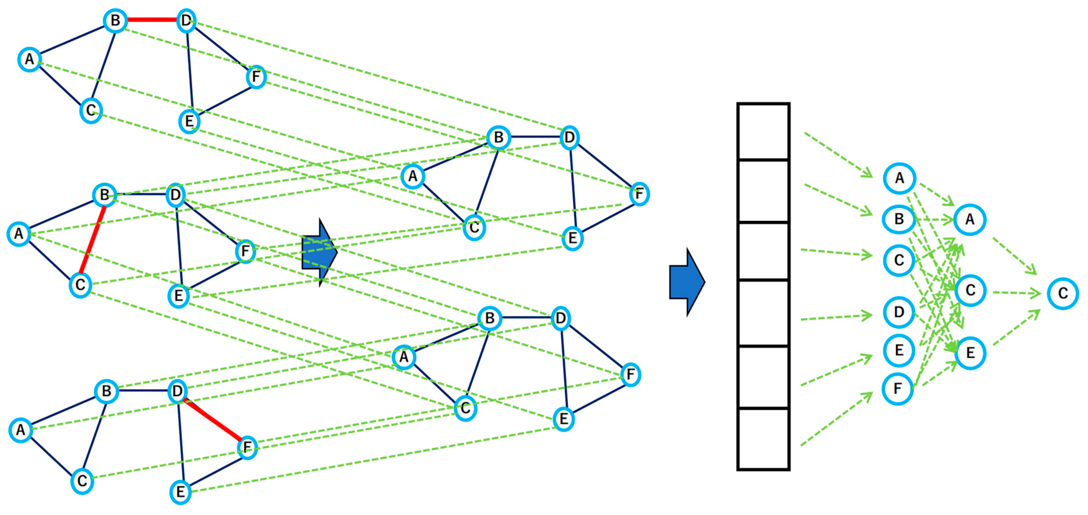
The concept of a GNN first appeared in 2005, and since then, there has been a boom in deep learning, and GNN research has become quite active. In particular, since 2016, major methods have emerged, such as that of a Gated GNN and Graph Convolution Network (GCN), which is an architecture that can learn embedded representations of nodes both with and without supervision based on the features of the nodes [
84,
85,
86,
87] (
Figure 3). When obtaining an embedding representation for node A on a graph with a two-layer GCN, the GCN computes the embedding representation of the node by repeated aggregation of neighboring nodes. The inner part of Equation (4) below represents the calculation of the first layer, in which node feature X is aggregated with the adjacency matrix A, a weight W is applied, and a nonlinear transformation is applied. The second layer receives representations of the nodes neighboring node A and computes an embedded representation of node A itself; this corresponds to the outer part of the formula below. The task on the graph is then solved using the final embedded representation of node A.
The disadvantage of a GCN is that—since the representation of a node is calculated by aggregating all adjacent nodes—if there is a node with a high degree, such as a node in a large-scale graph, the number of nodes to be calculated may increase accordingly.
A GNN repeats convolutions like a CNN. For example, a CNN convolves information from image data in eight directions: up, down, left, right, and obliquely. The difference is that a GNN convolves information either around a target node or for the entire graph. There are various types of GNN methods. When convolving information into nodes, the Aggregate and Combine processes are common, but the specific methods in the two are different. Aggregate performs the task of aggregating information from adjacent nodes, while Combine performs the task of updating node information from the information collected by Aggregate. When performing graph classification/regression tasks, the final feature value of the entire graph is generated by a method called Readout. In the most basic form of deep learning that deals with graphs, the latent vector hi for node i is obtained through the following steps. Using the learning function F(x), apply the following formula until the latent vector hi converges.
This captures the features around node
i. Then compute the output using the learned function
O(x):
Here,
F(x) and
O(x) can be modeled with an ordinary forward-propagating neural network [
85]. Weights are learned by iterative error backpropagation to minimize the error between
Yi and supervised labels (e.g., using the Almeida–Pineda algorithm). In addition, when obtaining the latent vector for the entire graph, it is possible to use the latent vector by considering something like a master node that is adjacent to all nodes. However, this method has several drawbacks and is not very practical. Step 1 does not end unless
F(x) is a contraction map. Since the recursive process in Step 1 is repeated, the amount of calculation is large. A gated-graph sequential neural network (GGS–NN) replaces the recursion process in Step 1 with a Gated Recurrent Unit (GRU), which is the gating mechanism in a recurrent neural network (RNN) and which has better performance on certain smaller datasets and removes the constraints of contraction mapping [
86,
87,
88,
89,
90,
91,
92]. The GRU concept can be expressed using the following formula:
That is, the hidden state ht is updated by the weighted sum of the following two elements. One is the hidden state ht−1 one step before. The other is a nonlinear transformation of the input xt and the hidden state r · ht−1 weighted by f. For example, if z = 1, the input is ignored, and the hidden state is preserved. Conversely, if z = 0, a new hidden state is calculated from a nonlinear transformation of the input and the hidden state. The quantity r affects the computation of new hidden states. If r = 0, the new hidden state is computed from the input only, while if r = 1, both the input and the hidden state are used. The values of z and r are also computed from xt and ht−1. Compared to a simple RNN, a GRU enables hidden-state retention by updating the gate z and thus providing long-term memory. In addition, a more compact hidden representation can be obtained by enabling the removal of hidden states using the initialization gate r.
GNN can handle atypical and complex data that cannot be handled by Multilayer perceptron, CNN, etc.; hence, most methods, such as deep learning, computer vision, natural language processing, etc., are developed based on a graph. Initially, graph theory was introduced as a one-stroke problem such as the Seven Bridges of Königsberg by Euler. Currently, it is widely applied to molecular structure analysis, etc. Graph is a data structure represented by objects (nodes) and relationships between them (edges). Conventional deep learning mainly deals with collections of individual data (vectors), data arranged in grids (images), and sequential data (text). Therefore, graph theory is adopted because it lacks expressive power when dealing with data. Specifically, understanding the whole picture is possible in CNN by processing local data separated using grids and overlaying several CNN layers. Conversely, the Euclidean distance is irrelevant in graphs, and data points related to “objects” can be combined and treated as a data set.
Another feature of GNN is representation learning. Low-dimensional vectors can represent nodes, edges, and subgraphs. In graph analysis, traditional machine learning methods rely on manually setting of the feature values, whereas graph-embedded methods can learn. However, it also has disadvantages: it is inefficient because parameters are not shared between nodes, and its direct embedding cannot generalize. Furthermore, an open problem with GNN is that they are vulnerable to adversarial attacks as a family of neural networks. In addition, GNN is entirely a black box, and only some explanations are available on the model based on examples. Furthermore, prelearning on graphs has just started, and their research has different problem settings and viewpoints; therefore, a wide range of research is still required in this field. Graphs are also becoming flexible. Thus, more complex graph structures and powerful models are required for real-world applications.
4. Current QSAR
The safety of chemical substances is generally evaluated through biological tests using animals, cells, microorganisms, etc. However, testing such a large number of chemicals is impractical due to labor, time, expense, and animal welfare considerations. Therefore, effective screening tools for rapid and accurate identification of hazardous chemicals without relying on biological testing are essential. Currently, several QSAR tools are used for hazard prediction, but the prediction results have not been practically used (
Table 1) [
92,
93,
94,
95]. In contrast, QSAR is a method for in silico prediction of chemical substances that are likely to cause adverse effects due to their chemical structures. Mutagenicity prediction with QSARs is one of the QSAR approaches used for assessing the effect of chemicals on the human health. This is a chemical structure–toxicity relationship study that predicts the toxicity of a substance based on the known activity of structurally similar substances without conducting biological toxicity tests. Because chemical toxicity is generally quantitatively correlated, toxicity by QSAR predicts an endpoint toxicity.
However, the mutagenicity test (genotoxicity test) is not a quantitative evaluation, but the results are binary regardless of whether they are mutagenic. Therefore, it is easy to verify the prediction model, that is, if the prediction is correct or incorrect. Currently, there are two main mutagenicity QSAR models: rule-based and statistical-based. The rule-based model defines characteristic substructures that bring about positive results from the known rule-based QSAR data, and qualitatively predicts test results based on ruled empirical rules. In contrast, statistics-based QSAR is an AI model that predicts test results using machine learning, such as multivariate analysis and pattern recognition, by converting the structure into geometric, electronic, and physicochemical descriptors, using those descriptors that are highly correlated with the positive test results after decomposing the structure of a chemical substance into fragments. As for these QSAR models, there are issues regarding prediction performance, selection of descriptors, or practical realization.
Furthermore, comparative molecular field analysis (CoMFA) attracts attention as a recent QSAR topic [
93]. Conventional QSAR can be analyzed in a relatively short time and is relatively easy-to-handle without requiring any special program software or computers. However, to handle only 2D structural formula information, it is difficult to explicitly handle 3D structural information of drugs, which is often important for the expression of drug activity. Therefore, in addition to the drug activity value, the 3D structure of the drug is input, as well as field data are calculated based on the 3D structure of the drug and the charge of each atom is used as a parameter. Finally, the partial least squares (PLS) method, which combines principal component analysis and multiple regression analysis, is used as a statistical analysis method. The field data are obtained by embedding a compound in a 3D lattice and calculating steric effects and electrostatic field representing the steric effect and the electronic effect, respectively, using probe atoms at each lattice point. Performing statistical analysis is possible using such grid point data that explicitly includes the 3D structure.
5. Deep Snap
Conventional machine learning approaches have the problem of reaching a plateau in predictive performance when building predictive models using large-scale input data as the number of times of learning increases. AI is also a promising tool for achieving advanced QSAR toxicity predictions [
98,
99,
100,
101]. Previously, molecular descriptors—which are indices that can be derived from the structure of the molecule, and which determine its properties, especially in the field of cheminformatics—have been used to transfer chemical-structure information to deep learning. However, since deep learning can directly use image information as input data, this conventional method indirectly uses the molecular structure and does not fully utilize the performance of deep learning. Therefore, one of us (Y.U.) developed a new structural-information input method called “Deep Snap” that is part of the image processing and allows learning of the characteristics of an entire molecule from image data [
102]. This method can automatically extract molecular features directly from the molecular structure without computing descriptors or the need for skilled techniques.
In the Deep Snap method, high-throughput conformer generation for large numbers of chemical compounds is first performed by a Molecular Operating Environment (MOE) application software program [
103] (
Table 2). Then, one three-dimensional (3D) structure per compound, defined with rotatable torsions, is optimized to generate a single low-energy conformation using the CORINA Classic software, and this is finally converted into the Simulation Description Format (SDF). In this format, 3D molecular structures are depicted as 3D ball-and-stick models, with different colors corresponding to different atoms. These are captured automatically as snapshots at user-defined angles on the x-, y-, and z-axes and saved as a PNG file with 256- × 256-pixel resolution (
Figure 4). All the PNG image files produced by Deep Snap are utilized as input datasets to the Nvidia Deep Learning GPU Training System (DIGITS) on a four-GPU system, Tesla-V100-PCIE, which is a pretrained open-source deep-learning model, Caffe with ILSVRC (ImageNet Large Scale Visual Recognition Challenge) 2012 dataset extracted from ImageNet using the CNN GoogLeNet, which is a 22-layer-deep CNN consisting of two convolutional layers, two pooling layers, and nine “Inception” modules. Each Inception module has six convolution layers and one pooling layer and utilizes four million parameters for image classification. It is implemented using open-source software on CentOS Linux (
Figure 5).
Numerous parameters must be adjusted to use the Deep Snap method. Previous investigations have studied the effects of the following parameters on the performance of the prediction models: (1) the number of molecules per SDF, (2) the zoom factor percentage, (3) the atom size for the van der Waals percentage, (4) the bond radius, (5) the minimum bond length, and (6) the bond tolerance [
57,
104,
105,
106]. The results suggest that optimal thresholds exist for attaining the best performance with these prediction models. In addition, using the Deep Snap approach with information about the chemical structure and activity from the Tox21 10K library, investigators have constructed 35 prediction models for nuclear-receptor agonists or antagonists [
107]. Three prediction models outperformed the best-performing models in the Tox21 Data Challenge 2014. However, the Deep Snap–Deep Learning method is a complex system that consists of four steps: the preparation of a 3D molecular structure from one-dimensional chemical information, the generation of a snapshot image of the 3D chemical structure, the construction of prediction models with deep learning, and statistical calculations.
To improve these complicated processes, a novel one-step system that executes Deep Snap sequentially using TensorFlow and Keras has been reported [
108]. The effects of angles on the generation of images have also been investigated using two Deep Snap systems: TensorFlow/Keras and DIGITS. Similar to the results obtained with DIGITS, the construction of a model showing high prediction performance has been observed with Deep Snap using TensorFlow/Keras. These results suggest that the 3D chemical-structure representation in the Deep Snap–Deep learning approach may be useful for molecular-image-based QSAR analyses, and improvements to the Deep Snap–Deep learning method may aid in achieving high-performing prediction models in various fields.
6. Explainability of Deep Learning
Unlike conventional machine learning models, neural networks, the underlying algorithms of deep learning technology, are characterized by reduced feature engineering costs with excellent discriminative and expressive power. However, the basis of the model’s judgment is difficult to interpret. This is called the “black box problem” and is one factor that makes applying AI technology in the society difficult. While this is applicable to machine learning in general, it is particularly challenging in neural networks. Generally, higher the complexity of a model, the more difficult it is to explain. For example, neural networks are more “complex models” than relatively simple decision trees. Since the black-box nature hinders the social implementation of AI, attention has been recently paid to the interpretability of AI and machine learning models. Therefore, AI that can explain the background of the output result and the basis of the judgment is generally called explainable AI, or XAI for short. Some XAI techniques can be applied to unstructured data, such as images, and structured data. Recently, the application scope of XAI has expanded, such as optimizing behavioral patterns for reinforcement learning.
The representative methods used to interpret models are divided into two approaches: (i) local surrogate and (ii) global surrogate. (i) Local explanations focus on specific input data samples and their prediction results, rather than the overall trend of the model, to interpret and visualize the basis for judgment. Specifically, predictive factors are estimated by approximating a complex model with a simple and highly readable linear model. For example, for tabular data, variables effective in predicting this time are calculated, and for image data, part of this image effective in predicting is calculated. Approximating the entire model can be complicated and difficult to understand, so it is important to focus on the prediction results of a single sample and provide an interpretation. Conversely, a global explanation analyzes the model as a whole and examines the contribution of each feature to interpret the prediction basis, such as Grad-CAM, which is a method for visualizing the prediction basis for the entire CNN model. The gradient information used by the CNN model for image classification gives the image recognition model a basis for judgment. The idea is to determine the pixels with high gradients, which significantly affect the predicted class output, and then assign weights to them. A heatmap then displays the range that CNN presumably analyzes for classification. In addition, local interpretable model-agnostic explanations (LIME), which is a representative technique for local explanations, approximates individual input data with a separate simple model. In contrast, the Grad-CAM method gives the deep learning model a basis for judgment.
Deep learning can achieve extremely high accuracy in specific fields, and its range of applications is expanding rapidly. However, such deep learning techniques also have weaknesses. Among them, the biggest problem is determining the basis for their judgment. Deep learning is good at learning the features in the data during the learning process. This eliminates the need for humans to extract features, but conversely, it is up to the network to decide which features to extract. As the name suggests, the extracted features have latent weights in the deep network, and it is challenging to extract the “something” that they learned in a form that humans can understand. In other words, “it should be learning something without knowing what it is learning”. This is the interpretability problem in deep learning. Sharing the process is important to be satisfied with the decisions made. Deep learning has made great strides in images, and these methods are an effective way to understand the decision-making process. First, the following two viewpoints exist for understanding the basis of deep learning decisions
Understanding the mechanism: Understand the process regarding the type of action performed by the model to reach the output (white box understanding).
Understanding behavior: Understand the output type depending on the input type (Black box understanding).
Since the “explanation” is given to humans, it must naturally be in an “expression” that humans can understand. However, it cannot explain even if it can “express”. Even if the expression is recognizable by humans, it may not have explanatory power. This difference between representation and description is defined as follows:
Representation: Human-understandable representation, converted explicitly into image (visualization) or text. However, the mere enumeration of numbers and words does not correspond to expressions.
Explanation: “Representing” the features (pixels in the input image, words in the input text, etc.) that contribute to the output of the network.
In other words, “explanation” is not simply “expression,” such as visualization or writing, but it becomes “explanation” only after “expressing” the feature value that contributes to the output of the network. Thus, there are two steps: (i) calculating the influence of each input on the output, and (ii) then expressing it in a human-understandable form.
Techniques for actually explaining the output of a network can be broadly divided into the following.
create an input that maximizes the output of the network
analyze the sensitivity of the input
reverse the path from the output to the input
estimate output trends from various inputs
infer judgment criteria from the amount of change
remediate learning results to be predictable
incorporate a point of view of the input into the model.
6.1. Activation Maximization
For a network dealing with classification problems, its output will have the classification probabilities for each category. Suppose we can find an input with a very high classification probability for a certain category, then the network regards it as a “representative example” of that category, and if it can be identified, it is useful for inferring the basis for judgment. When a network that has learned image features by unsupervised learning (autoencoder) performs classification, there arises a problem of finding
x* that maximizes the probability
p of being classified into class
c, which is the minimal input.
There is also a method to constrain it to be on the unit sphere by setting ||
x||
2 = 1. However, then the output will certainly be the maximum. Since there is a possibility of mysterious images that humans cannot understand, a state like overfitting, there is also a pattern that imposes a constraint closer to the actual input.
p(
x) means adding the probability that the data will appear. When the image features are visualized using equivalent constraints, and if the input data have high dimensions, it becomes very difficult to estimate this
p(
x) with high accuracy. Therefore, there is also a method of combining with generative models, such as variational autoEncoder (VAE) and generative adversarial networks (GAN), where
x* will be generated from a suitable vector
z through the generator.
The above equation shows the method of generating an image from z that is classified into class wc. In GAN, there is an equivalent constraint to this constraint, i.e., the constraint that the generated image is classified into the same class as the real class. However, what GAN aims for and what it aims for in understanding the basis for judgment are slightly different. In short, it is better to be somewhat abstract than something that looks real. Therefore, in the above equation, the λ||x||2 constraint is applied to suppress the width of the expression. However, deep dream uses this technique and optimizes the input image and random noise so that the output of the network is maximized.
6.2. Sensitivity Analysis
A feature is considered important if it considerably impacts the output by changing the output. In other words, the importance of an input can be understood by examining the amount of change that the network is sensitive to each input. This can be achieved by looking at the gradient since differentiation can reflect the amount of change in an output. Since neural networks primarily learn from gradients, this works well with existing optimization mechanisms. The sensitivity to the input x can be easily calculated as follows:
SmoothGrad is a device that makes it look more beautiful. Since the gradient is too sensitive to noise, it creates multiple samples with intentional noise and averages the results. From these results, it is possible to identify the part of the change that increases or decreases the error. For example, we know where to make the change to make it more like an object, but we do not know why it is judged as an object in the first place.
6.3. Deconvolution
The deconvolution method has been proposed, where the network is propagated to a certain layer and then back-propagated by setting zero to the part that need not be examined, and the input contribution to this part can be backcalculated. To remove negative values that attenuate the activation in this backpropagation, zero is set when the value becomes negative during propagation or backpropagation. This results in nonlinear processing that is equivalent to ReLU. We call this “guided backpropagation”. As a result, we have succeeded in visualizing the important points.
Since we want to know only the part that contributed to the classification of the class, a method of tracing the gradient backward from the desired label has also been proposed. This is a method for calculating the contribution of each feature map up to class classification and backpropagating with the weight. This allows you to obtain a heatmap-like output. However, since the contribution is calculated in map units, obtaining contributions in pixel units like the Guided backpropagation above is impossible.
In contrast, layer-wise relevance propagation (LRP) is a method that propagates the relationship between layers in reverse and reaches the input. The idea is that the sum of each input’s contribution to the output is equal across layers; only the distribution changes during propagation. PatternNet/patternAttribution has been proposed as an improved version of these methods. First, it is impossible to understand the basis for judgment simply by analyzing the “weights” in the network in this method. This is because the input x is first divided into s, which contributes to the final output y, and d; otherwise, s is noise and is expressed as x = s + d. Then, considering that the output of the simple network is wTx = y, weight w has the role of filtering d from x and extracting s, which contributes to y. The role of the weight w is to cancel the noise d; moreover, the vector direction of w depends on d, but it has no relationship with the desired s. Then, y = wTx = wT (s + d), and since d should be canceled by w, wTd = 0 and wTs = y. Furthermore, y and d should be completely uncorrelated, so cov[y,d] = 0, and cov [x,y] is equivalent to cov[s,y]. If the function to extract s from x is S(x), then cov[s,y] = cov[S(x),y]. Using this, S(x) can be obtained. First, in a linear transformation, s, which can only output linear y, should also be linear, so the correlation should be linear. Therefore, the following formula holds.
Substituting this into the cov relation above,
However, this is only a linear case and ReLU, which is often used for images, is a nonlinear function that does not propagate in the negative direction. In this case,
s and
d also need to be divided into
s+ and
d+ in the positive direction and
s− and
d− in the negative direction. Thus, the enhanced DeConvNet/GuidedBackpropagation or LRP, which replaces the backpropagated values with s+ and s−, are named as PatternNet or PatternAttribution, respectively. In addition, the extraction ability of
S(
x) can be measured using the following evaluation index ρ.
x − S(x) will have a very low correlation with wTx = y, resulting in a high value since only d is a remnant after s is completely passed through. Hence, estimating the basis for judgment with higher accuracy and measuring the estimation ability are possible.
6.4. LIME
The LIME method explores the behavior of the model not from a single input but from variously deformed inputs. First, an input is generated that looks like the original image is divided into several parts. Then, it is introduced to the trained model, and the decision result is obtained. This result gives us a pair of input and model decisions and is learned using a simple descriptive model prepared separately from the main model. This yields the most important features from a simple trained model. Because of the simplicity of the method, it can be applied to any model. Understanding black-box predictions using influence functions formulates the effect on the output of this input data fluctuation. It formulates the effect of each training data and the effect of changes to the training data; this makes it possible to identify samples that contribute to the decision of the model or decrease the decision accuracy, leading to changes that affect the decision of the model. In addition, a machine learning model of the LIME mechanism identifies what is important by masking the image, making it possible to visualize the important areas as masked areas.
6.5. Judgment Criteria Based on the Amount of Change
This is a method based on ensemble learning using decision trees. In each decision tree, the amount of change to bring one decision result to another decision result is calculated, and the smallest change is found among them. This method obtains the amount of change at the minimum cost.
6.6. Constraint
The concept is to control the overall tendency while taking advantage of the expressive power of the model, making it possible to reflect more detailed trends than accurately applying linear models. In some cases, it would be better to increase the amount of data in the first place, but there are often cases where it is not possible. Although there is a risk of not being able to respond to situations that should be handled by imposing restrictions, this method allows avoiding the risk of taking unpredictable behavior.
6.7. Attention
A method that introduces a mechanism that indicates the point of interest for the input data to the model is called “Attention”. The basic idea of Attention is to use the previously hidden layer and the past hidden layer when outputting. At that time, the weight is distributed based on the important points. For example, when the hidden layer at time t is ht and the past hidden layer is hs, the attention (weight) for them can be defined as follows.
Many score variations exist, such as simply taking the inner product or preparing weights for attention.
Then, multiply this attention (weight) to create a vector (context) c for output at time
t, i.e., calculate the weighted average.
7. Discussion
QSAR and read-across predictions based on grouping approaches have been widely used in the evaluation of pharmaceuticals and general chemical substances because they provide information, such as target endpoints, without conducting tests. Additionally, even in the Integrated Assessment and Testing Strategy, a new evaluation system that leads to efficient testing and evaluation without conventional testing systems based mainly on animal tests, predictions by QSAR/read-cross, etc. play an important role. In this way, methods for predicting the activity of substances without conducting tests include the QSAR model and the grouping approach, which is a general term for the analog/category approach. Furthermore, the prediction of various properties of compounds is also carried out in fields such as pharmacological activity and physical properties; however, the application method is considerably different from that used for toxicity and its side effects. Once the mechanism of pharmacological activity is clarified, predicting the activity of a compound is possible based on the mechanism. QSAR is developed on the basis of drug thermodynamics such as the movement of drugs from extracellular to intracellular and reactivity at various receptor sites. In the docking approach, once the receptor enzyme and the docking site are clarified, designing suitable compounds is possible by predicting the pharmacological activity. In the field of toxicity or side effect prediction research, prediction was initially conducted by chemical multivariate analysis or pattern recognition, and chemometrics. Since then, rule-based AI has been implemented as AI-related technologies have improved. Thus, there are currently only two types of in silico methods applied to predict toxicity and side effects: (1) approaches based on chemical multivariate analysis or pattern recognition, chemometrics, etc. and (2) approaches based on rule-based AI. Compared with pharmacological activity and physical properties of drugs, various factors are involved in its toxicity and side effects, making prediction difficult and limiting application methods. Therefore, the prediction of toxicity and side effects of drugs is challenging, and the application of in silico computer methods for their prediction is severely limited. Furthermore, when considering individual methods for compound structure variability, the QSAR response level is low as it is theoretically developed based on drug thermodynamics. Therefore, the QSAR formula can only be applied if the compound structure has the same basic skeleton and the positions of the substituents must also be fixed. In other words, the prediction reliability of the QSAR formula is extremely high as long as the restrictions for this compound’s structural formula are satisfied. However, the application of the QSAR formula to compounds that do not meet this structural formula restriction ignores the basic principle; hence, even if the prediction results are obtained in such cases, they are completely unreliable. Basically, the prediction by the QSAR formula can be performed only when structural formula restrictions are satisfied, and there is no point in applying it to compounds that exceed the structural restrictions even a little. Furthermore, toxicity and side effect prediction of drugs basically needs to correspond to all compounds. In this respect, QSAR has very little tolerance for compound structural variability; hence, it is a method that is difficult to apply for toxicity and side effect prediction.
Conversely, chemical multivariate analysis or pattern recognition and AI methods can handle all compounds based on the application principle; in this respect, the ability to respond to compound structural variability is extremely high. Therefore, it is highly possible to deal with compound structure variability, which is the biggest problem in predicting toxicity and side effects. This point is a major reason why these two methods have been applied not only in the past but are also used at present to predict toxicity and side effects.
Additionally, in the case of ADME/T prediction, the expression mechanism is complicated/difficult to identify, especially for toxicity and side effect prediction; furthermore, it is not possible to identify the information on enzymes and receptor sites required for structure-based drug-design (SBDD) and 3D-QSAR implementation. Therefore, SBDD and 3D-QSAR procedures cannot predict ADME/T. In future, it may be possible to apply it to ADME/T if research based on the adverse outcome pathway (AOP) concept is actively pursued in the field of toxicity, and the toxicity manifestation mechanism becomes clear. Since QSAR is based on drug thermokinetics, it also partially involves pharmacokinetics and pharmacodynamics of ADME.
To date, the QSAR system using deep learning has been applied in various fields, but the QSAR system using 3D-chemical structure information has not yet been applied except for Deep Snap. The prediction model constructed using Deep Snap showed a predictive performance better than that of conventional machine learning methods such as random forest and XGBoost. However, further improvement is needed to reduce the computational cost, simplify the method, and achieve high throughput. In general, when learned with deep learning, a reasonable performance can be demonstrated if there are about 5000 data per class. However, if human-level accuracy is desired, a large-scale labeled data set of about 10,000,000 items is essential.
In addition, despite the high predictive ability of the Deep Snap prediction model, the explainability by which features extracted from CNN in the Deep Snap–Deep Learning remains unclear. In other words, it is important to specify the part to be extracted as a feature value by CNN and to interpret the predictions. Evaluations involving other biomolecules in toxicology and biological systems are similarly applicable by delineating 3D-chemical structures using Deep Snap.
8. Conclusions
Recently, from the viewpoint of animal welfare 3R (replacement: use of alternative methods, reduction: reduction of the number of animals used, and refinement: reduction of suffering), the adoption of alternative methods for animal testing is progressing even for chemical substances. Among these, in silico alternatives for animal experiments have been developed for a long time, and QSAR is one of the most utilized methods. However, QSAR has problems, such as its prediction performance, generalizability, and ability to process significant amounts of data. Alternatively, prediction models using deep learning have recently been shown to have high prediction performance and high data processing capacity and are hence receiving attention. In this review, we demonstrated that a novel QSAR system using deep learning based on molecular images can construct models with a high prediction performance. Furthermore, by using 3D structural information, this system may be able to utilize more structural information than predictive models using 2D graphs. Therefore, this new system will be a powerful tool for predictive modeling in various fields.


