
Coil High Voltage Spark Plug Boots Insulators Material Selection Using MCDM, Simulation, and Experimental Validation


Abstract
:1. Introduction
2. Materials and Methods
2.1. Piece Performance
2.2. Materials
- Possessing the dielectric, thermal, chemical, mechanical, and other properties required to carry out the specified function.
- Being widely accessible;
- Having a reasonable price.
2.3. Multicriteria Selection Methods and Weighting Method
2.3.1. Statistical Variation Method
2.3.2. VIKOR Method
2.3.3. PUGH Method
- Assign point value to each criterion and build the decision matrix. For this, the matrix of the Entropy method is used.
- Give positive (+) or negative (−) values to the characteristics, according to what is sought and build the prioritization matrix. In this matrix, the criteria of the options are compared with the original criteria.
- Numerical values are assigned to this comparison, where better than the original = 1, same as original = 0, and worse than the original = −1
- The third step in obtaining the weighting matrix is to apply,
- Raking. It is the step in which the alternative with the best results must be selected and given a place on the scale, the first position being occupied by the one with the highest value.
2.3.4. TOPSIS Method
2.3.5. PROMETHEE II Method
2.3.6. DOMINIC Method
2.3.7. COPRAS Method
2.3.8. Spearman Correlation Coefficient
2.4. Simulation
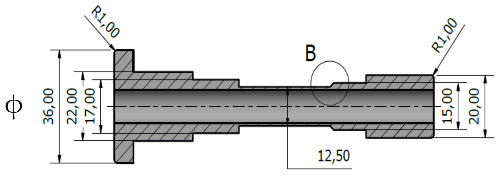
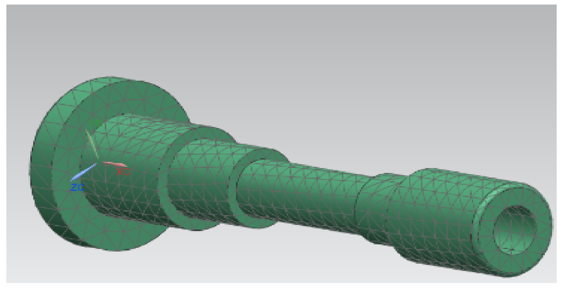
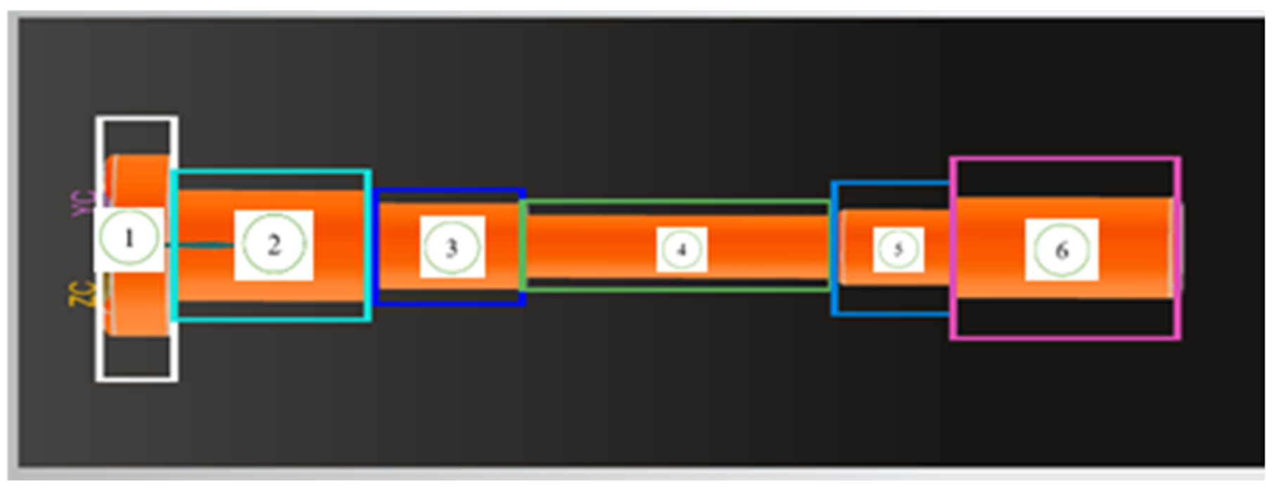
2.4.1. CAD Model
2.4.2. Thermal Simulation
2.4.3. Conditions for the Simulation
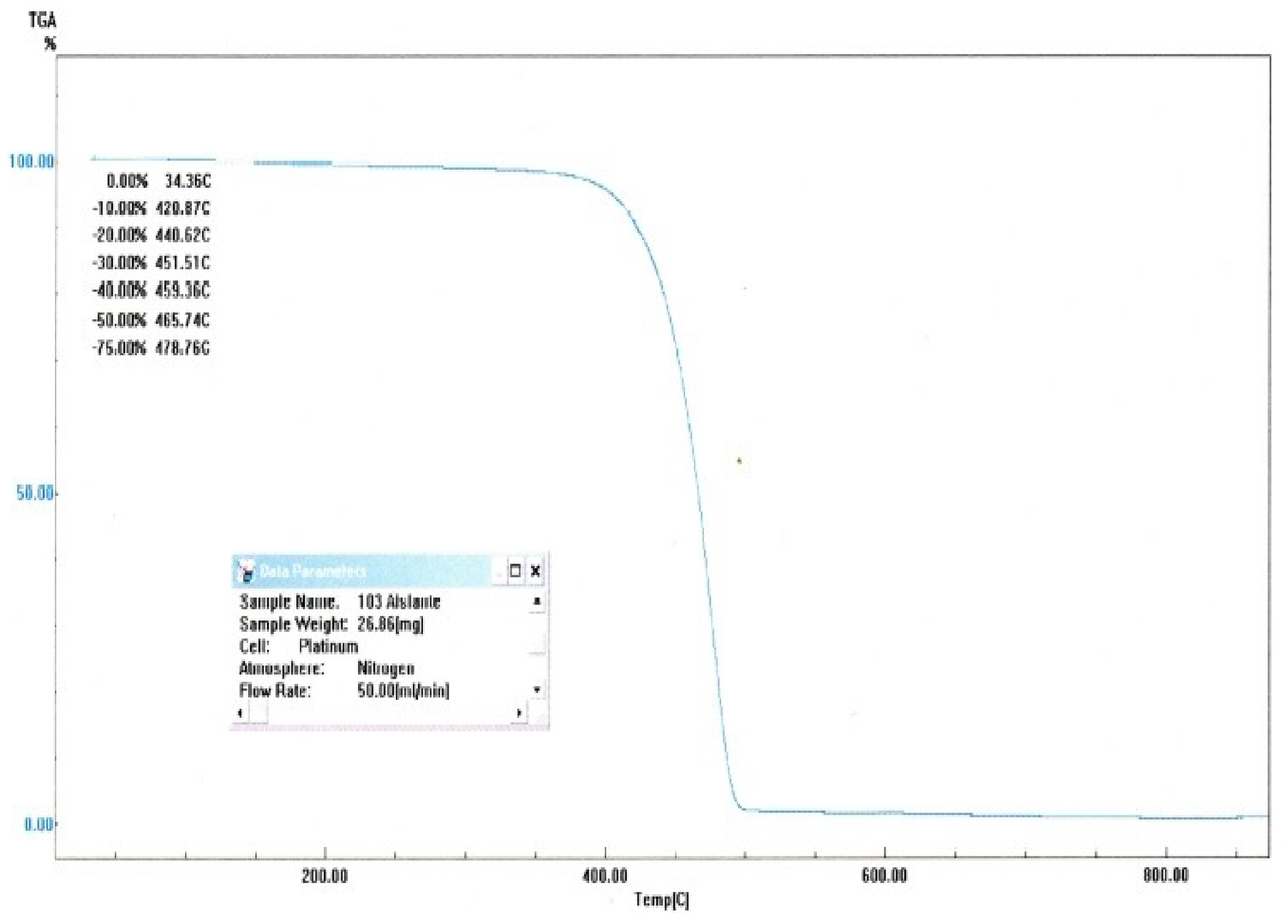
2.5. Thermogravimetry Test
3. Results
3.1. Results of the MCDM
3.1.1. Results of the Statistical Variation Method
3.1.2. Results of the VIKOR Method
3.1.3. Results of the PUGH Method
3.1.4. Results of TOPSIS Method
3.1.5. Results of the PROMETHEE II Method
3.1.6. Results of the DOMINIC Method
3.1.7. Results of the COPRAS Method
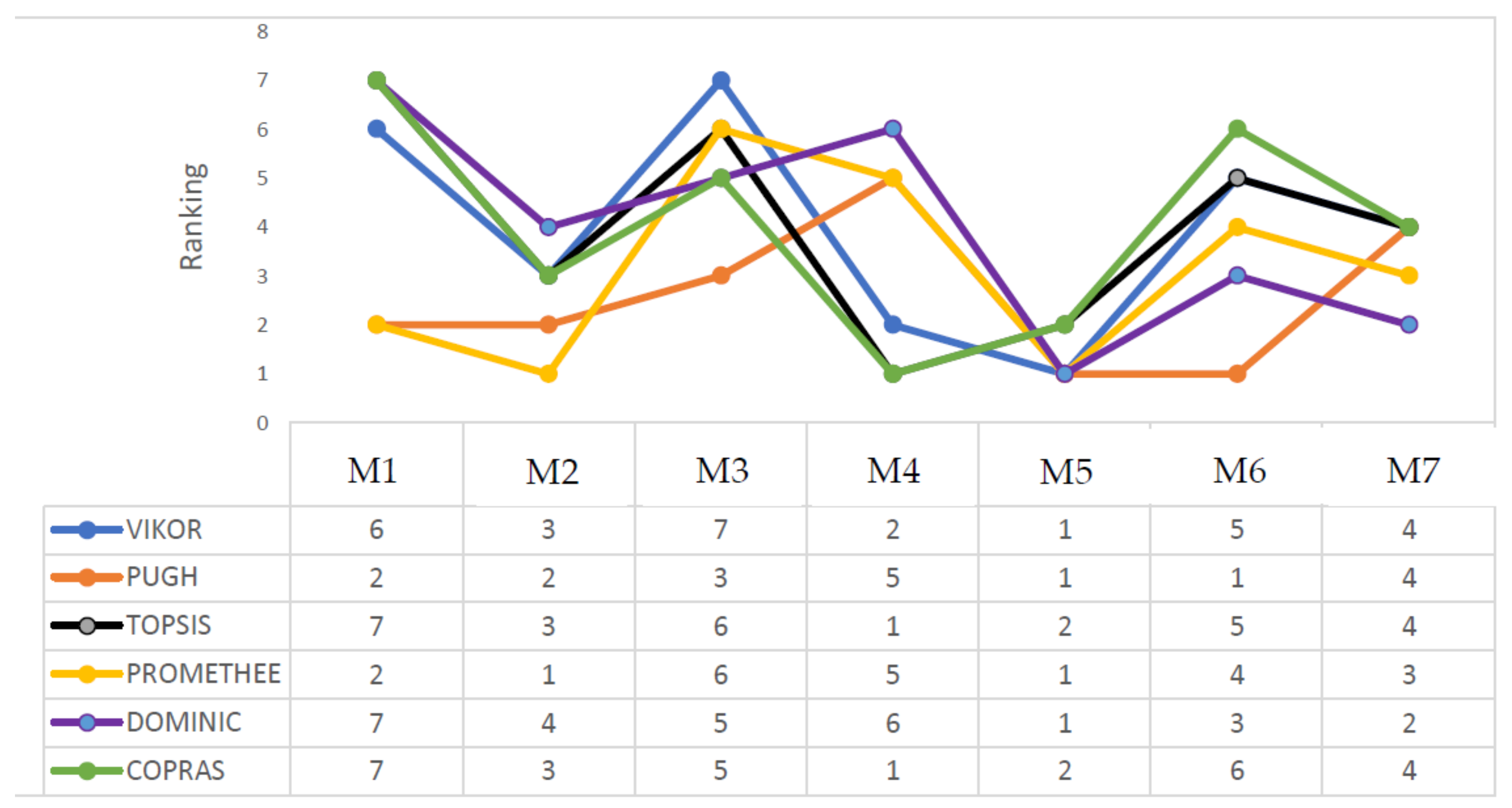
3.1.8. Evaluation of the Results for the MCDM Methods
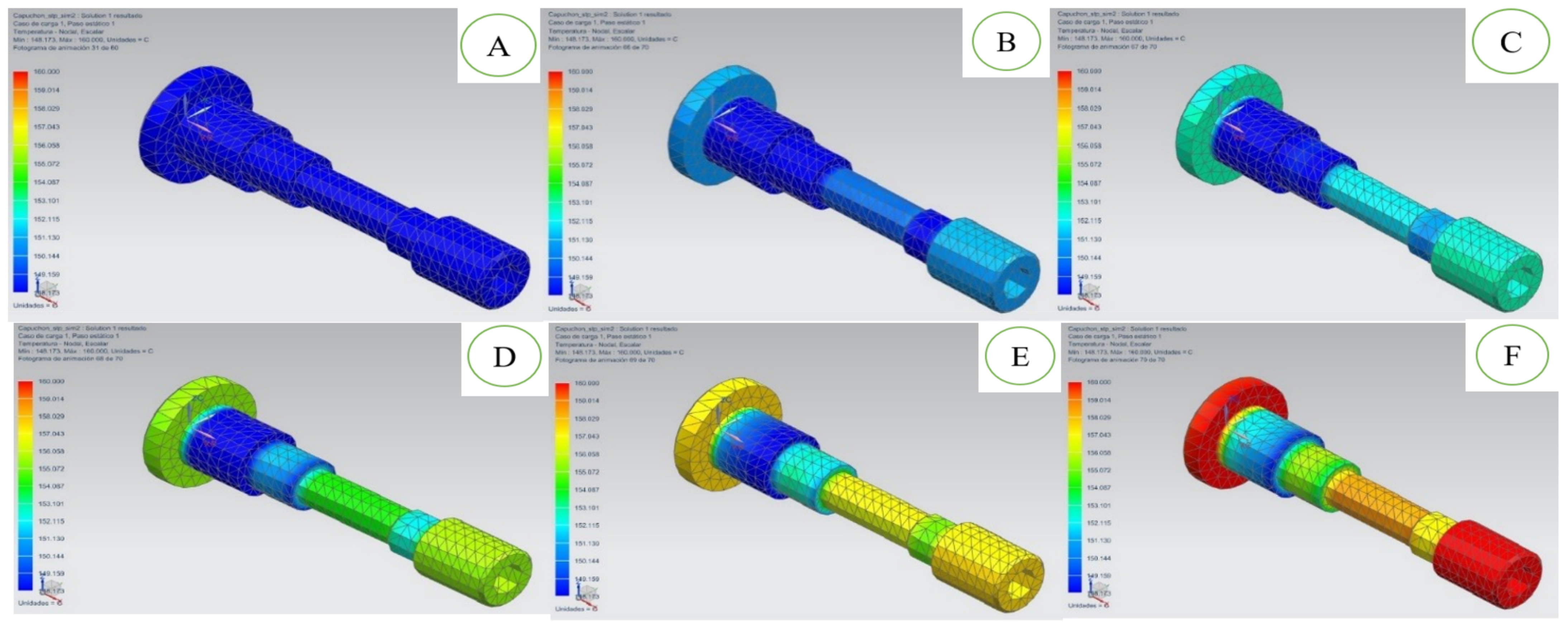
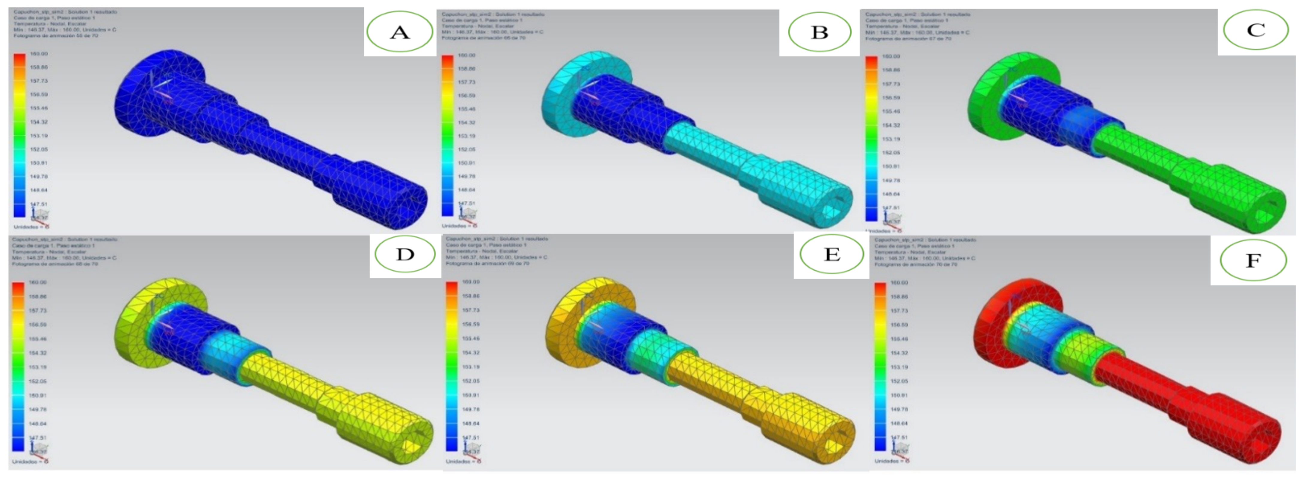
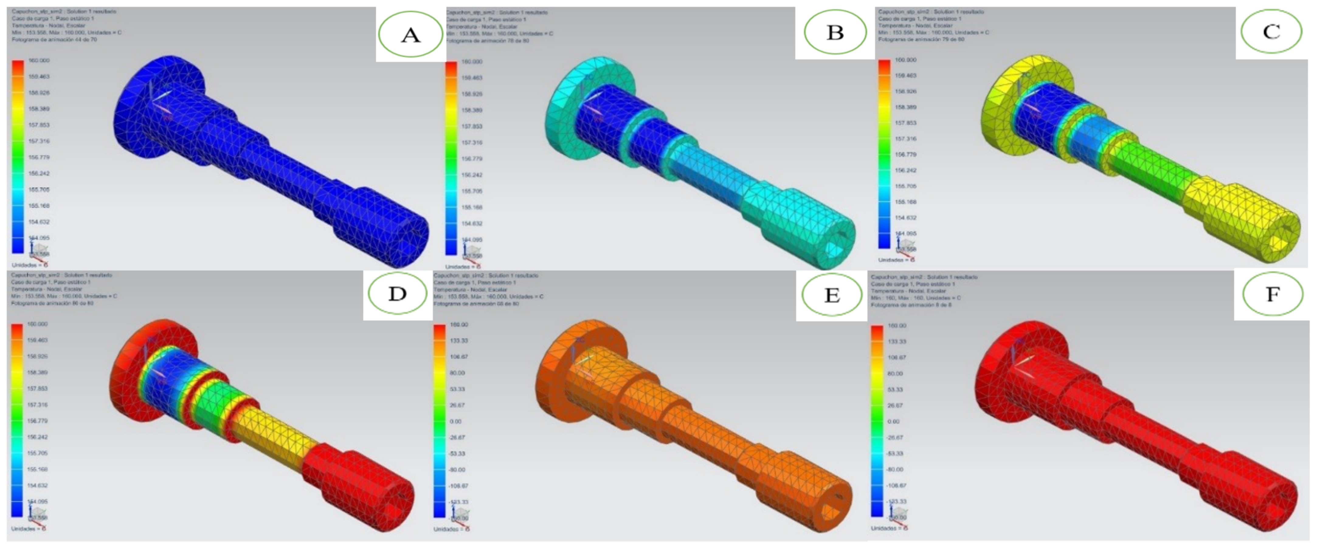
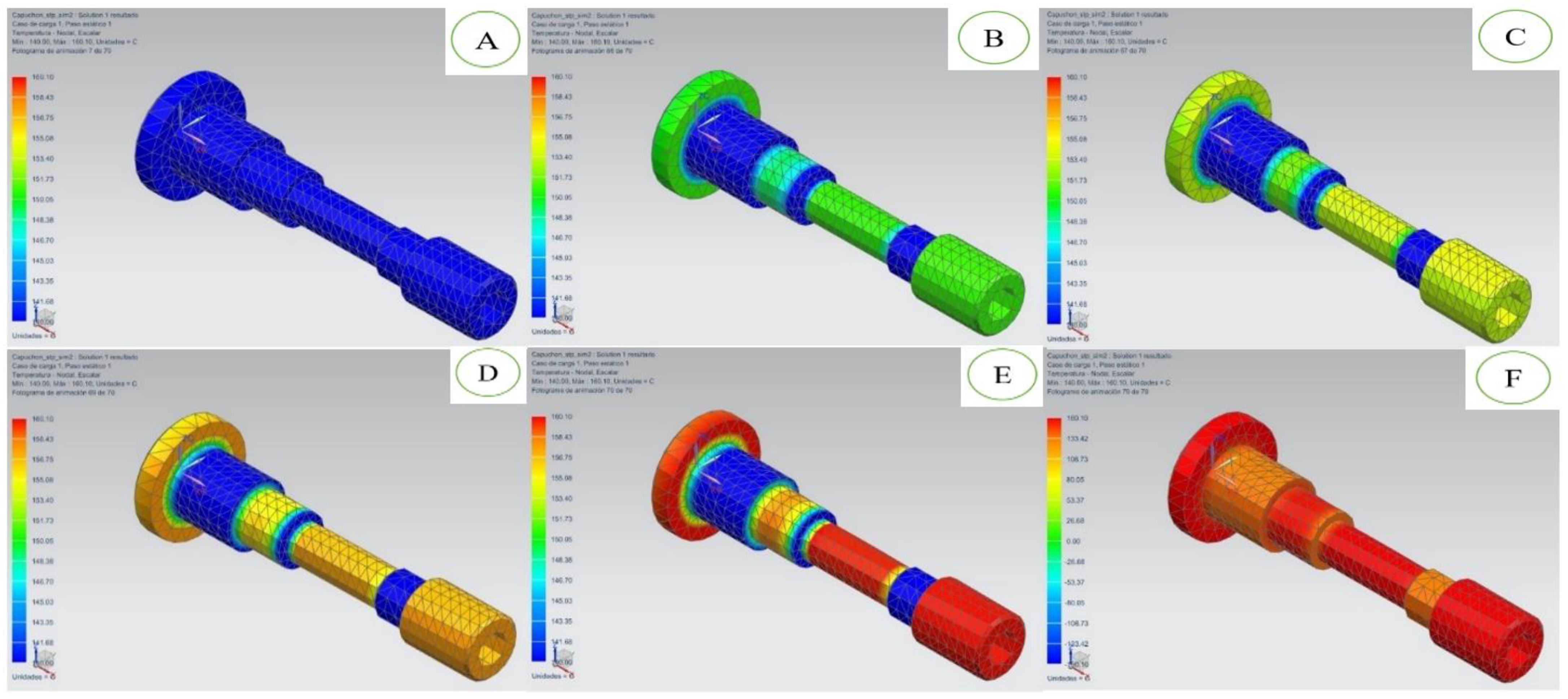
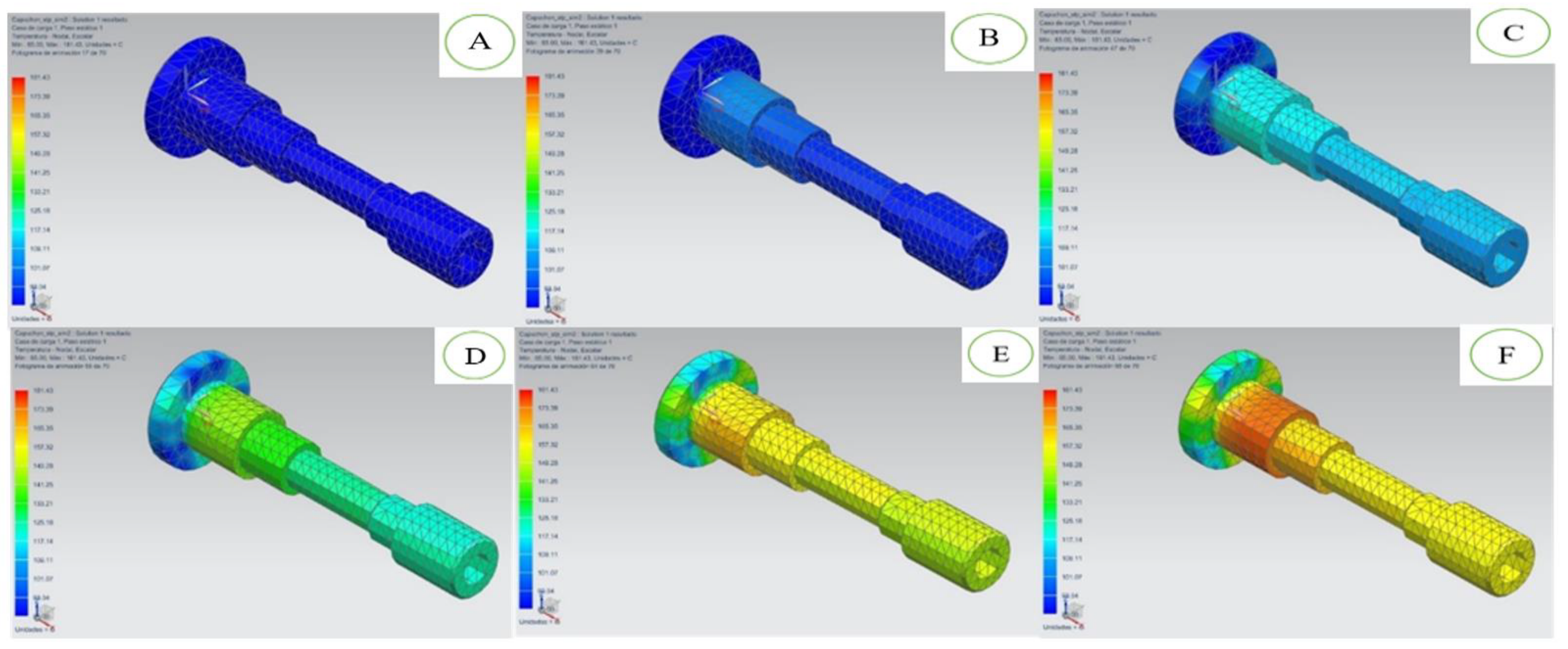
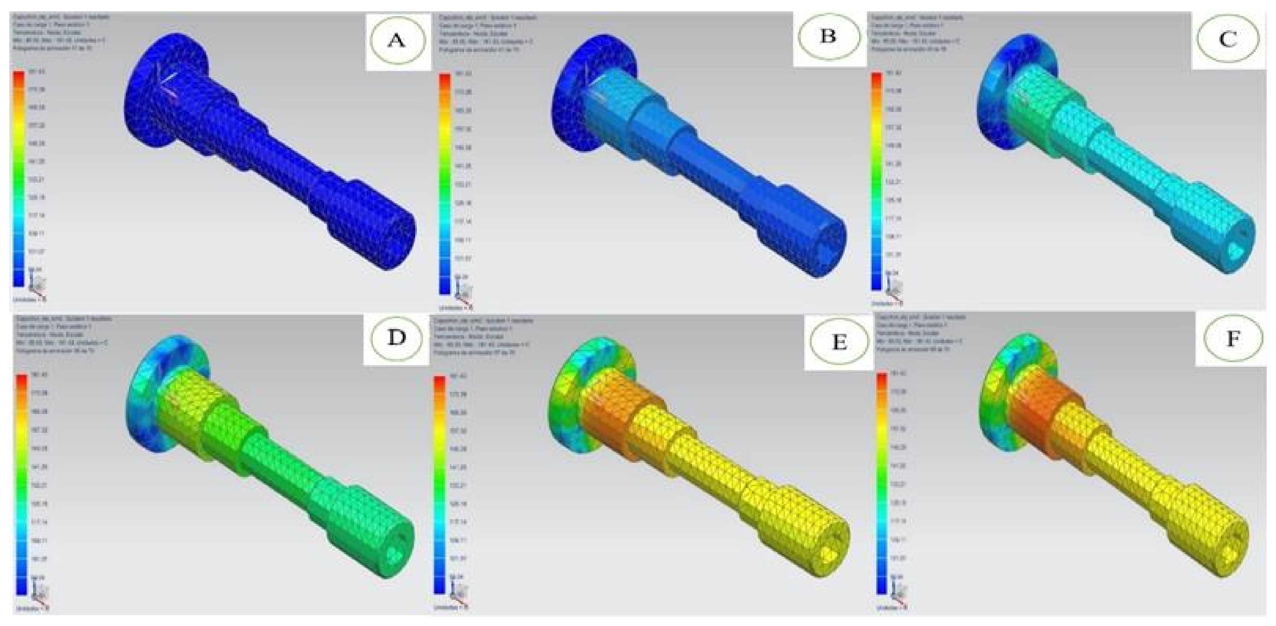
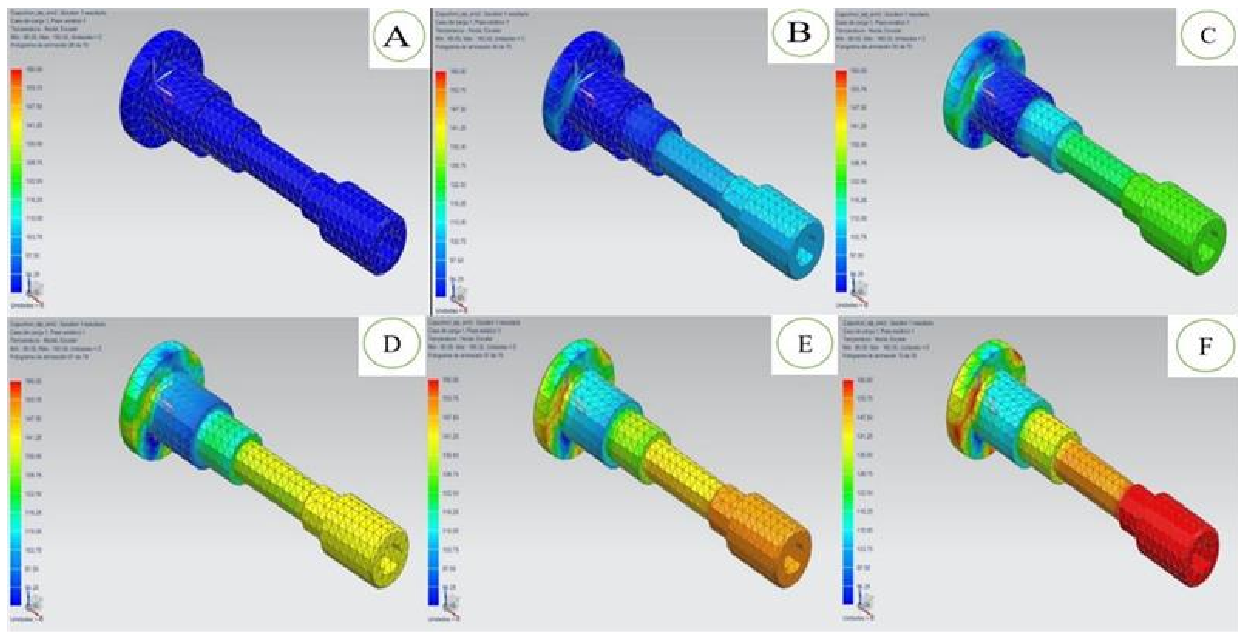
3.2. Results of Simulation
3.2.1. Results of Simulation with Polyethylene LDPE
3.2.2. Results of the Simulation with Polythene HDPE
3.2.3. Results of the Simulation with Polystyrene
3.2.4. Results of Simulation with PVC
3.2.5. Results of the Simulation with Nylon
3.2.6. Results of the Simulation with Teflon
3.2.7. Results of the Simulation with Polypropylene
3.2.8. Results of the TGA
4. Conclusions
Author Contributions
Funding
Data Availability Statement
Acknowledgments
Conflicts of Interest
References
- Ashby, M.F.; Cebon, D. Materials selection in mechanical design. J. Phys. IV 1993, 3, C7-1. [Google Scholar] [CrossRef]
- Villacreses, G.; Gaona, G.; Martínez-Gómez, J.; Jijón, D.J. Wind farms suitability location using geographical information system (GIS), based on multi-criteria decision making (MCDM) methods: The case of continental Ecuador. Renew. Energy 2017, 109, 275–286. [Google Scholar] [CrossRef]
- Caliskan, H.; Kursuncu, B.; Kurbanglu, C.; Güven, S. Material selection for the tool holder working under hard milling conditions using different multi criteria decision making methods. Mater. Des. 2013, 45, 473–479. [Google Scholar] [CrossRef]
- Aly, M.F.; Hamza, K.T.; Farag, M.M. A materials selection procedure for sandwiched beams via parametric optimization with applications in automotive industry. Mater. Des. 2015, 56, 219–226. [Google Scholar] [CrossRef]
- Jahan, A.; Ismail, M.Y.; Sapuan, S.M.; Mustapha, F. Material screening and choosing methods—A review. Mater. Des. 2010, 31, 696–705. [Google Scholar] [CrossRef]
- Bitarafan, M.; Zolfani, S.H.; Arefi, S.L.; Zavadskas, E.K. Evaluating the construction methods of cold-formed steel structures in reconstructing the areas damaged in natural crises, using the methods AHP and COPRAS-G. Arch. Civ. Mech. Eng. 2012, 12, 360–367. [Google Scholar] [CrossRef]
- Findik, F.; Turan, K. Materials selection for lighter wagon design with a weighted property index method. Mater. Des. 2012, 37, 470–477. [Google Scholar] [CrossRef]
- Rangaiah, G.P.; Feng, Z.; Hoadley, A.F. Multi-Objective Optimization Applications in Chemical Process Engineering: Tutorial and Review. Processes 2020, 8, 508. [Google Scholar] [CrossRef]
- Godoy-Vaca, L.; Almaguer, M.; Martínez-Gómez, J.; Lobato, A.; Palme, M. Analysis of Solar Chimneys in Different Climate Zones-Case of Social Housing in Ecuador. In IOP Conference Series: Materials Science and Engineering; No. 7, 072045; IOP Publishing: Bristol, UK, 2019; Volume 245. [Google Scholar]
- Kastillo, J.P.; Martínez-Gómez, J.; Villacis, S.P.; Riofrio, A.J. Thermal Natural Convection Analysis of Olive Oil in Different Cookware Materials for Induction Stoves. Int. J. Food Eng. 2017, 13. [Google Scholar] [CrossRef]
- Gomes, L.C.; Miranda, J.; Mergulhão, F.J. Operation of Biofilm Reactors for the Food Industry Using CFD. In Computational Fluid Dynamics in Food Processing; CRC Press: Boca Raton, FL, USA, 2018; pp. 561–590. [Google Scholar]
- Kastillo, J.P.; Martínez, J.; Riofrio, A.J.; Villacis, S.P.; Orozco, M. A Computational fluid dynamic analysis of olive oil in different induction pots. In Proceedings of the 1st Pan-American Congress on Computational Mechanics–PANACM, Buenos-Aires, Argentina, 27–29 April 2015; pp. 729–741. [Google Scholar]
- Beltrán, R.D.; Martínez-Gómez, J. Analysis of phase change materials (PCM) for building wallboards based on the effect of environment. J. Build. Eng. 2019, 24, 100726. [Google Scholar] [CrossRef]
- Anderson, A.; Coughlan, B. Liquid film flows over solid surfaces. In Proceedings of the 6th MIRA International Vehicle Aerodynamics Conference, Gaydon, UK, 25–26 October 2006; pp. 368–379. [Google Scholar]
- Bouchet, J.P.; Delpech, P.; Palier, P. Wind tunnel simulation of road vehicle in driving rain of variable intensity. In Proceedings of the MIRA Aerodynamics Conference, Warwick, UK, 13 October 2004. [Google Scholar]
- Gaylard, A.P.; Duncan, B. Simulation of rear glass and body side vehicle soiling by road sprays. SAE Int. J. Passeng. Cars-Mech. Syst. 2011, 4, 184–196. [Google Scholar] [CrossRef]
- Gaylard, A.P.; Kirwan, K.; Lockerby, D.A. Surface contamination of cars: A review. Proc. Inst. Mech. Eng. Part D J. Automob. Eng. 2017, 231, 1160–1176. [Google Scholar] [CrossRef]
- Wu, Y.S.; Cui, W.C. Advances in the three-dimensional hydroelasticity of ships. Proc. Inst. Mech. Eng. Part M J. Eng. Marit. Environ. 2009, 223, 331–348. [Google Scholar] [CrossRef]
- Skinner, A.A.; Lovers, H.O. Ignition Coil. U.S. Patent 7,268,655, 25 August 2015. [Google Scholar]
- Rao, R.V. A decision making methodology for material selection using an improved compromise ranking method. Mater. Des. 2008, 29, 1949–1954. [Google Scholar] [CrossRef]
- Aldás, P.S.D.; Constante, J.; Tapia, G.C.; Martínez-Gomez, J. Monohull ship hydrodynamic simulation using CFD. Int. J. Math. Oper. Res. 2019, 15, 417–433. [Google Scholar] [CrossRef]
- Turner, A. Foamed polystyrene in the marine environment: Sources, additives, transport, behavior, and impacts. Environ. Sci. Technol. 2020, 54, 10411–10420. [Google Scholar] [CrossRef]
- Xu, S.; Camp, C.H., Jr.; Lee, Y.J. Coherent anti-Stokes Raman scattering microscopy for polymers. J. Polym. Sci. 2022, 60, 1244–1265. [Google Scholar] [CrossRef]
- Acurio, K.; Chico-Proano, A.; Martínez-Gómez, J.; Ávila, C.F.; Ávila, Á.; Orozco, M. Thermal performance enhancement of organic phase change materials using spent diatomite from the palm oil bleaching process as support. Constr. Build. Mater. 2018, 192, 633–642. [Google Scholar] [CrossRef]
- Rahim, A.A.; Musa, S.N.; Ramesh, S.; Lim, M.K. A systematic review on material selection methods. Proc. Inst. Mech. Eng. Part L J. Mater. Des. Appl. 2020, 234, 1032–1059. [Google Scholar] [CrossRef]
- Kabak, Ö.; Ervural, B. Multiple attribute group decision making: A generic conceptual framework and a classification scheme. Knowl.-Based Syst. 2017, 123, 13–30. [Google Scholar] [CrossRef]
- Chingo, C.; Martínez-Gomez, J. Material selection using multi-criteria decision making methods for geomembranes. Int. J. Math. Oper. Res. 2020, 16, 24–52. [Google Scholar] [CrossRef]
- Wang, C.N.; Yang, F.C.; Vo, N.T.; Nguyen, V.T.T. Wireless communications for data security: Efficiency assessment of cybersecurity industry—A promising application for UAVs. Drones 2022, 6, 363. [Google Scholar] [CrossRef]
- Dang, T.T.; Nguyen, N.A.T.; Nguyen, V.T.T.; Dang, L.T.H. A two-stage multi-criteria supplier selection model for sustainable automotive supply chain under uncertainty. Axioms 2022, 11, 228. [Google Scholar] [CrossRef]
- Liu, H.C.; Liu, L.; Wu, J. Material selection using an interval 2-tuple linguistic VIKOR method considering subjetive and objetive weights. Mater. Des. 2015, 52, 158–167. [Google Scholar] [CrossRef]
- Huynh, T.T.; Nguyen, T.V.; Nguyen, Q.M.; Nguyen, T.K. Minimizing warpage for macro-size fused deposition modeling parts. Comput. Mater. Contin. 2021, 68, 2913–2923. [Google Scholar]
- Mousavi-Nasab, S.H.; Sotoudeh-Anvari, A. A new multi-criteria decision making approach for sustainable material selection problem: A critical study on rank reversal problem. J. Clean. Prod. 2018, 182, 466–484. [Google Scholar] [CrossRef]
- Wang, X.; Zhang, R.; Zhang, K.; Shao, L.; Xu, T.; Shi, X.; Li, D.; Zhang, J.; Xia, Y. Development of a Multi-Criteria Decision-Making Approach for Evaluating the Comprehensive Application of Herbaceous Peony at Low Latitudes. Int. J. Mol. Sci. 2022, 23, 14342. [Google Scholar] [CrossRef]
- Villacreses, G.; Martinez-Gomez, J.; Jijon, D.; Cordovez, M. Geolocation of photovoltaic farms using Geographic Information Systems (GIS) with Multiple-criteria decision-making (MCDM) methods: Case of the Ecuadorian energy regulation. Energy Rep. 2022, 8, 3526–3548. [Google Scholar] [CrossRef]
- Nenzhelele, T.; Trimble, J.A.; Swanepoel, J.A.; Kanakana-Katumba, M.G. MCDM Model for Evaluating and Selecting the Optimal Facility Layout Design: A Case Study on Railcar Manufacturing. Processes 2023, 11, 869. [Google Scholar] [CrossRef]
- Nicolalde, J.F.; Cabrera, M.; Martínez-Gómez, J.; Salazar, R.B.; Reyes, E. Selection of a phase change material for energy storage by multi-criteria decision method regarding the thermal comfort in a vehicle. J. Energy Storage 2022, 51, 104437. [Google Scholar] [CrossRef]
- Nicolalde, J.F.; Martínez-Gómez, J.; Vallejo, J. Multicriteria Decision Making of a Life Cycle Engineered Rack and Pinion System. Processes 2022, 10, 957. [Google Scholar] [CrossRef]
- Villacreses, G.; Jijón, D.; Nicolalde, J.F.; Martínez-Gómez, J.; Betancourt, F. Multicriteria Decision Analysis of Suitable Location for Wind and Photovoltaic Power Plants on the Galápagos Islands. Energies 2022, 16, 29. [Google Scholar] [CrossRef]
- Abdullah, F.M.; Al-Ahmari, A.M.; Anwar, S. An Integrated Fuzzy DEMATEL and Fuzzy TOPSIS Method for Analyzing Smart Manufacturing Technologies. Processes 2023, 11, 906. [Google Scholar] [CrossRef]
- Nicolalde, J.F.; Cabrera, M.; Martínez-Gómez, J.; Salazar, R.B.; Reyes, E. Selection of a PCM for a Vehicle’s Rooftop by Multicriteria Decision Methods and Simulation. Appl. Sci. 2021, 11, 6359. [Google Scholar] [CrossRef]
- Wang, C.-N.; Thanh, N.V.; Su, C.-C. The Study of a Multicriteria Decision Making Model for Wave Power Plant Location Selection in Vietnam. Processes 2019, 7, 650. [Google Scholar] [CrossRef]
- Nicolalde, J.F.; Yaselga, J.; Martínez-Gómez, J. Selection of a Sustainable Structural Beam Material for Rural Housing in Latin América by Multicriteria Decision Methods Means. Appl. Sci. 2022, 12, 1393. [Google Scholar] [CrossRef]
- Godoy-Vaca, L.; Vallejo-Coral, E.C.; Martínez-Gómez, J.; Orozco, M.; Villacreses, G. Predicted medium vote thermal comfort analysis applying energy simulations with phase change materials for very hot-humid climates in social housing in Ecuador. Sustainability 2021, 13, 1257. [Google Scholar] [CrossRef]
- Uslu, B.; Eren, T.; Gür, Ş.; Özcan, E. Evaluation of the Difficulties in the Internet of Things (IoT) with Multi-Criteria Decision-Making. Processes 2019, 7, 164. [Google Scholar] [CrossRef]
- Majercikova, Z.; Dibdiakova, K.; Gala, M.; Horvath, D.; Murin, R.; Zoldak, G.; Hatok, J. Different Approaches for the Profiling of Cancer Pathway-Related Genes in Glioblastoma Cells. Int. J. Mol. Sci. 2022, 23, 10883. [Google Scholar] [CrossRef]


| Materials (M) | Dielectric Strength V × m (C1) | Work Temperature (C2) | Price $ × kg (C3) | Coefficient of Thermal Expansion × 10−⁶ K−1 (C4) | Thermal Conductivity Wm−1 K−1 (C5) | Elasticity Module GPa (C6) | Resistance to Hydrocarbons (C7) | Resistance to Grease and Oils (C8) |
|---|---|---|---|---|---|---|---|---|
| Polyethylene HDPE (M1) | 22 | 120 | 4 | 100 | 0.33 | 0.3 | Yes | Yes |
| Polyethylene LDPE (M2) | 22 | 90 | 4 | 100 | 0.52 | 1.2 | Yes | Yes |
| Polystyrene (M3) | 20 | 95 | 4.25 | 70 | 0.17 | 1.65 | Yes | Yes |
| PVC (M4) | 14 | 75 | 4 | 75 | 0.25 | 4.0 | Yes | Yes |
| Nylon (M5) | 25 | 160 | 4 | 95 | 0.28 | 3.0 | Yes | Yes |
| Teflon (M6) | 25 | 160 | 4.5 | 90 | 0.24 | 0.8 | Yes | Yes |
| Polypropylene (M7) | 30 | 120 | 5 | 100 | 0.22 | 1.5 | Yes | Yes |
| Material | Load (W) | Temperature °C | Coefficient of Thermal Conductivity 23 °C (V m−1 K−1) | Thermal Exposure Time from 0 s to 600 s | Computer Time by Simulation (min) |
|---|---|---|---|---|---|
| Polyethylene HDPE | 30 | 160 | 0.3 | Yes | 10 |
| Polyethylene LDPE | 30 | 160 | 1.2 | Yes | 12 |
| Polystyrene | 30 | 160 | 1.65 | Yes | 14 |
| PVC | 30 | 160 | 4.0 | Yes | 15 |
| Nylon | 30 | 160 | 3.0 | Yes | 20 |
| Teflon | 30 | 160 | 0.8 | Yes | 17 |
| Polypropylene | 30 | 160 | 1.5 | Yes | 21 |
| Factors | Characteristics/Values |
|---|---|
| Laboratory: | CIAP/EPN |
| Norm: | ASTM D3850-12 |
| Equipment: | Thermobalance |
| Heat rate: | 10 °C/min |
| Gas: | Nitrogen |
| Gas flow: | 50 mL/min |
| Crucible: | Platinum |
| p Value | Value of the Criterion | p-Value | Value of the Criterion | p-Value | Value of the Criterion |
|---|---|---|---|---|---|
| P11 | 0.63 | P12 | 0.62 | P13 | 1 |
| P21 | 0.63 | P22 | 0.39 | P23 | 1 |
| P31 | 0.7 | P32 | 0.78 | P33 | 0.94 |
| P41 | 1 | P42 | 1 | P43 | 1 |
| P51 | 0.56 | P52 | 0.46 | P53 | 0.88 |
| P61 | 0.56 | P62 | 0.46 | P63 | 0.88 |
| P71 | 0.46 | P72 | 0.62 | P73 | 0.8 |
| Numeral of Variation | Value |
|---|---|
| Vi1 | 0.0249 |
| Vi2 | 0.0329 |
| Vi3 | 0.0049 |
| Vi4 | 0.0149 |
| Vi5 | 0.0349 |
| Vi6 | 0.0869 |
| w1 | w2 | w3 | w4 | w5 | w6 |
|---|---|---|---|---|---|
| 0.1229 | 0.1629 | 0.0249 | 0.0739 | 0.1859 | 0.4289 |
| Materials (M) | Dielectric Strength MV/m (C1) | Work Temperature °C (C2) | Price $ × kg (C3) | Coefficient of Thermal Expansion × 10−⁶ K−1 (C4) | Thermal Conductivity Wm−1 K−1 (C5) | Elasticity Module GPa (C6) |
|---|---|---|---|---|---|---|
| Polyethylene HDPE (M1) | 22 | 120 | 4 | 100 | 0.33 | 0.3 |
| Polyethylene LDPE (M2) | 22 | 90 | 4 | 100 | 0.52 | 1.2 |
| Polystyrene (M3) | 20 | 95 | 4.25 | 70 | 0.17 | 1.65 |
| PVC (M4) | 14 | 75 | 4 | 75 | 0.25 | 4.0 |
| Nylon (M5) | 25 | 160 | 4 | 95 | 0.28 | 3.0 |
| Teflon (M6) | 25 | 160 | 4.5 | 90 | 0.24 | 0.8 |
| Polypropylene (M7) | 30 | 120 | 5 | 100 | 0.22 | 1.5 |
| Code | C1 | C2 | C3 | C4 | C5 | C6 |
|---|---|---|---|---|---|---|
| M1 | 0.36 | 0.37 | 0.34 | 0.41 | 0.40 | 0.053 |
| M2 | 0.36 | 0.28 | 0.34 | 0.41 | 0.64 | 0.21 |
| M3 | 0.32 | 0.29 | 0.37 | 0.29 | 0.21 | 0.29 |
| M4 | 0.22 | 0.23 | 0.34 | 0.31 | 0.30 | 0.70 |
| M5 | 0.41 | 0.49 | 0.39 | 0.39 | 0.34 | 0.52 |
| M6 | 0.41 | 0.49 | 0.39 | 0.37 | 0.29 | 0.14 |
| M7 | 0.49 | 0.37 | 0.43 | 0.41 | 0.27 | 0.26 |
| Code | C1 | C2 | C3 | C4 | C5 | C6 |
|---|---|---|---|---|---|---|
| M1 | 0.058 | 0.009 | 0.042 | 0.030 | 0.075 | 0.022 |
| M2 | 0.058 | 0.007 | 0.042 | 0.030 | 0.119 | 0.090 |
| M3 | 0.053 | 0.007 | 0.045 | 0.021 | 0.039 | 0.088 |
| M4 | 0.037 | 0.005 | 0.042 | 0.023 | 0.057 | 0.302 |
| M5 | 0.066 | 0.012 | 0.042 | 0.029 | 0.064 | 0.227 |
| M6 | 0.066 | 0.012 | 0.042 | 0.027 | 0.055 | 0.060 |
| M7 | 0.080 | 0.009 | 0.042 | 0.030 | 0.050 | 0.113 |
| Optimal Solutions U | Value | Optimal Solutions R | Value | Numerals Vij | Value |
|---|---|---|---|---|---|
| U1 | 0.623 | R1 | 0.429 | V1 | 0.81 |
| U2 | 0.427 | R2 | 0.325 | V2 | 0.58 |
| U3 | 0.741 | R3 | 0.329 | V3 | 1.01 |
| U4 | 0.393 | R4 | 0.163 | V4 | 0.27 |
| U5 | 0.368 | R5 | 0.128 | V5 | 0.18 |
| U6 | 0.657 | R6 | 0.371 | V6 | 0.79 |
| U7 | 0.584 | R7 | 0.290 | V7 | 0.74 |
| Ui Max = 0.741 | Ui Min = 0.368 | Ri Min = 0.429 | Ri Min = 0.128 | α= | 0.5 |
| Criteria | Original Value | W | M1 | M2 | M3 | M4 | M5 | M6 | M7 |
|---|---|---|---|---|---|---|---|---|---|
| C1 | 19.9 | 0.1629 | 1.0 | 1.0 | 0 | −1.0 | 1.0 | 1.0 | 1.0 |
| C2 | 139.9 | 0.0249 | −1.0 | −1.0 | −1.0 | −1.0 | 1.0 | 1.0 | −1.0 |
| C3 | 2.9 | 0.1229 | 1.0 | 1.0 | 1.0 | 1.0 | 1.0 | 1.0 | 1.0 |
| C4 | 249.9 | 0.0739 | −1.0 | −1.0 | −1.0 | −1.0 | −1.0 | −1.0 | −1.0 |
| C5 | 0.219 | 0.1859 | 1.0 | 1.0 | −1.0 | 1.0 | 1.0 | 1.0 | 0 |
| C6 | 4.99 | 0.4289 | −1.0 | −1.0 | −1.0 | −1.0 | −1.0 | −1.0 | −1.0 |
| M1 | M2 | M3 | M4 | M5 | M6 | M7 | |
|---|---|---|---|---|---|---|---|
| C1 | 0.163 | 0.163 | 0 | −0.163 | 0.163 | 0.163 | 0.163 |
| C2 | −0.025 | −0.025 | −0.025 | −0.025 | 0.025 | 0.025 | −0.025 |
| C3 | 0.123 | 0.123 | 0.123 | 0.123 | 0.123 | 0.123 | 0.123 |
| C4 | −0.074 | −0.074 | −0.074 | −0.074 | −0.074 | −0.074 | −0.074 |
| C5 | 0.186 | 0.186 | 0.186 | 0.186 | 0.186 | 0.186 | 0 |
| C6 | −0.429 | −0.429 | −0.429 | −0.429 | −0.429 | −0.429 | −0.429 |
| Alternative | Ranking | |
|---|---|---|
| M1 | −0.056 | 2 |
| M2 | −0.056 | 2 |
| M3 | −0.219 | 3 |
| M4 | −0.382 | 5 |
| M5 | −0.006 | 1 |
| M6 | −0.006 | 1 |
| M7 | −0.242 | 4 |
| Positive ideal solution | 0.3091 | 3.2250 | 0.0849 | 1.4939 | 0.0245 | 0.9538 |
| Negative ideal solution | 0.0514 | 2.3299 | 0.0255 | 0.8039 | 0.0093 | 0.3907 |
| Code | Positive Ideal Solution | Ranking |
|---|---|---|
| Mat1 | 0.011919 | W7 |
| Mat2 | 0.029069 | W3 |
| Mat3 | 0.018309 | W6 |
| Mat4 | 0.072649 | W1 |
| Mat5 | 0.055169 | W2 |
| Mat6 | 0.014119 | W5 |
| Mat17 | 0.027729 | W6 |
| Code | C1 | C2 | C3 | C4 | C5 | C6 |
|---|---|---|---|---|---|---|
| Mat1 | 0.359 | 0.371 | 0.339 | 0.411 | 0.399 | 0.052 |
| Mat2 | 0.361 | 0.281 | 0.341 | 0.409 | 0.641 | 0.211 |
| Mat3 | 0.319 | 0.291 | 0.371 | 0.289 | 0.209 | 0.289 |
| Mat4 | 0.219 | 0.229 | 0.341 | 0.309 | 0.299 | 0.699 |
| Mat5 | 0.421 | 0.489 | 0.389 | 0.389 | 0.339 | 0.519 |
| Mat6 | 0.411 | 0.489 | 0.389 | 0.369 | 0.289 | 0.139 |
| Mat7 | 0.489 | 0.369 | 0.429 | 0.409 | 0.269 | 0.259 |
| Code | ϕC1 | ϕC2 | ϕC3 | ϕC4 | ϕC5 | ϕC6 |
|---|---|---|---|---|---|---|
| Mat1 | 0.22 | 0.03 | 0.16 | 0.10 | 0.25 | 0.57 |
| Mat2 | 0.24 | 0.04 | 0.18 | 0.11 | 0.28 | 0.64 |
| Mat3 | −0.46 | −0.07 | −0.35 | −0.21 | −0.53 | −1.21 |
| Mat4 | −0.19 | −0.03 | −0.14 | −0.09 | −0.22 | −0.50 |
| Mat5 | 0.24 | 0.04 | 0.18 | 0.11 | 0.28 | 0.64 |
| Mat6 | −0.05 | −0.01 | −0.04 | −0.02 | −0.06 | −0.143 |
| Mat7 | 0 | 0 | 0 | 0 | 0 | 0 |
| Code | Total Net Flow | Ranking |
|---|---|---|
| M1 | 1.333333 | 2 |
| M2 | 1.5 | 1 |
| M3 | −2.83333 | 6 |
| M4 | −1.16667 | 5 |
| M5 | 1.5 | 1 |
| M6 | −0.33333 | 4 |
| M7 | 0 | 3 |
| M1 | M2 | M3 | M4 | M5 | M6 | M7 | |
|---|---|---|---|---|---|---|---|
| C1 | 5 | 5 | 5 | 7 | 10 | 10 | 10 |
| C2 | 5 | 5 | 1 | 1 | 10 | 10 | 7 |
| C3 | 10 | 10 | 7 | 10 | 5 | 7 | 1 |
| C4 | 10 | 10 | 10 | 10 | 10 | 10 | 10 |
| C5 | 10 | 10 | 5 | 10 | 10 | 10 | 10 |
| C6 | 10 | 7 | 7 | 1 | 10 | 10 | 7 |
| M1 | M2 | M3 | M4 | M5 | M6 | M7 | |
|---|---|---|---|---|---|---|---|
| C1 | 0.815 | 0.815 | 0.815 | 1.141 | 1.63 | 1.63 | 1.63 |
| C2 | 0.125 | 0.125 | 0.025 | 0.025 | 0.25 | 0.25 | 0.175 |
| C3 | 1.23 | 1.23 | 0.861 | 1.23 | 0.615 | 0.861 | 0.123 |
| C4 | 0.74 | 0.74 | 0.74 | 0.74 | 0.74 | 0.74 | 0.74 |
| C5 | 1.86 | 1.86 | 0.93 | 1.86 | 1.86 | 1.86 | 1.86 |
| C6 | 4.29 | 3.003 | 3.003 | 0.429 | 4.29 | 4.29 | 3.003 |
| Code | Value | Ranking |
|---|---|---|
| M1 | 9.06 | 3 |
| M2 | 7.773 | 4 |
| M3 | 6.374 | 6 |
| M4 | 5.425 | 7 |
| M5 | 9.385 | 2 |
| M6 | 9.631 | 1 |
| M7 | 7.531 | 5 |
| Code | C1 | C2 | C3 | C4 | C5 | C6 |
|---|---|---|---|---|---|---|
| M1 | 0.13924051 | 0.14634146 | 0.1322314 | 0.15873016 | 0.1641791 | 0.02409639 |
| M2 | 0.13924051 | 0.1097561 | 0.1322314 | 0.15873016 | 0.25870647 | 0.09638554 |
| M3 | 0.12658228 | 0.11585366 | 0.14049587 | 0.11111111 | 0.08457711 | 0.13253012 |
| M4 | 0.08860759 | 0.09146341 | 0.1322314 | 0.11904762 | 0.12437811 | 0.32128514 |
| M5 | 0.15822785 | 0.19512195 | 0.14876033 | 0.15079365 | 0.13930348 | 0.24096386 |
| M6 | 0.15822785 | 0.19512195 | 0.14876033 | 0.14285714 | 0.11940299 | 0.06425703 |
| M7 | 0.18987342 | 0.14634146 | 0.16528926 | 0.15873016 | 0.10945274 | 0.12048193 |
| Code | C1 | C2 | C3 | C4 | C5 | C6 |
|---|---|---|---|---|---|---|
| M1 | 0.0226962 | 0.00365854 | 0.01626446 | 0.01174603 | 0.03053731 | 0.01033735 |
| M2 | 0.0226962 | 0.0027439 | 0.01626446 | 0.01174603 | 0.0481194 | 0.0413494 |
| M3 | 0.02063291 | 0.00289634 | 0.01728099 | 0.00822222 | 0.01573134 | 0.05685542 |
| M4 | 0.01444304 | 0.00228659 | 0.00177649 | 0.00880952 | 0.02313433 | 0.13783133 |
| M5 | 0.02579114 | 0.00487805 | 0.00317231 | 0.01115873 | 0.02591045 | 0.10337349 |
| M6 | 0.02579114 | 0.00487805 | 0.01829752 | 0.01057143 | 0.02220896 | 0.02756627 |
| M7 | 0.03094937 | 0.00365854 | 0.02033058 | 0.01174603 | 0.02035821 | 0.05168675 |
| Code | S+ | S− | Qi | Values | Ranking |
|---|---|---|---|---|---|
| M1 | 0.0952399 | 0.01626446 | 0.100177746 | 42.9046686 | 7 |
| M2 | 0.1429194 | 0.01626446 | 0.14785725 | 63.3251051 | 3 |
| M3 | 0.12161923 | 0.01728099 | 0.12626662 | 54.0781529 | 5 |
| M4 | 0.18828129 | 0.00177649 | 0.23348915 | 100 | 1 |
| M5 | 0.17428417 | 0.00317231 | 0.199600569 | 85.4860147 | 2 |
| M6 | 0.10931336 | 0.01829752 | 0.113702557 | 48.6971481 | 6 |
| M7 | 0.13872947 | 0.02033058 | 0.142679749 | 61.1076572 | 4 |
| VIKOR | PUGH | TOPSIS | PROMETHEE | DOMINIC | |
|---|---|---|---|---|---|
| PUGH | 0.07 | - | - | - | - |
| TOPSIS | 0.92 | −0.18 | - | - | - |
| PROMETHEE | 0.50 | 0.54 | 0.20 | - | - |
| DOMINIC | 0.46 | 0.42 | 0.46 | 0.38 | - |
| COPRAS | 0.86 | −0.30 | 0.86 | 0.85 | 0.28 |
Disclaimer/Publisher’s Note: The statements, opinions and data contained in all publications are solely those of the individual author(s) and contributor(s) and not of MDPI and/or the editor(s). MDPI and/or the editor(s) disclaim responsibility for any injury to people or property resulting from any ideas, methods, instructions or products referred to in the content. |
© 2023 by the authors. Licensee MDPI, Basel, Switzerland. This article is an open access article distributed under the terms and conditions of the Creative Commons Attribution (CC BY) license (https://creativecommons.org/licenses/by/4.0/).
Share and Cite
Martínez-Gómez, J.; Portilla, J.E. Coil High Voltage Spark Plug Boots Insulators Material Selection Using MCDM, Simulation, and Experimental Validation. Processes 2023, 11, 1292. https://doi.org/10.3390/pr11041292
Martínez-Gómez J, Portilla JE. Coil High Voltage Spark Plug Boots Insulators Material Selection Using MCDM, Simulation, and Experimental Validation. Processes. 2023; 11(4):1292. https://doi.org/10.3390/pr11041292
Chicago/Turabian StyleMartínez-Gómez, Javier, and Jaime Eduardo Portilla. 2023. "Coil High Voltage Spark Plug Boots Insulators Material Selection Using MCDM, Simulation, and Experimental Validation" Processes 11, no. 4: 1292. https://doi.org/10.3390/pr11041292