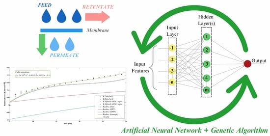
Application of Artificial Neural Networks for Modelling and Control of Flux Decline in Cross-Flow Whey Ultrafiltration

Abstract

This study is part of the re-valorisation of the dairy waste industry through the use of membrane ultrafiltration (UF), in order to recover whey proteins and remove as much water as possible from the permeate. This study aimed to predict and control the permeate flux decline in cross-flow whey UF through a step procedure, and to compare different Artificial Neural Networks (ANNs), followed by a genetic algorithm (GA), as the optimization strategy. Models were developed in Matlab^® Neural Network Toolbox. ANNs of one or two hidden layers were trained and simulated. A trial-and-error procedure identified the best network based on its performance values. The networks were trained through a selected set of experimental data obtained for lab-scale hollow-fibre membrane modules used to re-value scotta, the final waste of the dairy industry. The operating conditions considered as the input of the ANN were: operating time (t_op), sampling time (t_sample), cross-flow velocity (CFV) and transmembrane pressure (TMP), while the output of the network was exclusively the normalized permeate flux (Jn). GA optimization was carried out to the following range of operating conditions to reach the best performances and to manage the fouling effect: 225 < t_op < 300 min, 8.33 < t_sample < 15.9 min, 6.25 < CFV < 8.33 L/min, and TMP equal to 1.33 bar, otherwise it can be ignored. In fact, it has been noted that the networks with only three inputs, without TMP, predict and control Jn output better. Moreover, considering the normalized flux, it was possible to ignore some other important operating conditions, such as the membrane geometry. Consequently, the proposed general solution could also be used for other kinds of membrane applications. Finally, a hybrid approach among the ANN networks and a theoretical model was also used to better predict the resistance trend. It also returned more evident correspondence results than the ANN simulation alone, especially in the initial drop of J_n. The use of the theoretical part in the hybrid approach acts as a filter and returned the following order of significance of the operational input conditions on the resistance: t_op, t_sample, CFV and TMP.

1. Introduction

1.1. Membrane Applications in the Dairy Industry

Today, thanks to their advantages over other conventional separation methods—e.g., low-temperature operation, absence of phase transition, low energy consumption and easy scale-up—membrane applications are increasingly used in the agri-food supply chain, especially in the wastewater management processes. This is particularly true for the dairy industry, in which its use is now distributed in all stages of the supply chain, e.g., separation and fractioning of fat from milk, whey defatting, casein concentration, and bacteria removal from milk [1]. Additionally, it is significant in the recovery of waste from the dairy industry [2], especially for the whey serum—the waste produced during cheese production—and the following “scotta”—the waste produced during ricotta production [3]. Both have a high pollutant load with a COD of around 60,000–80,000 mg/L and water content of 90–94%. The remaining fractions are constituted by different whey proteins (WPs) [4,5], representing good constituents from a nutritional point of view.

Ultrafiltration (UF) represents one of the most used membrane processes in the agri-food industry, because it may be used for fractioning, concentration and purification, and the subsequent choice of the membrane unit influences the productivity of the new product.

For the dairy industry, the high amount of serum waste might suggest using a hollow-fibre membrane, with an exchange area higher than other membrane modules, but it is more subject to fouling and cleanability [6,7]. Other membrane geometries may also be used, but the productivity would be lower. In each case, fouling represents one of the main drawbacks of the membrane processes. Usually, it is thwarted through the chemical modifications of the membrane surface or the variation of the system fluid dynamics.

From this overview, there is a real need to identify and optimize the operating conditions [8] to maximize membrane performance and reduce or avoid membrane wearing due to fouling.

1.2. ANN in Membrane Technologies

A dynamic model that completely describes the UF process is not available, because the complexity of the microscale phenomena occurring inside the membrane increases the mathematical complexity of the theoretical model and they have not yet been understood. At the same time, predicting permeate flux decay seems useful to understand what occurs inside a membrane and how to prevent it.

Many researchers in the literature have already developed different artificial neural network (ANN) models of different membrane technologies. In particular, many different ANN models have been developed for the UF systems to predict and control the permeate flux [9,10,11,12,13,14,15,16,17,18] and fouling [19,20]. Each model proposed started from different input layers and has at least one output. Different types of ANNs have been used for UF, with a prevalence of multilayer perceptron (MLP) and back propagation (BP) training methods. Many of these models have many different inputs—including pH and temperature—of ceramic [15] or polyacrylonitrile (PAN) material [21].

Besides the mathematical complexity of all theoretical approaches to predict UF performance [22,23], they have three essential limitations of them: (i) the need for some experimental data for determining some input variables, which sometimes is not possible; (ii) none of these theoretical models describe the entire flux–time behaviour, but in general, they predict the steady- or the pseudo-steady-state flux; (iii) each model demonstrated its validity under special input conditions.

Instead, ANNs help to model these phenomena, starting from the experimental data and without previous knowledge about the existing physical, chemical or biological relationships between inputs and outputs of a system. Therefore, the first aim of this study was to find the best and most helpful ANN model to predict and model the permeate flux decline as much as generally possible without depending on parameters related to membrane material and geometry.

Finally, to understand if the developed ANNs may always be fine, or under what conditions, an analysis of the resistances in UF the process was carried out through a hybrid model based on a serial architecture [24]. The aim was to estimate the resistance parameter through the developed ANNs. The trend of resistance helps to understand whether or not the developed networks respond to the reality of the process.

1.3. The Genetic Algorithm as the Optimization Algorithm

The genetic algorithm (GA) was used in this study as the optimization algorithm to find the optimal values of the operating conditions in the input of the ANN model. It is a heuristic search algorithm able to generate solutions for optimization problems. GAs have some advantages over other algorithms regarding the objective or fitness function (ff). First, they require only the scalar values of ff without considering the derivatives; then, GAs handle non-linear and noisy ffs and do not impose preconditions on its trend. Another essential feature is the global research made by GA; in this way, it is more likely to arrive at or near the global optimum [25]. Moreover, the ANN-GA model has already been used to find the other optimal operating conditions of other applications [21,26,27,28,29], or for the modeling and optimizing of the nanocomposite membranes [30]. For the dairy industry, an interesting hybrid application—composed by GA and ANN—was used to understand the impact on the market of some dairy products [31]. The use of GA in this study aimed to find the optimal operating parameters in input to the different ANNs trained and simulated to better model the cross-flow UF system for dairy waste recovery.

2. Materials and Methods

2.1. Neural Network Design

McCulloch and Pitts [32] first developed ANN theory as a mathematical approach. The main structure is a “node”, similar to a human brain neuron. Generally, ANN modelling has four main steps: (i) the collection of the training data input as independent variables and the data output as dependent variables; (ii) the determination of the network architecture; (iii) the training of the network; (iv) the network simulation with new and different data input.

Different ANNs were developed in this work using Matlab^® Neural Network Toolbox (nntool) Ver. R2018a (The Mathworks Inc., Natick, MA, USA) to model cross-flow whey UF. A trial-and-error step procedure was used to choose the best ANN for the cross-flow whey UF, according to the diagram shown in Figure 1, where i represents the number of layers and n_i is the neurons in the i-th layer. In this case, the training and simulation data were collected from the experimental data obtained from a lab-scale UF unit, consisting of a hollow-fibre membrane module in polyethersulfone (PES) with a molecular weight cut-off (MWCO) of 50 kDa and an internal fibre diameter of 0.05 μm. Two types of membrane were used for the lab-scale trials. One of these trials was used for the training step of the neural network, and the other part was used to simulate the network. Trials with a membrane of 24 fibres and a length equal to 28.5 cm were used for training, while trials with a membrane of 315 fibres and a length equal to 50 cm were used for simulation. The filtration mode was always in cross-flow, while the direction of filtration and the setup configuration were different between trials, but this did not affect the ANN development. The feed solution was scotta with a concentration of around 1% (w/v) in whey proteins. Scotta was sent to the membrane inlet via a peristaltic pump (Masterflex L/S, Cole-Palmer, Easy-Load II, Model 77200-50), which set the feed flux and its direction. The concentrate was returned to the feed tank. The feed tank was in plexiglass, with a capacity of 5 L. Each data of permeate flux was read at a sampling time (t_sample) of 5 min, until the end of the trial, identified by the operating time (t_op). The end of trials was defined from the experimental strategy for the optimization of the operating conditions of the lab-scale plant. They correspond to the maximization of the permeate flux decline for the membrane units used and consequently, upon reaching the pseudo-steady state flux conditions, when the permeate flux value was essentially constant. However, the exact definition of these values is not the main objective of this work. Different transmembrane pressure (TMP) and cross-flow velocity (CFV) values were set up during the experiments, in the range from 0.5 to 5.0 bar and 10 to 5 L/min, respectively. More specifically, the sets of values were as follows: 0.5, 1.0, 1.5, 2.0, 3.0 and 5.0 bar for TMP, and 10.0, 9.4, 8.1, 7.3, 6.2 and 5.0 L/min for CFV. The volume of permeate sample was collected and measured. The permeate flux (J_p) was calculated as the ratio between the permeate volume (V_p) and the product of membrane surface (A_m) and filtration time at a given filtration time:

$$J_P=\frac{V_P}{A_m·t_{sample}}$$

(1)

To make this work’s results more general and useful to other cross-flow UF systems, the permeate flux was considered normalized, dividing each value of permeate flux at a given time for the initial value of permeate flux. In this way, it was possible to have the permeate trends and not to consider the membrane geometry as an input of the neural network.

TMP is the driving force of the UF process. It occurs due to membrane resistance and for other resistance phenomena caused by fouling and polarization. The permeate flux may also be expressed as in Equation (2), thanks to resistances in the series model.

$$J_P=\frac{TMP}{\mu ·R_{tot}}$$

(2)

where μ is the permeate viscosity and R_tot is the total resistance due to the sum of all resistances [8]. Considering the normalized permeate flux in output, TMP could be neglected as the input of the neural network.

Therefore, two different neural networks were tested: the first and second have three and four inputs, respectively. Briefly, they differ from the TMP presence in input. Both networks are tested and compared to understand the real influence of TMP in input on the process. For all networks tested, before starting with training, input data was normalized through the mapminmax() Matlab function to avoid some inputs appearing more significant than others, causing a numerical overflow due to the large or small weights.

Many different ANN architectures already exist in the literature. In this paper, the attention is focused on the characterization of ANNs starting from the way the neurons are connected: Feed Forward Neural Network (FFNN), single-layer perceptron, multilayer perceptron (MLP), radial-based network, recurrent neural networks (RNN), Elman neural network, Hopfield neural network, Jordan neural network and recurrent multi-layer neural network. Each kind of neural network has its advantages and limitations. The choice of architecture for this case study was based both on the literature already present and on the verification of the different models starting from the experimental data.

The chosen architecture was an MLP, specifically a multilayer feed-forward neural network, consisting of different layers: input, hidden and output. In this case, the information is only transmitted in the forward direction from the input layer to the hidden layer—of which there may be more than one—and then to the output layer. The number of neurons in the input and output layers is derived from the physical quantities or variables in the input and output of the process. The number of hidden layers and the neurons in each depend on the physical system’s complexity and how the ANN model wants to simplify the latter. No precise rule exists for this selection, but the trial-and-error step procedure helps to design the number of hidden layers and their neuron number [14]. The number of neurons in the hidden layers could fail the mapping between input and output parameters if these are too few or too many, causing underfitting and overfitting, respectively. In the first case, an adequate number of degrees of freedom would be lacking; in the second case, the modelling of the experimental data may cause the network training to take a long time [33].

In the FFNN network, all data inputs are interfaced with the network and then propagated through it via the weighting connections. Hence, the data output of the hidden and the output layers is calculated by internal calculations, due to the actions of the hidden and output neurons. A neuron in a hidden layer produces the neuron’s output in two steps [34]:

• Taking and multiplying some numeric inputs by adjustable parameters called weights produces weighted inputs, and adds a scalar parameter called bias or a threshold value to the result:

  $$n_j={\displaystyle \sum }_{i=1}^R\left(x_j·w_{ij}\right)+b_j$$

  (3)

  where $x_j$and $w_{ij}$ are the input signals and weights, respectively; while $b_j$ represents the threshold value or the bias term.
• The calculation of the output of the neuron by applying a transfer or “activation function” on the result, which has the net input signal $n_j$ as the argument:

  $$y_j=\phi \left(n_j\right)$$

  (4)

Some types of activation function are shown in

Table 1. List of some different more common activation functions, where S represents n_j.

Activation Function Name	Function Name in Matlab Code	Equation
Linear	purelin	$\phi =S$
Hyperbolic tangent	tansig	$\phi =\left(e^S-e^{-S}\right)/\left(e^S+e^{-S}\right)$
Log-sigmoid	logsig	$\phi =1/\left(1+e^{-S}\right)$
Radial basis	radbas	$\phi =e^{-(S^2)}$
Triangular basis	tribas	$\phi =\left\{\begin{array}{c}1-\left|S\right|, 1\le S\le 1\\ 0, S\le -1 or S\ge 1 \end{array}\right.$

. In this paper, the hyperbolic tangent function (tansig) was used for the hidden layer(s), while the linear function (purelin) was used for the output function. The output obtained $y_j$ is compared with the corresponding target t_j, and from the difference between them, different error functions may be calculated and the ANN performance can be measured. In this work, Mean Square Error (MSE) and the correlation coefficient (R) were selected to evaluate network performance. In particular, MSE was also used in the optimization step.

$$MSE=\frac{1}{\mathrm{N}}{\displaystyle \sum }_{\mathrm{i}=1}^{\mathrm{N}}{\left({\mathrm{X}}_{\mathrm{experimental}\left(\mathrm{i}\right)}-{\mathrm{X}}_{\mathrm{calculated}\left(\mathrm{i}\right)}\right)}^2$$

(5)

$$R={\left[1-\frac{{{\displaystyle \sum }}_{\mathrm{i}=1}^{\mathrm{N}}{\left({\mathrm{X}}_{\mathrm{experimental}\left(\mathrm{i}\right)}-{\mathrm{X}}_{\mathrm{calculated}\left(\mathrm{i}\right)}\right)}^2}{{{\displaystyle \sum }}_{\mathrm{i}=1}^{\mathrm{N}}{\left({\mathrm{X}}_{\mathrm{experimental}\left(\mathrm{i}\right)}-\overline{{\mathrm{X}}_{\mathrm{experimental}}}\right)}^2}\right]}^{1/2}$$

(6)

where ${\mathrm{X}}_{\mathrm{experimental}\left(\mathrm{i}\right)}$ and ${\mathrm{X}}_{\mathrm{calculated}\left(\mathrm{i}\right)}$ are the i-th experimental and calculated values, while $\overline{{\mathrm{X}}_{\mathrm{experimental}}}$ is the mean of the experimental values. N is the number of the data point.

Regarding the training algorithms, the most popular and successful—also for similar applications to this case study—seems to be the back-propagation algorithm [35]. It is based on the steepest-descent principle. Back propagation performs supervised learning in which the network is trained by implementing data for which input vectors are known and a target is associated with each input vector [36].

By using the nntool command in Matlab, it was possible to import, create, use and export neural networks and data. Moreover, through a Matlab string command genFunction(), it was possible to generate a valuable Matlab code function for the subsequent simulation and optimization phase of the network. It was possible to modify the generated network in all its parts after it was created and then modify it in the final optimized configuration for this application.

2.2. A Hybrid Serial Architecture Model for the Evaluation of Resistances

As a rule, the main use of a hybrid model of a system is to describe some well-evaluated phenomena through theoretical relationships, leaving the analysis of other aspects, which are generally difficult to interpret, to the neural networks. The theoretical part of a hybrid structure may perform as a filter function that can limit the error propagation even when the inputs are perturbed. A serial architecture of the hybrid model lets us use the normalized permeate flux in the output of the network as the input of the theoretical model to evaluate the transport resistances in the UF membrane system and whether or not they are comparable and acceptable to the real UF system. The theoretical part of the model comes from the balance of whey proteins—whose concentration is known from the experimental data—the balance on the lab-scale system in batch conditions [37] and the series resistance model expressed in Equation (2). From these, the normalized permeate flux in the theoretical model may be expressed as in Equation (7):

$$J_n=1-\frac{K}{TMP}·\frac{CFV·t_{op}-V_0}{t_{op}-t_{sample}}$$

(7)

where K is the resistance factor, expressed in Equation (8). It contains the dependency of membrane geometry and the flow viscosity which passes through the membrane, besides the resistance trend. At the start, it may also be estimated from the whey proteins’ balance. K is expressed in $bar·\min ·{\mathrm{m}}^{-3}$.

$$K=\frac{\mu ·R_{TOT}}{A_m}$$

(8)

Not considering the membrane properties and the flow that crosses it, K may be obtained from Equation (7), starting from the neural network output and the boundary constraints in

Table 2. Boundary constraints for the Genetic Algorithm optimization.

Boundary Constraints	Operating Time top (min)	Sampling Time tsample (min)	Cross-Flow Velocity CFV (L/min)	Transmembrane Pressure TMP (bar)
Lower	30	5	5	0.5
Upper	330	30	10	5

. These values were compared to the K coming from the experimented data set also used for the simulation step.

$$K=\left(1-J_n\right)·\frac{TMP·\left(t_{op}-t_{sample}\right)}{CFV·t_{op}-V_0}$$

(9)

Thanks to this hybrid approach, it was also possible to investigate what variable most influences the permeate flux trend, and at the same time, the resistance trend.

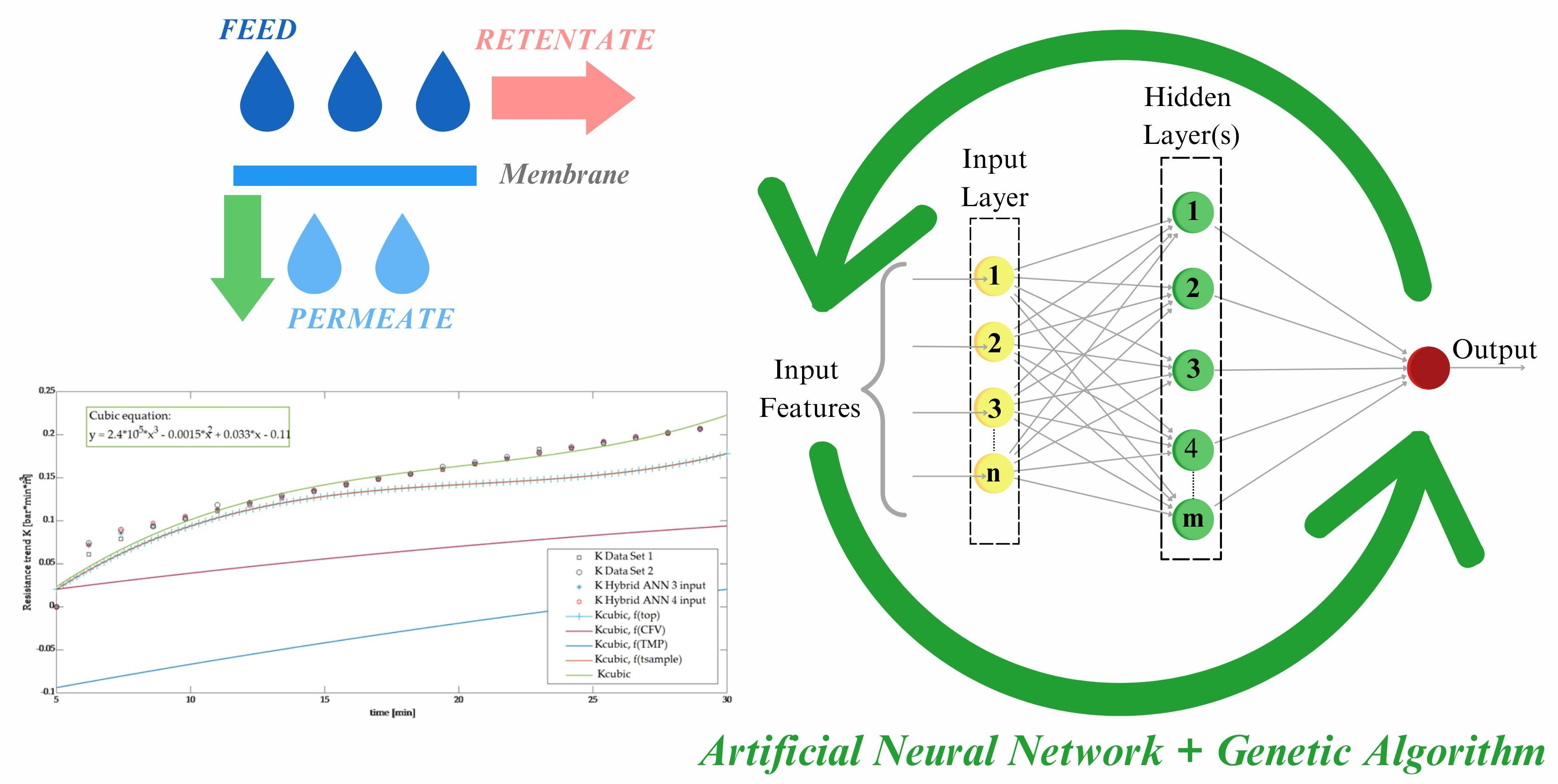
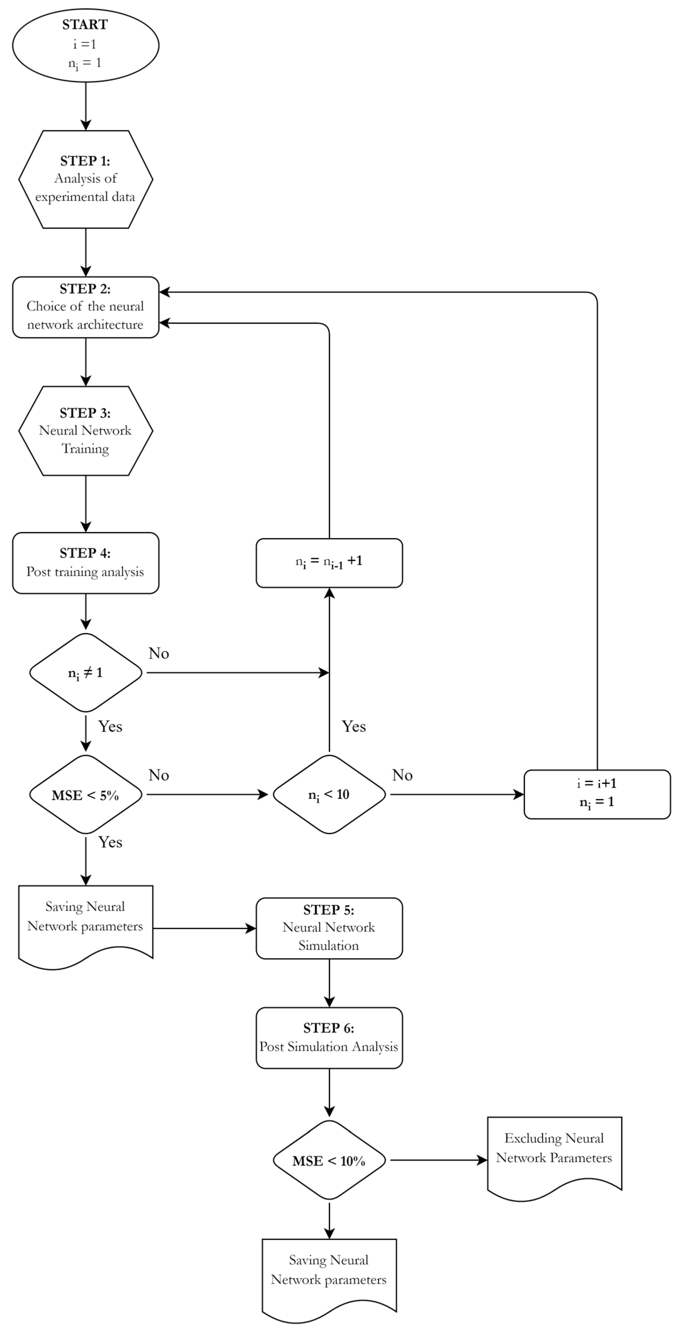
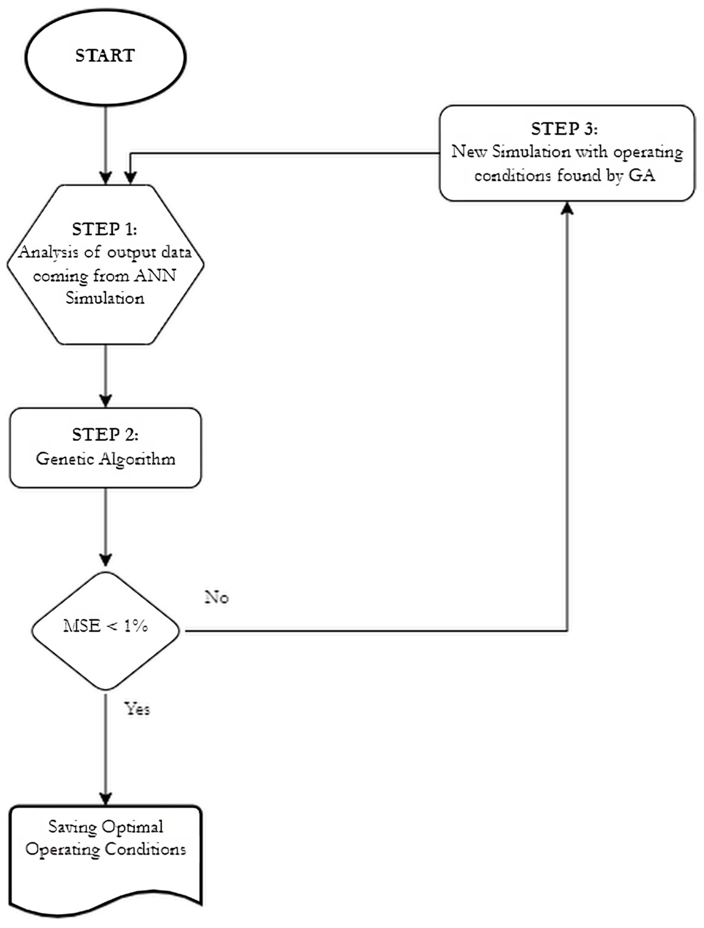
2.3. Neural Network Optimization

The optimization step consists of optimising the input variables of the neural networks to minimize or maximize the output variable. In this study, a GA was used to optimize the normalized flux decline. By using the optimization Matlab tool (optimtool), it was possible to set up the optimization phase according to the diagram shown in Figure 2.

The fitness function used for the GA was the MSE, which was calculated for each iteration of the simulation phase for each network analyzed. If MSE was lower than 1%, the operating conditions found by the algorithm were then saved as optimal operating conditions for the network. Otherwise, the operating conditions found were then used as the new input for the network simulation.

For the GA operation, a hybrid function was used to find a minimum constrained nonlinear multivariable function (fmincon), within the bound constraints due, in this case, to the physics of the system. The bound constraints were set up as an array with minimum and maximum values of the input variables of the neural networks, as shown in Table 2.

3. Results

After developing the networks, it was necessary to measure their performances. According to the previous trial-and-error step procedure, the performance of the ANNs was evaluated through MSE and R. In the following subsections, the performances of the main ANNs of interest are shown for networks with three and four inputs.

The other subsections regard evaluating the resistance trend using a hybrid model and the optimization results obtained with the genetic algorithm.

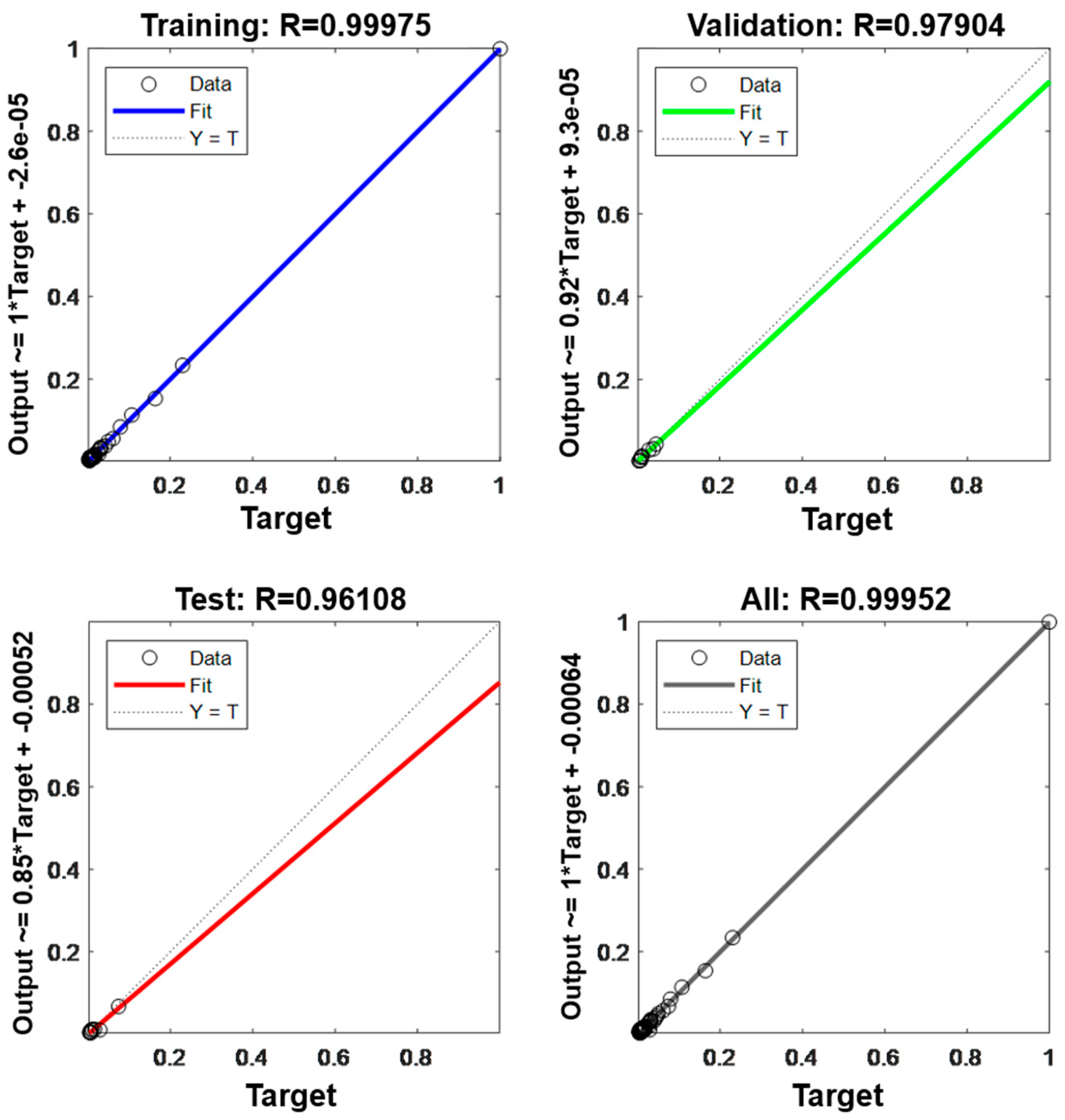
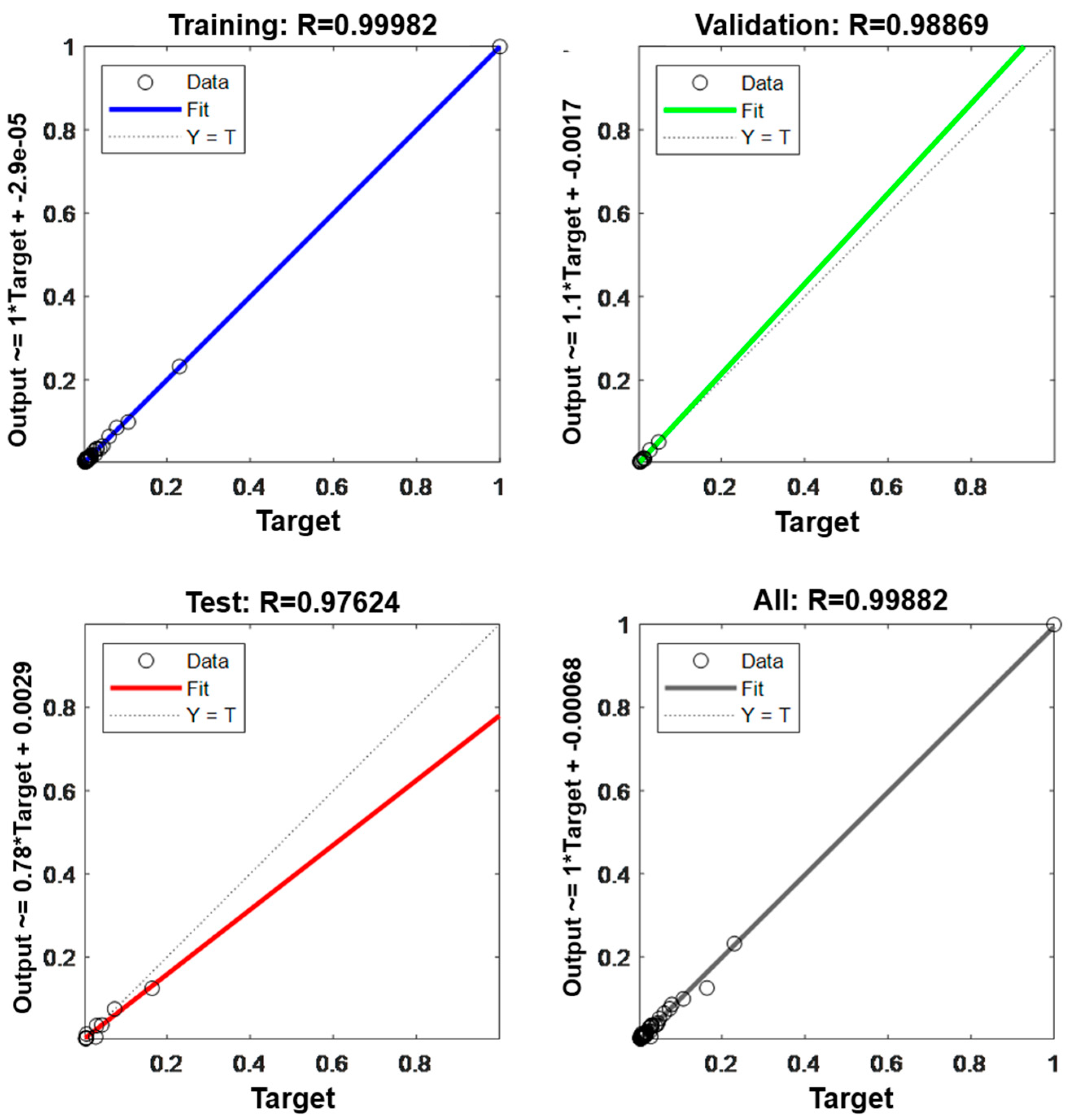
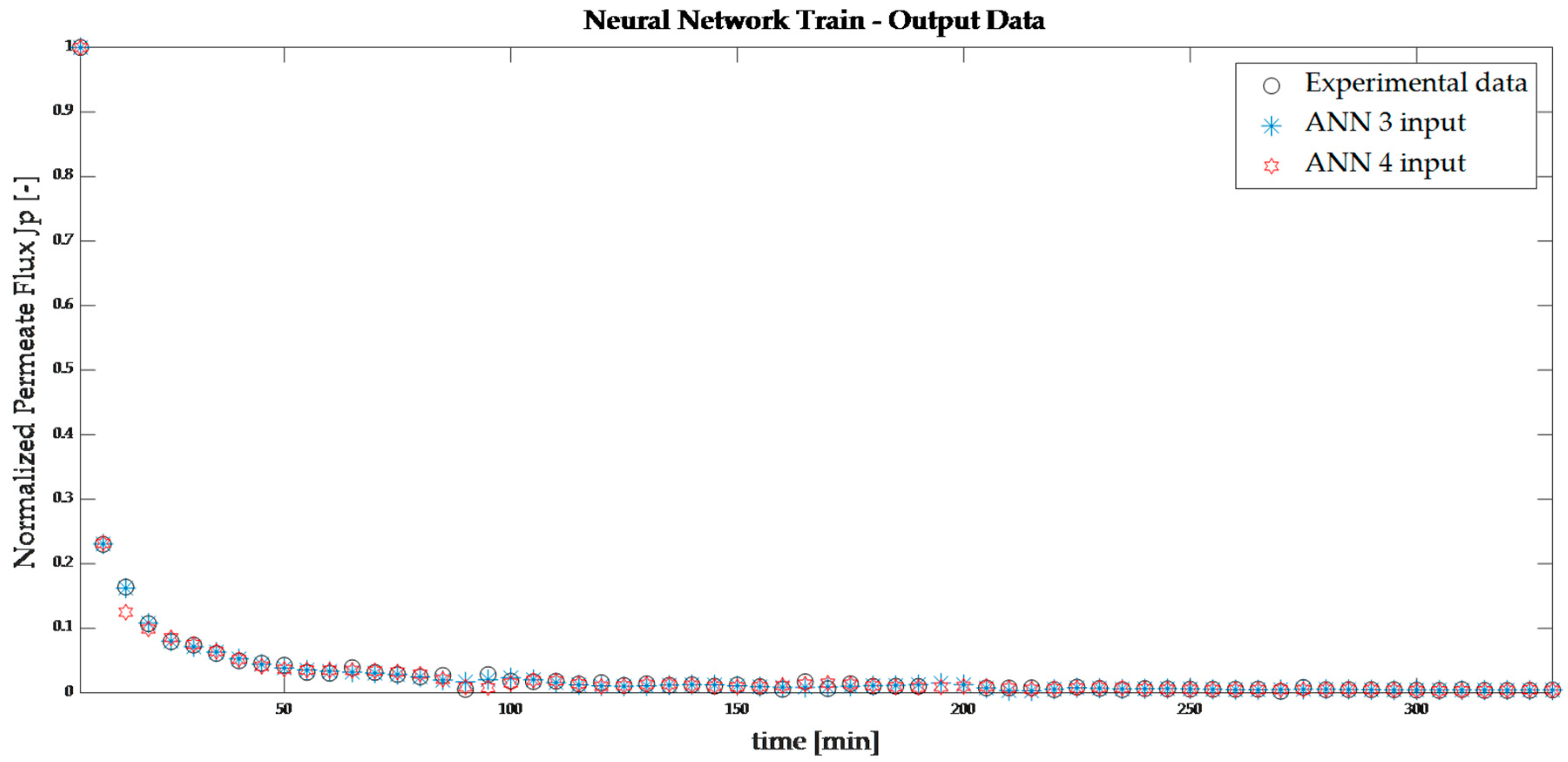
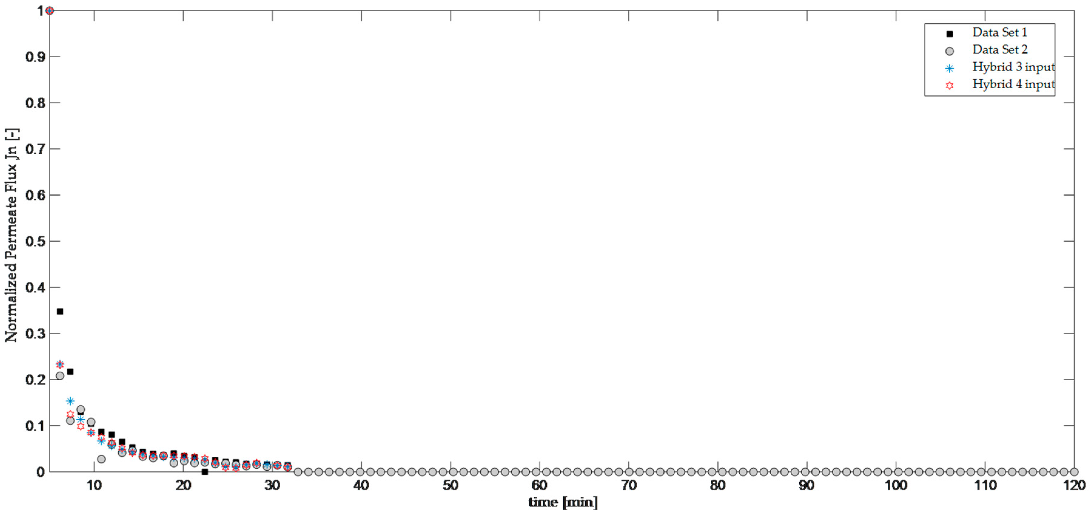
3.1. ANN Model Performance

Table 3. ANN architectures and their performance for a network with three inputs.

Scenario	Neurons in Hidden Layer 1	Neurons in Hidden Layer 2	MSE	Training Performance	Validation Performance	Test Performance	R
1	6	6	2.40 × 10−3	3.11 × 10−3	1.40 × 10−3	6.63 × 10−1	0.95676
2	7	7	2.64 × 10−5	2.82 × 10−5	1.42 × 10−1	2.89 × 10−1	0.99918
3	8	0	1.30 × 10−3	3.43 × 10−5	1.30 × 10−3	4.22 × 10−5	0.99274
4	8	8	1.60 × 10−5	1.10 × 10−5	1.10 × 10−5	4.66 × 10−5	0.99952
5	8	9	5.42 × 10−4	7.54 × 10−4	3.14 × 10−5	5.05 × 10−5	0.98395
6	8	10	1.52 × 10−4	1.94 × 10−4	3.11 × 10−5	7.02 × 10−1	0.99759
7	9	9	1.09 × 10−4	1.15 × 10−4	4.83 × 10−1	1.43	0.99854
8	10	10	2.44 × 10−5	2.34 × 10−5	4.50 × 10−1	1.09 × 10−1	0.99924

and

Table 4. ANN architectures and their performance for a network with four inputs.

Scenario	Neurons in Hidden Layer 1	Neurons in Hidden Layer 2	MSE	Training Performance	Validation Performance	Test Performance	R
1	8	0	4.09 × 10−2	1.63 × 10−5	4.09 × 10−2	1.49 × 10−5	0.89667
2	8	8	2.91 × 10−4	3.76 × 10−4	1.35 × 10−4	3.58 × 10−5	0.99239
3	8	9	2.81 × 10−4	7.49 × 10−6	8.26 × 10−6	1.76 × 10−3	0.99233
4	8	10	5.29 × 10−4	1.16 × 10−5	3.68 × 10−3	6.03 × 10−5	0.98350
5	9	0	7.15 × 10−4	9.85 × 10−4	1.81 × 10−4	6.11 × 10−5	0.97828
6	9	9	3.88 × 10−5	8.07 × 10−6	6.06 × 10−6	2.07 × 10−4	0.99882
7	10	0	1.02 × 10−4	1.40 × 10−4	8.58 × 10−6	2.81 × 10−5	0.99720
8	10	10	5.38 × 10−4	7.28 × 10−4	2.88 × 10−5	1.40 × 10−4	0.98433

summarize the network hidden layers architecture developed through the trial-and-error step procedure with three and four input variables. The most significant performances in terms of MSE for each training, validation and test phase within the R values are also presented in the same tables. MSE and R take on values between 0 and 1. An MSE close to 0, indicates a high precision of the ANN. On the contrary, a high value of R, usually close to 1, indicates a more useful model. Figure 3 and Figure 4 show the overall values of R within the R for each training validation and test phase for the network identified as performing the best in the post-training analysis.

For both the networks with three and four input variables, the best performances in post-training analysis were given by the network with two hidden layers. In particular, for networks with three input variables, the best network was identified with eight neurons for each hidden layer; while for networks with four input variables, the best network identified had nine neurons for each hidden layer.

These networks were simulated with two other different experimental data sets. The MSE performances are also presented in

Table 5. ANN architectures and their performance for the simulation step.

Neurons in the Input Layer	Neurons in Hidden Layer 1	Neurons in Hidden Layer 2	Data Set	MSE
3	8	8	1	0.035
3	8	8	2	0.005
4	9	9	1	0.042
4	9	9	2	0.002

for two different data sets. These experimental data sets come from different hollow-fibre membrane systems. The first and the second data set contain 258 and 200 data points, respectively. The setup division for data training, validation and testing phases consists of 70%, 15% and 15% of the entire datasets, respectively. The first was installed in a horizontal configuration and had an In-to-Out filtration mode. In contrast, the second was installed in a vertical configuration and had an Out-to-In filtration mode. It was experimentally demonstrated that the first system had a greater tendency to cause fouling than the second [3].

From the performance values, the best ANN results for the network with three inputs are for the network with two layers and eight neurons each. The best ANN results for the network with four inputs are for the network with two layers and nine neurons each.

The normalized permeate flux predicted in the post-training and post simulation analyses are compared with the experimental data in Figure 5 and Figure 6.

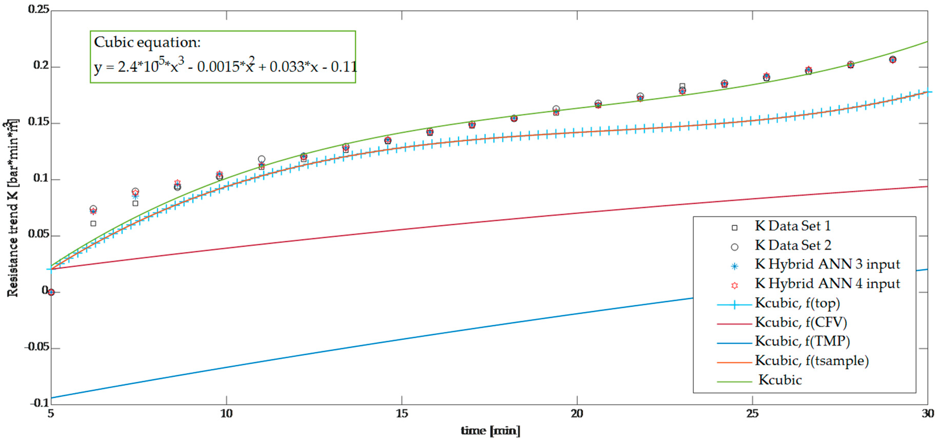
3.2. K-Resistance Trends from the Hybrid Model

The comparisons between the normalized permeate flux trends calculated from the evaluation of K from the theoretical model shown in Figure 7 show substantial correspondence between the experimental flow trends, unlike with the use of only the neural network, as in Figure 6. The correspondence results are much more evident than the ANN simulation results, especially in the initial rapid drop. Thus, analyzing the K-trends may provide more information about the variable’s dependence with the permeate flux. Figure 8 presents the K-trend for both experimental and hybrid cases. They try to provide a K-trend expressed by only one variable through a cubic interpolation. The cubic interpolation seems to be the best kind of interpolation among the simpler ones, and it is the only one showing a comparable trend from the different input variables.

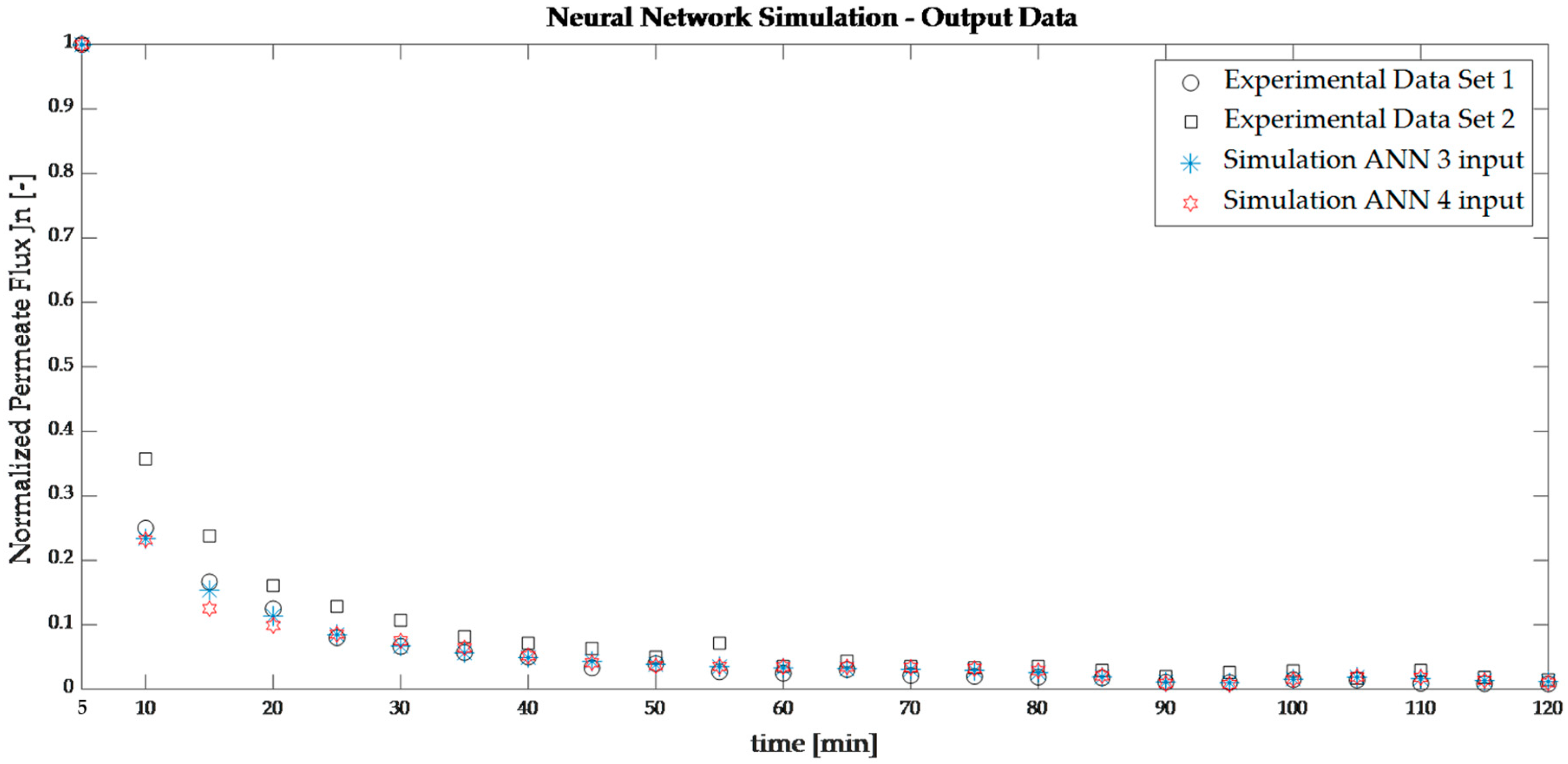
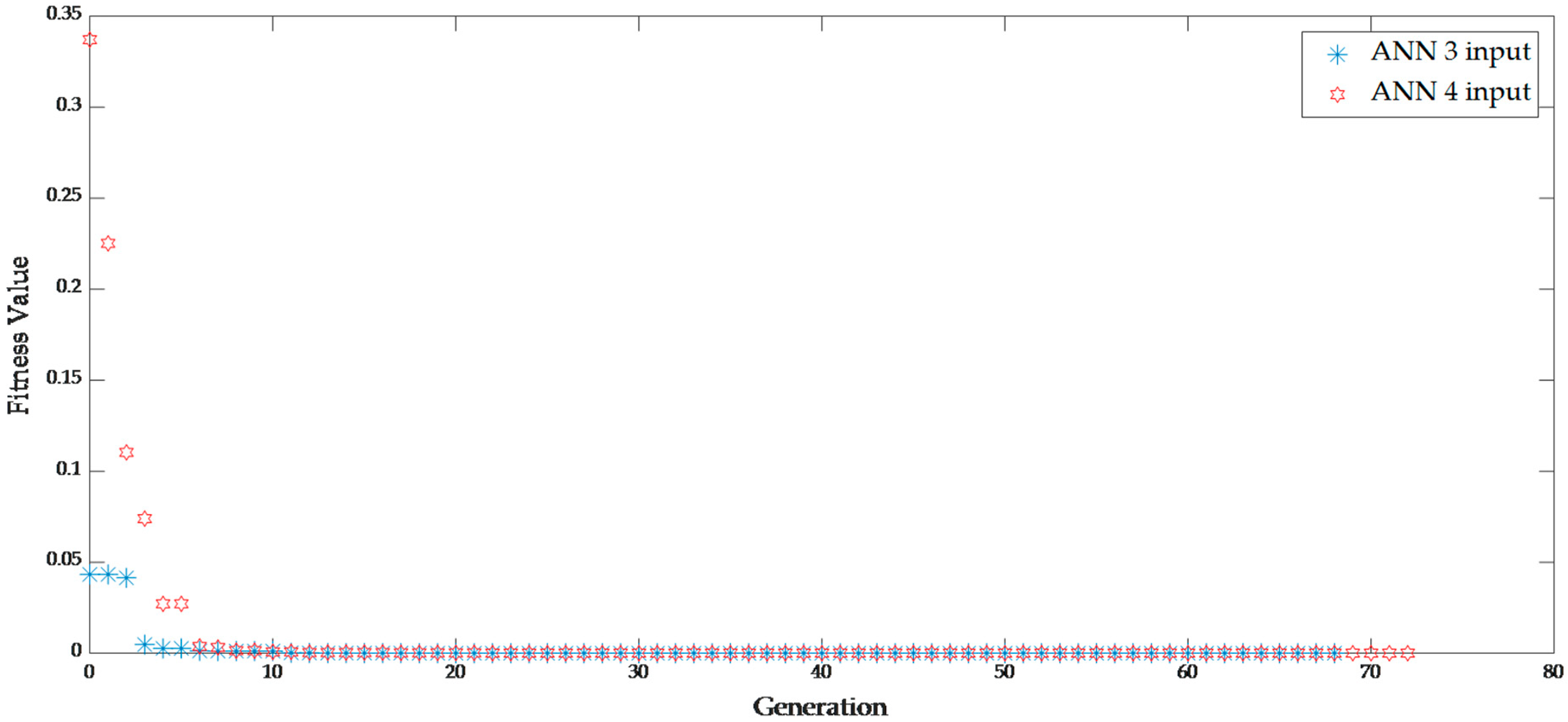
3.3. Optimization Results

The optimization results show the minimum raised to the ANNs simulated and optimized through the genetic algorithm with MSE as the fitness function. In Figure 9, the MSE trends for both the ANNs are presented. In both optimization cases, the optimization process results are completed because the fitness function did not decrease in feasible directions to within the value of the optimal tolerance; moreover, the constraints are satisfied to within the value of the constraint tolerance.

Table 6. Optimal performance and operating conditions for both ANNs developed.

ANN Inputs	Minimum MSE	Optimal Operating Conditions
		Operating Time top (min)	Sampling Time tsample (min)	Cross-Flow Velocity CFV (L/min)	Transmembrane Pressure TMP (bar)	Normalized Permeate Flux (%)
3	2.89 × 10−13	300	8.33	8.33	-	1.00
4	1.71 × 10−11	225	15.9	6.25	1.33	7.41

presents the optimization results in terms of minimum MSE value and optimal operating conditions to ensure a maximum decay of permeate flux in output to the UF process.

4. Discussion

Post-training and post-simulation analysis show a few differences, especially in the initial rapid drop of the permeate flux, for both ANNs. Cross-flow whey UF is a physical system subject to fouling, biological phenomena due to the presence of proteins and other micro-scale phenomena. It may produce different results when modifying the operating conditions or replacing the membrane with others with different physical characteristics. However, the simulation step shows excellent performance, especially for the experimental data obtained with a UF system installed in a vertical configuration and an Out-to-In filtration mode. At the same time, the ANN with three input variables showed a slightly better performance with the first experimental data set obtained with a UF system installed in a horizontal mode and an In-to-Out filtration mode, such as the data set used for the training step. Data set 1 showed a higher tendency for fouling than data set 2.

The use of the hybrid model for this system, given by the set of the theoretical model and the neural network, shows better accordance with both experimental data than with neural networks alone. Moreover, K-trends with a cubic interpolation indicate the influence that the various operating variables have on the permeate flux and, thus, on the resistance to transport given mainly by fouling, and other eventual concentration polarisation phenomena. Figure 8 clearly shows that K has the most influence in the time variables. Looking at Equation (9) regarding the theoretical model, it is easy to imagine that the filtration time has a much higher influence than the sampling time. Cross-flow velocity presents a more minor influence than time variables, while transmembrane pressure shows a minor influence, even with initial negative K values. This would also explain the comparable performance of the neural networks developed with three and four inputs under some specific conditions. As the permeate flux directly proportional to K, it presents the same dependencies with K.

The optimization results obtained with the genetic algorithm show the optimal operating conditions to obtain the maximum decay of the permeate flux, which is useful to remove the maximum amount of water from the dairy waste and ensure its re-valorisation. The network with three inputs seems to have the best results in terms of performance. In this case, transmembrane pressure may be neglected, and it can consider a function of the cross-flow velocity. The neural network with four inputs still performs excellently and identifies an optimum value of transmembrane pressure. It is very close to the true optimal value obtained experimentally in the lab. The interval between the optimal conditions of the input variables of both models may represent the range for the experimental operating conditions to reach the best performance and to manage the fouling effect.

5. Conclusions

In this study, different prediction models of the permeate flux decline were developed to model and control cross-flow whey ultrafiltration. Both the developed ANN models developed showed a good fit with the experimental data. Comparing the lab-experimental conditions with the ANN results, it can be seen that the ANN with three input variables is more suitable for a high membrane exchange area. In this case, the transmembrane pressure could be neglected because it can reach minimal values; while cross-flow velocity can achieve higher values. The ANN with four input variables is more suitable for a lower membrane area, with higher transmembrane pressure values and, consequently, lower values of cross-flow velocity.

A hybrid model was developed to understand the real influence of the input variables on the permeate flux in the output of the UF system and understand if the ANN models are reliable, starting from a theoretical part of the system passing through the neural network. The main advantage of a hybrid model is the possibility of describing some well-evaluated phenomena from theoretical relationships, leaving the analysis of various aspects which are generally challenging to evaluate in neural networks. Thus, the presence of a hybrid structure also significantly improves the neural network model. This is mainly due to the theoretical part, which performs as a filter limiting the error propagation in the system. A serial architecture was used for the hybrid model development: the process output variable—difficult to measure and predict without the geometry and the specific operating conditions—is estimated by a neural network model and then fed as the input of the theoretical relationship. Through this hybrid model, a K-resistance trend was evaluated. The presence of the theoretical part greatly reduced the differences between the neural models, acting as a filter. A cubic interpolation was then performed to evaluate the significance of the operational input conditions on the permeation flux. It returned the following order: operating time (t_op), sampling time (t_sample), cross-flow velocity (CFV) and finally, transmembrane pressure (TMP). This result is the optimization step developed with the genetic algorithm. This optimization returned excellent performances for both networks. The identified operating conditions for both neural network models may represent the range of the experimental operating conditions: 225 < t_op < 300 min, 8.33 < t_sample < 15.9 min, 6.25 < CFV < 8.33 L/min, TMP is equal to 1.33 bar, otherwise it can be neglected.

References

1. Reig, M.; Vecino, X.; Cortina, J.L. Use of Membrane Technologies in Dairy Industry: An Overview. Foods 2021, 10, 2768. [Google Scholar] [CrossRef] [PubMed]
2. Papaioannou, E.H.; Mazzei, R.; Bazzarelli, F.; Piacentini, E.; Giannakopoulos, V.; Roberts, M.R.; Giorno, L. Agri-Food Industry Waste as Resource of Chemicals: The Role of Membrane Technology in Their Sustainable Recycling. Sustainbility 2022, 14, 1483. [Google Scholar] [CrossRef]
3. Gaudio, M.T.; Curcio, S.; Chakraborty, S. Design of an Integrated Membrane System to Produce Dairy By-Product from Waste Processing. Int. J. Food Sci. Technol. 2023, 58, 2104–2114. [Google Scholar] [CrossRef]
4. Ramos, O.L.; Pereira, R.N.; Rodrigues, R.M.; Teixeira, J.A.; Vicente, A.A.; Malcata, F.X. Whey and Whey Powders: Production and Uses. In Encyclopedia of Food and Health; Elsevier Inc.: Amsterdam, The Netherlands, 2015; pp. 498–505. ISBN 9780123849533. [Google Scholar]
5. Monti, L.; Donati, E.; Zambrini, A.V.; Contarini, G. Application of Membrane Technologies to Bovine Ricotta Cheese Exhausted Whey (Scotta). Int. Dairy J. 2018, 85, 121–128. [Google Scholar] [CrossRef]
6. Castro, B.N.; Gerla, P.E. Hollow Fiber and Spiral Cheese Whey Ultrafiltration: Minimizing Controlling Resistances. J. Food Eng. 2005, 69, 495–502. [Google Scholar] [CrossRef]
7. Daufin, G.; Escudier, J.P.; Carrère, H.; Bérot, S.; Fillaudeau, L.; Decloux, M. Recent and Emerging Applications of Membrane Processes in the Food and Dairy Industry. Food Bioprod. Process. Trans. Inst. Chem. Eng. Part C 2001, 79, 89–102. [Google Scholar] [CrossRef]
8. Cui, Z.F.; Jiang, Y.; Field, R.W. Fundamentals of Pressure-Driven Membrane Separation Processes. In Membrane Technology; Elsevier Ltd.: Amsterdam, The Netherlands, 2010; pp. 1–18. ISBN 9781856176323. [Google Scholar]
9. Niemi, H.; Bulsari, A.; Palosaari, S. Simulation of Membrane Separation by Neural Networks. J. Memb. Sci. 1995, 102, 185–191. [Google Scholar] [CrossRef]
10. Razavi, M.A.; Mortazavi, A.; Mousavi, M. Dynamic Modelling of Milk Ultrafiltration by Artificial Neural Network. J. Memb. Sci. 2003, 220, 47–58. [Google Scholar] [CrossRef]
11. Rai, P.; Majumdar, G.C.; DasGupta, S.; De, S. Modeling the Performance of Batch Ultrafiltration of Synthetic Fruit Juice and Mosambi Juice Using Artificial Neural Network. J. Food Eng. 2005, 71, 273–281. [Google Scholar] [CrossRef]
12. Curcio, S.; Calabrò, V.; Iorio, G. Reduction and Control of Flux Decline in Cross-Flow Membrane Processes Modeled by Artificial Neural Networks. J. Memb. Sci. 2006, 286, 125–132. [Google Scholar] [CrossRef]
13. Chen, H.; Kim, A.S. Prediction of Permeate Flux Decline in Crossflow Membrane Filtration of Colloidal Suspension: A Radial Basis Function Neural Network Approach. Desalination 2006, 192, 415–428. [Google Scholar] [CrossRef]
14. Sarkar, B.; Sengupta, A.; De, S.; DasGupta, S. Prediction of Permeate Flux during Electric Field Enhanced Cross-Flow Ultrafiltration—A Neural Network Approach. Sep. Purif. Technol. 2009, 65, 260–268. [Google Scholar] [CrossRef]
15. Guadix, A.; Zapata, J.E.; Almecija, M.C.; Guadix, E.M. Predicting the Flux Decline in Milk Cross-Flow Ceramic Ultrafiltration by Artificial Neural Networks. Desalination 2010, 250, 1118–1120. [Google Scholar] [CrossRef]
16. Madaeni, S.S.; Hasankiadeh, N.T.; Tavakolian, H.R. Modeling and Optimization of Membrane Chemical Cleaning by Artificial Neural Network, Fuzzy Logic, and Genetic Algorithm. Chem. Eng. Commun. 2012, 199, 399–416. [Google Scholar] [CrossRef]
17. Yangali-Quintanilla, V.; Verliefde, A.; Kim, T.U.; Sadmani, A.; Kennedy, M.; Amy, G. Artificial Neural Network Models Based on QSAR for Predicting Rejection of Neutral Organic Compounds by Polyamide Nanofiltration and Reverse Osmosis Membranes. J. Memb. Sci. 2009, 342, 251–262. [Google Scholar] [CrossRef]
18. Rahmanian, B.; Pakizeh, M.; Mansoori, S.A.A.; Esfandyari, M.; Jafari, D.; Maddah, H.; Maskooki, A. Prediction of MEUF Process Performance Using Artificial Neural Networks and ANFIS Approaches. J. Taiwan Inst. Chem. Eng. 2012, 43, 558–565. [Google Scholar] [CrossRef]
19. Soleimani, R.; Shoushtari, N.A.; Mirza, B.; Salahi, A. Experimental Investigation, Modeling and Optimization of Membrane Separation Using Artificial Neural Network and Multi-Objective Optimization Using Genetic Algorithm. Chem. Eng. Res. Des. 2013, 91, 883–903. [Google Scholar] [CrossRef]
20. Delgrange, N.; Cabassud, C.; Cabassud, M.; Durand-Bourlier, L.; Lainé, J.M. Modelling of Ultrafiltration Fouling by Neural Network. Desalination 1998, 118, 213–227. [Google Scholar] [CrossRef]
21. Badrnezhad, R.; Mirza, B. Modeling and Optimization of Cross-Flow Ultrafiltration Using Hybrid Neural Network-Genetic Algorithm Approach. J. Ind. Eng. Chem. 2014, 20, 528–543. [Google Scholar] [CrossRef]
22. Cheryan, M.; Cheryan, M. Ultrafiltration and Microfiltration Handbook; Technomic Pub. Co.: Lancaster, PA, USA, 1998; ISBN 9781566765985. [Google Scholar]
23. Samuelsson, G.; Huisman, I.H.; Trägårdh, G.; Paulsson, M. Predicting Limiting Flux of Skim Milk in Crossflow Microfiltration. J. Memb. Sci. 1997, 129, 277–281. [Google Scholar] [CrossRef]
24. Saraceno, A.; Curcio, S.; Calabrò, V.; Iorio, G. A Hybrid Neural Approach to Model Batch Fermentation of “Ricotta Cheese Whey” to Ethanol. Comput. Chem. Eng. 2010, 34, 1590–1596. [Google Scholar] [CrossRef]
25. Sivanandam, S.N.; Deepa, S.N. Genetic Algorithms. Introd. to Genet. Algorithms 2008. [Google Scholar] [CrossRef]
26. Chow, T.T.; Zhang, G.Q.; Lin, Z.; Song, C.L. Global Optimization of Absorption Chiller System by Genetic Algorithm and Neural Network. Energy Build. 2002, 34, 103–109. [Google Scholar] [CrossRef]
27. Madaeni, S.S.; Hasankiadeh, N.T.; Kurdian, A.R.; Rahimpour, A. Modeling and Optimization of Membrane Fabrication Using Artificial Neural Network and Genetic Algorithm. Sep. Purif. Technol. 2010, 76, 33–43. [Google Scholar] [CrossRef]
28. Reihanian, M.; Asadullahpour, S.R.; Hajarpour, S.; Gheisari, K. Application of Neural Network and Genetic Algorithm to Powder Metallurgy of Pure Iron. Mater. Des. 2011, 32, 3183–3188. [Google Scholar] [CrossRef]
29. Cong, T.; Su, G.; Qiu, S.; Tian, W. Applications of ANNs in Flow and Heat Transfer Problems in Nuclear Engineering: A Review Work. Prog. Nucl. Energy 2013, 62, 54–71. [Google Scholar] [CrossRef]
30. Arefi-Oskoui, S.; Khataee, A.; Vatanpour, V. Modeling and Optimization of NLDH/PVDF Ultrafiltration Nanocomposite Membrane Using Artificial Neural Network-Genetic Algorithm Hybrid. ACS Comb. Sci. 2017, 19, 464–477. [Google Scholar] [CrossRef] [PubMed]
31. Goli, A.; Zare, H.K.; Moghaddam, R.; Sadeghieh, A. A Comprehensive Model of Demand Prediction Based on Hybrid Artificial Intelligence and Metaheuristic Algorithms: A Case Study in Dairy Industry. SSRN Electron. J. 2018, 11, 190–203. [Google Scholar]
32. McCulloch, W.S.; Pitts, W. A Logical Calculus of the Ideas Immanent in Nervous Activity. Bull. Math. Biophys. 1943, 5, 115–133. [Google Scholar] [CrossRef]
33. Mohammadi, A.H.; Belandria, V.; Richon, D. Use of an Artificial Neural Network Algorithm to Predict Hydrate Dissociation Conditions for Hydrogen+water and Hydrogen+tetra-n-Butyl Ammonium Bromide+water Systems. Chem. Eng. Sci. 2010, 65, 4302–4305. [Google Scholar] [CrossRef]
34. Alamolhoda, S.; Kazemeini, M.; Zaherian, A.; Zakerinasab, M.R. Reaction Kinetics Determination and Neural Networks Modeling of Methanol Dehydration over Nano γ-Al2O3 Catalyst. J. Ind. Eng. Chem. 2012, 18, 2059–2068. [Google Scholar] [CrossRef]
35. Istadi, I.; Amin, N.A.S. Modelling and Optimization of Catalytic–Dielectric Barrier Discharge Plasma Reactor for Methane and Carbon Dioxide Conversion Using Hybrid Artificial Neural Network—Genetic Algorithm Technique. Chem. Eng. Sci. 2007, 62, 6568–6581. [Google Scholar] [CrossRef]
36. Lahiri, S.K.; Ghanta, K.C. Development of an Artificial Neural Network Correlation for Prediction of Hold-up of Slurry Transport in Pipelines. Chem. Eng. Sci. 2008, 63, 1497–1509. [Google Scholar] [CrossRef]
37. Green, D.W.; Perry, R.H. Perry’s Chemical Engineers’ Handbook, 8th ed.; McGraw-Hill Education: New York, NY, USA, 2008; ISBN 9780071422949. [Google Scholar]
Figure 1. Artificial Neural Network trial-and-error step procedure.
Processes 11 01287 g001
Figure 2. Optimization strategy of the input parameters.
Processes 11 01287 g002
Figure 3. The correlation coefficient R for training analysis of an ANN with three variables in the input layer, and two hidden layers with eight neurons each.
Processes 11 01287 g003
Figure 4. The correlation coefficient R for training analysis of an ANN with four variables in the input layer, and two hidden layers with nine neurons each.
Processes 11 01287 g004
Figure 5. Post training analysis—comparison between experimental data and ANNs developed with three and four inputs.
Processes 11 01287 g005
Figure 6. Post simulation analysis—comparison between both experimental data sets used in the simulation phase and ANNs developed with three and four inputs.
Processes 11 01287 g006
Figure 7. Comparison between the normalized permeate flux from both experimental data sets and the normalized permeate flux from the hybrid model from the theoretical approach and the ANNs developed with three and four inputs.
Processes 11 01287 g007
Figure 8. K-resistance trends, both experimental and hybrid. The cubic interpolation between them and the dependency of each variable with cubic K.
Processes 11 01287 g008
Figure 9. Trends of MSE for both ANNs optimized through a GA.
Processes 11 01287 g009