Saturation Determination and Fluid Identification in Carbonate Rocks Based on Well Logging Data: A Middle Eastern Case Study

Abstract

In the Middle East, there remain many technical challenges in the water saturation evaluation of carbonate rocks and the effective identification of reservoir fluid properties. The traditional Archie equation is not applicable to carbonate reservoirs with complex pore structures and varying reservoir space distribution, as there are obvious “non-Archie” phenomena. In this paper, by analyzing the experimental data on the rock resistivity of the target formation in the study area and analyzing the relationship between stratigraphic factors and porosity, the previous fitting method was modified as a result of using the actual data while avoiding the cementation index as a way to improve Archie’s formula to evaluate the water saturation. Based on the improved Archie formula, the mathematical differential operation of water saturation and porosity was carried out using the formation resistivity. The calculation results of irreducible water saturation were used to calibrate the oil layer, and the water layer was calibrated when the water saturation was 100%, allowing for a novel reservoir fluid property identification method. This total differential method can effectively identify the oil-down-to (ODT) and water-up-to (WUT) levels in an oil–water system and then accurately divide the transition zone of the oil–water layer. When this method was applied, the identification results were in good agreement with production conclusions and test data with an accuracy rate of 89.95%. Although the use of geophysical logging data from open-hole wells combined with the total differential method is only applicable to wells with similar logging time and production time, it is possible to compare geophysical logging data from different periods to construct oil–water profiles to observe the changes in ODT over time to guide development and adjust production plans. The proposed reservoir fluid property identification method and the improved water saturation calculation formula can meet the requirements of water saturation evaluation in the target block with low calculation cost and easy implementation, which provides a new method for water saturation evaluation and rapid identification of reservoir fluid properties.

1. Introduction

Oil and gas resources in carbonate rocks are abundant, accounting for more than 60% of the world’s remaining oil and gas resources [1,2]. The Middle East is extremely rich in oil resource production, mostly from carbonate oil and gas fields, which has led to an increase in the exploration of carbonate oil and gas reservoirs in this area by major oil companies [3]. Most of the carbonate reservoirs in the Middle East are thick-bedded blocks with large resource reserves. Compared with the characteristics of carbonate reservoirs in mainland China, which are dominated by cavities and fractures [4,5], carbonate reservoirs in the Middle East are dominated by pores, which have complex structures and diverse types, leading to strong reservoir inhomogeneity and making the evaluation of parameters in these unconventional reservoirs technically challenging [6,7].

For reservoir exploration and development, the calculation of water saturation is crucial, and the effective evaluation of water content saturation is of great significance for reservoir reserve estimation, reservoir fluid property identification, and field development plan adjustment, including water-flooded layer discrimination [8,9]. With the development of the M formation, the main oil reservoir in the H field in the Middle East, water flooding has occurred in some blocks, and the ODT is increasing; thus, it is necessary to ensure a more accurate discrimination between the water saturation and the oil–water interface in the study area.

The most direct way to determine water saturation is to conduct experiments on cores. However, considering that fluid volatilization will occur during the coring process, the results obtained from closed cores are more accurate, and considering the development period and actual production cost of exploration wells, the amount of data from closed cores is limited, while geophysical logging data is abundant in oil fields and has the advantages of strong vertical continuity and high resolution. Therefore, the use of geophysical logging data to construct a water saturation evaluation model is the most widely used method at present. The calculation methods of water saturation can be divided into two categories: the conductive model and the physical model. The most classic of the conductive models is Archie’s formula [10], which constructs the relationship between water saturation, porosity, and resistivity and has been proven to be effective in sandstone reservoirs. Numerous scholars have discussed and refined Archie’s formula. Apart from this formula, researchers have also considered the conductive mechanism, pore structure, and pore type variation in seeking a suitable model for saturation calculation. For example, the dual pore model considers matrix pores and secondary pores according to the type of pore development [11,12], and the three-pore model considers matrix pores, fractures, and unconnected pores, as suggested by Aguilera [13]. Saturation evaluation models based on pore size consider the contribution of tiny pores to the electrical conductivity of carbonate rock systems [14,15], and saturation models based on effective medium theory [16] are based on Maxwell’s theory and consider no obvious series-parallel relationship between pores. Unlike the conductive model, the physical model considers that the distribution of reservoir water saturation, in addition to obeying to some extent the laws of geostatistics, such as the influence of petrography, lithology, and porosity, is also related to the microstructure of the rock, which is mainly a function of the capillary pressure of the rock [8]. Therefore, the use of the capillary pressure curve to determine the water saturation of carbonate reservoirs is also the direction of many scholars’ research, and the common methods include water saturation calculation using the height of the oil-bearing column [17], the J-function method [18], and the Purcell method [19].

In practical use, Archie’s formula will lead to an increase in the variation range of the cementation index ($m$) and saturation index ($n$) when the reservoir is non-homogeneous, which eventually leads to significant errors in the calculation of water saturation [20,21]. For the methods based on the pore and conductive mechanism, the determination of the resistivity of the matrix system, how to define the distribution of pore size, and the solution of various theoretical parameters greatly limit their practical use, resulting in these methods mostly remaining in the theoretical stage, being difficult to promote in industrial production. The capillary pressure curve-based methods are highly theoretical, rely on the accuracy of the original free water level, and have difficulty considering the influence of rock microstructure. Most of these methods calculate the original water saturation of the reservoir, so the stability of these methods cannot be guaranteed. Considering that the validity of water saturation calculation directly affects the accuracy of reservoir fluid property identification, Archie’s formula and improved versions of Archie’s formula are more widely used in practical applications [22]. The existing improvement ideas are mainly based on improving the cementation index, for example, reservoir classification by dividing flow units, petrophysical equivalence, etc., to eliminate non-homogeneity [23,24,25,26]; constructing water saturation models for different reservoir types; and calculating more suitable variable cementation indices using special logging data, such as electrical imaging [27,28]. In summary, based on the M formation in the H oil field, this paper combines the actual geology of the block, logging data, and rock-electric experimental data, improves Archie’s formula from the perspective of mathematical fitting to avoid the problem of the inability of the cementation index ($m$) to take a fixed value, and at the same time, uses the machine learning method to build an irreducible water saturation prediction model. Our new reservoir fluid property identification method is easy to implement and can be directly connected to logging software. The method is also more accurate in identifying the ODT and WUT of the reservoir, providing a new saturation formula and reservoir fluid property identification method for field interpreters and providing effective guidance suggestions for the subsequent development of the M formation in the H field.

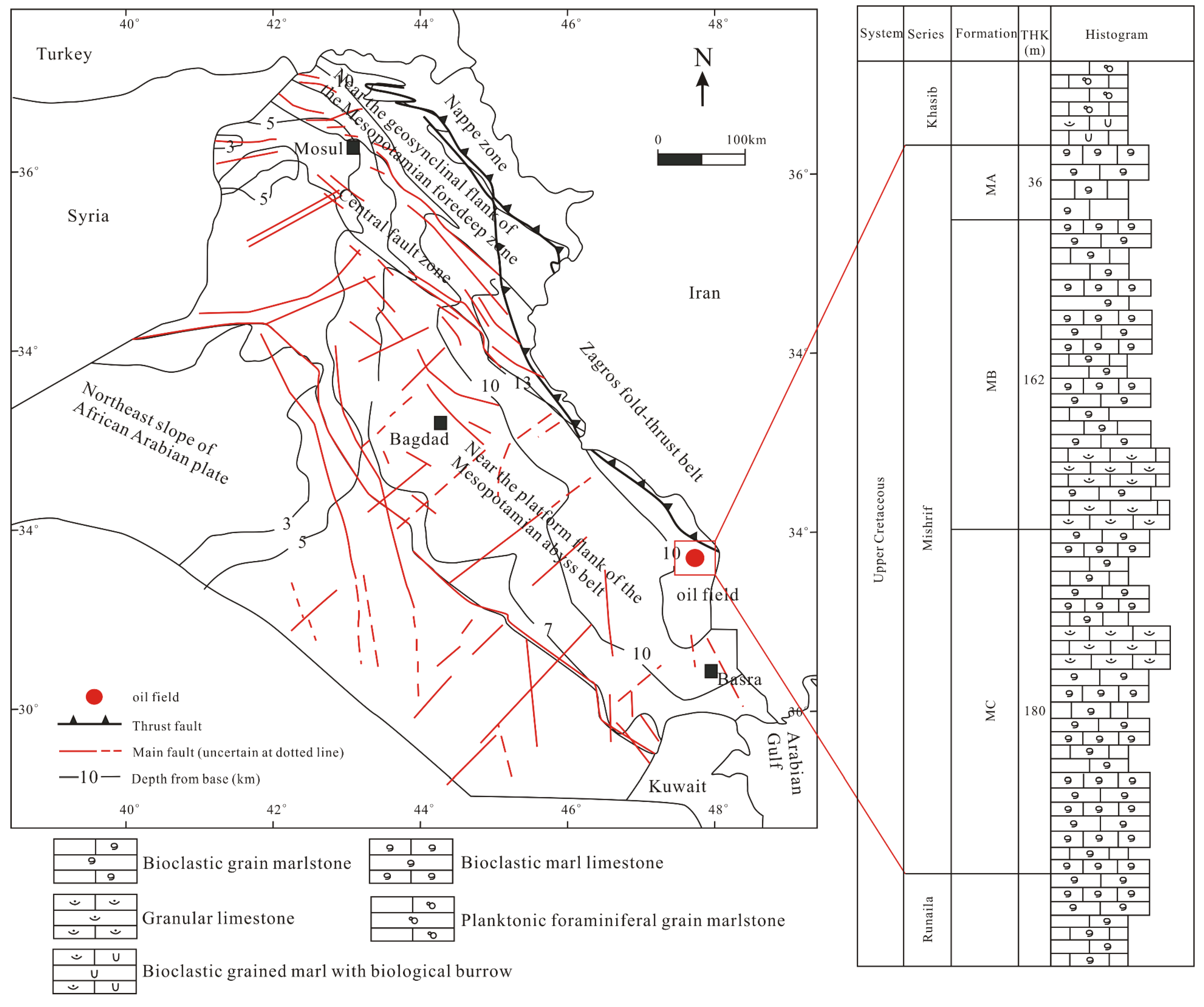
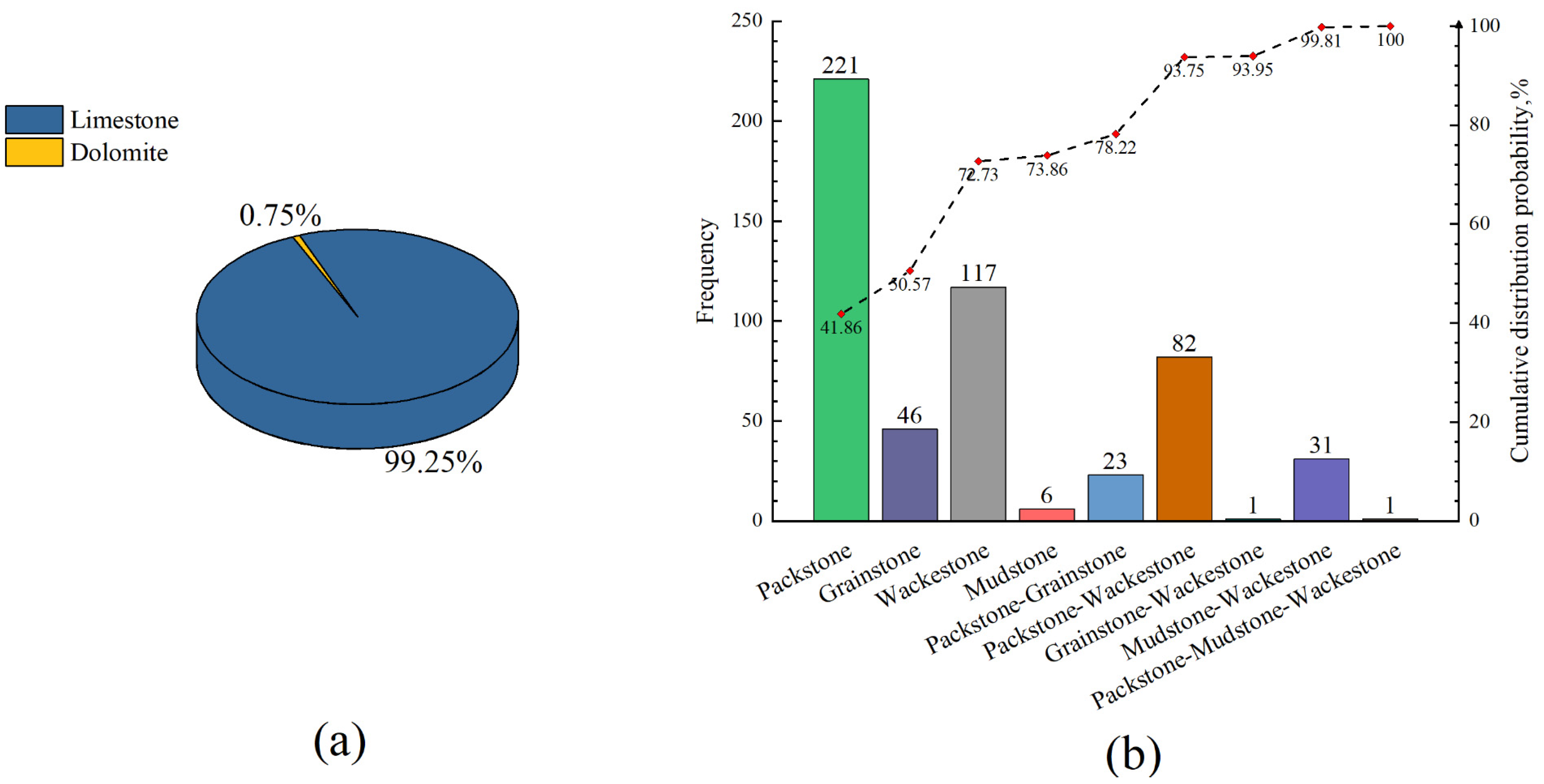
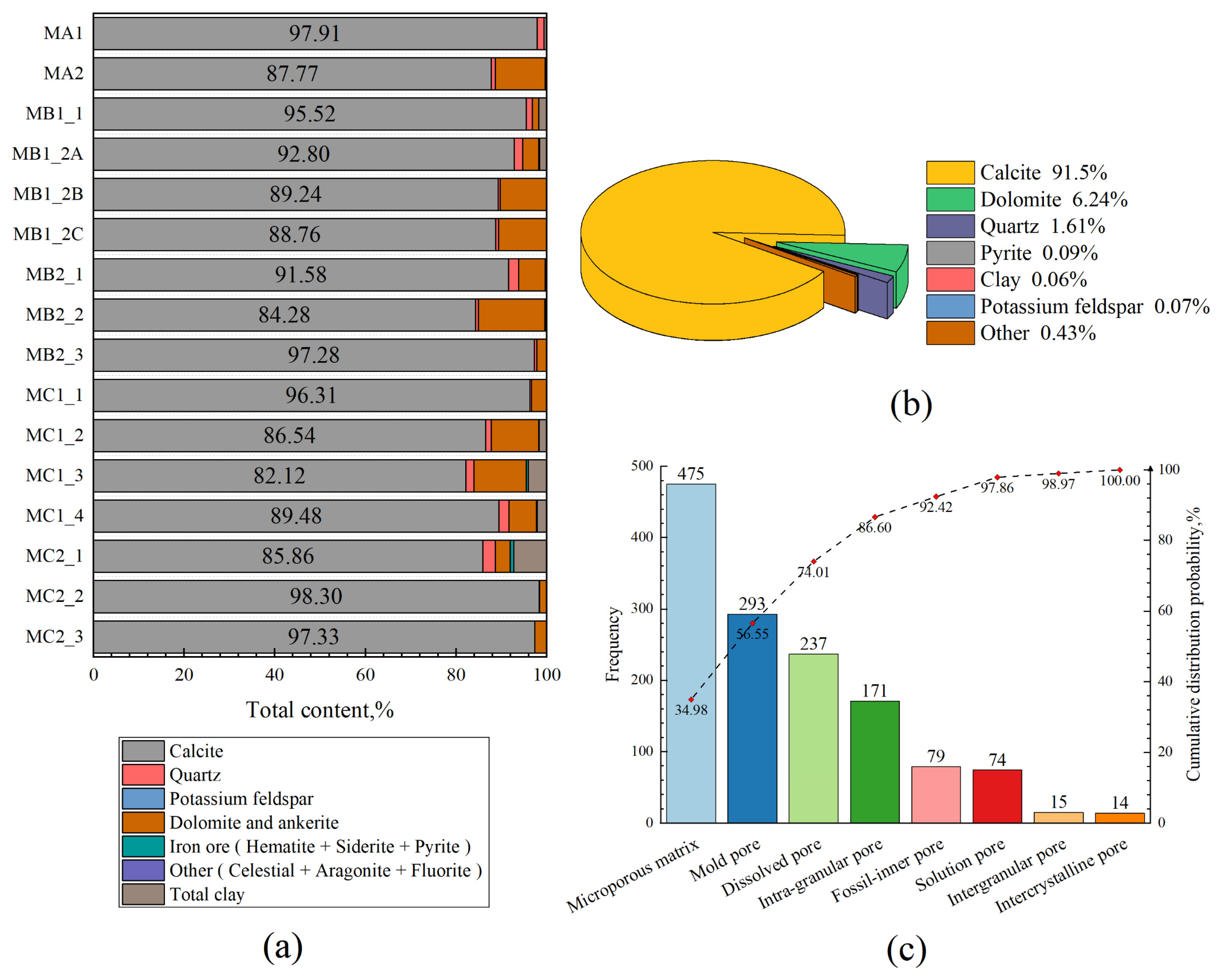
2. Geological Overview

The H oil field is located in the southeast of Iraq in the Middle East, south of Missan province, with a northwest–southeast trending back-slope structure (Figure 1) in the Mesopotamian fore-abyssal sub-basin. Tectonically, the M Formation group is in the southern part of the main Mesopotamian belt and the Euphrates sub-basin; it is the most thickly deposited, deeply buried, and tectonically stable tertiary unit in the Mesopotamian basin [4,29,30,31,32].

The thin section data corresponding to the target layer in the study area show that there are 528 blocks of limestone and 4 blocks of dolomite (Figure 2a); the M Formation is a pure limestone reservoir. According to Dunham’s classification criteria for limestones [33], the distribution of limestones in the target blocks includes packstones, grainstones, wackestones, and mudstones, with all types intermingled with one another. Packstone accounts for 41.86% of limestones, grainstone for 8.71%, wackestone for 22.16%, mudstone for 1.14%, packstone–grainstone for 4.36%, packstone–wackestone for 15.53%, grainstone–wackestone for 0.19%, mudstone–wackestone for 5.87%, and packstone–mudstone for 0.19%; the study area is mainly dominated by packstones and wackestones (Figure 2b).

For the lithological characteristics of the M formation, XRD (X-ray rock diffraction) analysis data were collected from five wells (Figure 3a); the mineral content statistics are shown in Figure 3b. The main mineral of the M formation is calcite, accounting for 91.5%; other minerals include dolomite (6.24%), quartz (1.61%), a small amount of pyrite (0.09%), and very few clay minerals accounting for about 0.06%. In addition, the percentages of various pore space types were determined based on the thin sections of core casts of the M-layer group in this block (Figure 3c). From Figure 3c, it can be seen that the pore space types in the study area are complex and diverse, mainly including microporous matrices, mold pores (connected or unconnected), dissolved pores, and intergranular pores. The area contains a certain number of fossil inner pores and solution pores and is interspersed with a very small number of intergranular pores and intercrystalline pores.

The reservoirs of the M Formation form multiple types of pores under different depositional environments [34], and the complex pore types also result in a complex pore structure and non-homogeneity in the study area.

3. Principle of the Method

3.1. Improved Archie Formula for Water Saturation

3.1.1. Traditional Archie Formula

The relationship between water saturation and formation variables (formation resistivity and formation water resistivity) is established by Archie’s formula [10]. Based on experiments on pure sandstone cores, the formation factor $F$ and the resistance increase coefficient $I$ are proposed as shown in Equations (1) and (2). The intersection of the formation factor and porosity is plotted in double logarithmic coordinates, and the relationship between $F$ and porosity is fitted by least squares regression with the slope of the straight line being the cementation index $m$ and the intercept being the cementation constant a, corresponding to the ratio of resistivity to brine resistivity for pure sandstone cores with different porosity containing brine. The intersection of the formation resistance increase coefficient and water saturation is plotted in double logarithmic coordinates, and the relationship is fitted by least squares regression. The slope of the straight line is the saturation index $n$, and the intercept of the straight line is the saturation constant b, which corresponds to the ratio between the resistivity and brine resistivity of pure sandstone cores with different water saturation. Combining Equations (1) and (2) yields the classical Archie model (Equation (3)). Equation (3) shows the numerical relationship between water saturation and the parameters of formation water resistivity, formation resistivity, porosity, cementation index, and saturation index [10].

$$F=\frac{a}{{\varphi }^m}=\frac{R_o}{R_w}$$

(1)

$$I=\frac{b}{S_w{}^n}=\frac{R_t}{R_o}$$

(2)

$$S_w=\sqrt[n]{\frac{a\times b\times R_w}{R_t\times {\varphi }^m}}$$

(3)

where $F$ is the formation factor, dimensionless; $a$ is the cementation constant, dimensionless; $m$ is the cementation index, dimensionless; $\varphi$ is the porosity, fraction; $R_o$ is the resistivity of the formation saturated with brine, Ohm.m; $R_w$ is the resistivity of formation water, Ohm.m; $I$ is the resistance increase coefficient, dimensionless; $b$ is the saturation constant, dimensionless; $S_w$ is the water saturation, fraction; and $R_t$ is the resistivity of formation, Ohm.m.

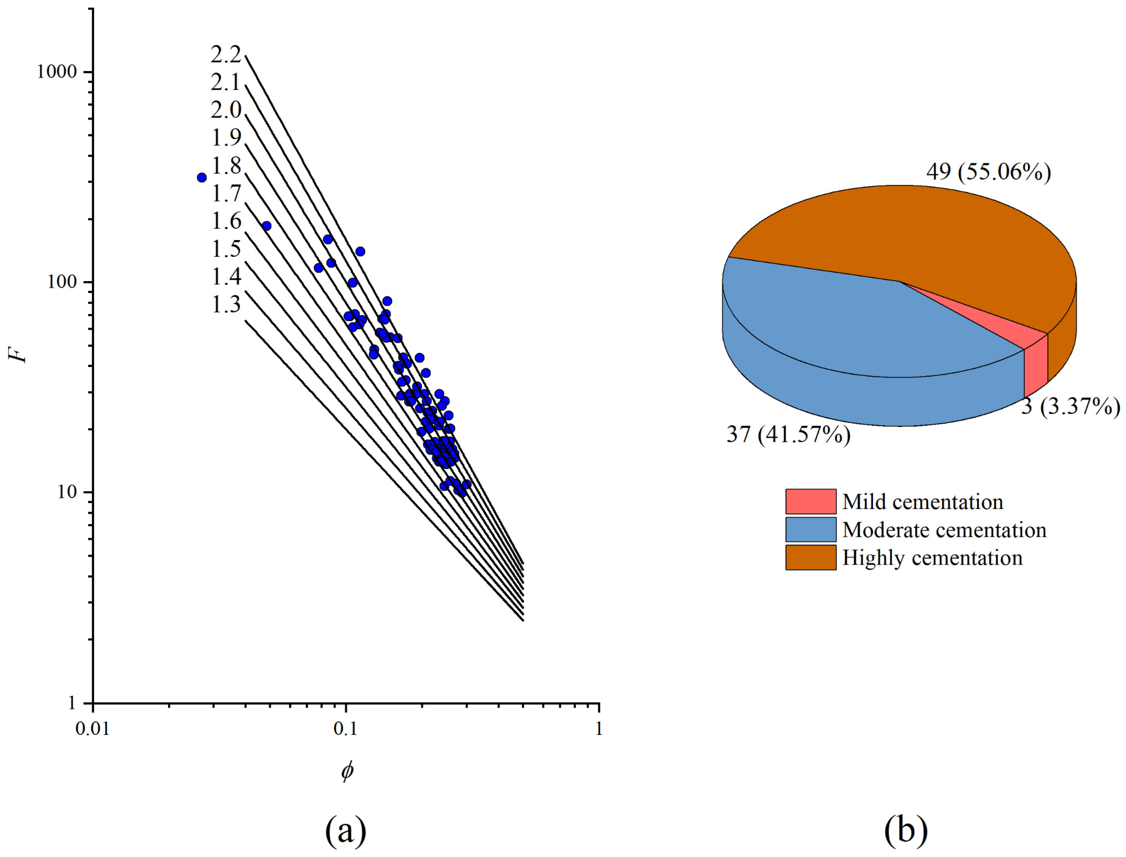
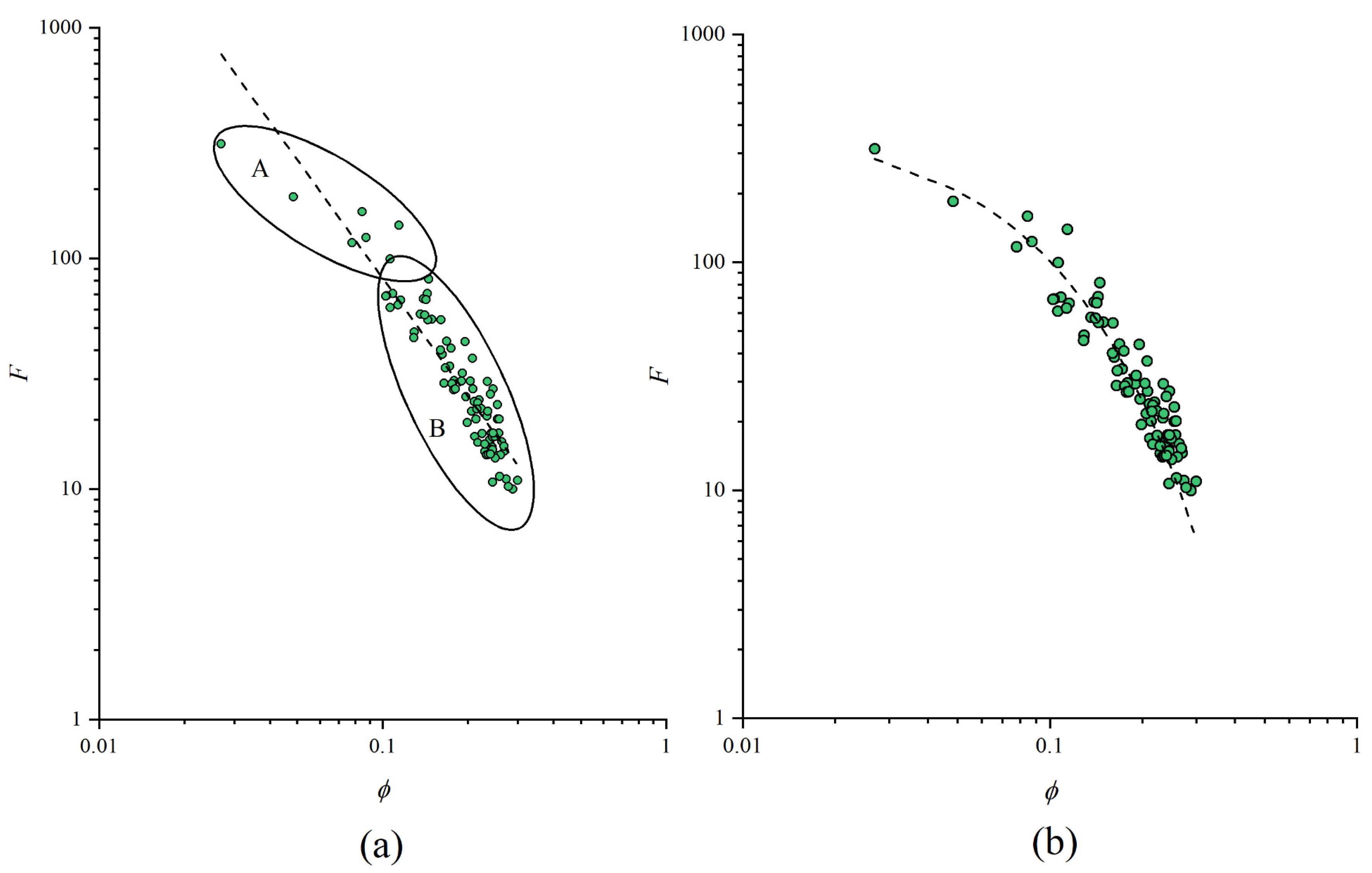
3.1.2. Variation of the Cementation Index

In Archie’s formula (Equation (3)), $m$ is taken as a constant, which is based on the assumption that rock samples have similar pore geometry but with different degrees of porosity and diagenesis. The cementation index in Archie’s formula is calculated as in Equation (4) where a is taken as 1. The degree of cementation of rocks is classified as no cementation, slight cementation, mild cementation, moderate cementation, and high cementation according to the magnitude of $m$ values [35]. The range of $m$ values of 89 cores in the study block was determined (Figure 4a), and it can be found that the degree of cementation in the M-layer group is mainly high and moderate cementation (Figure 4b), which reflects the complexity of carbonate rocks in the study area.

$$m=-\frac{Lo{g}_{10}(F)}{Lo{g}_{10}(\varphi )}$$

(4)

That is, taking different $m$ values for different strata can theoretically reflect the actual cementation of the strata more accurately, especially in carbonates with diverse pore structures.

Similarly, Figure 5a gives the relationship between formation factors and reservoir porosity for each core with porosity distributed between 3% and 30% and formation factors distributed in the interval of 9–320. Using the distribution law of formation factors and porosity, the relationship can be divided into two zones, zone A and zone B. Among them, the relationship between formation factors and porosity in zone B is in accordance with Archie’s law, and the trend line intersects near the point (1,1). However, the formation factors and porosity in zone A violate Archie’s law and demonstrate “non-Archie” phenomenon according to the fitting results (Equation (5) in

Table 1. The fitting relationship results and goodness of fit of the cementation index, formation factor, and resistance increase coefficient.

Formula	Number of Samples	${\mathit{R}}^2$	Formula No.
$F=\frac{1.62}{{\varphi }^{1.70}}$	89	0.80	(5)
$m=71.91{\varphi }^3-48.48{\varphi }^2+10.13\varphi +1.40$	89	0.14	(6)
$F=\frac{415.36}{e^{14.13\varphi }}$	89	0.92	(7)
$I=\frac{1.04}{S_w{}^{1.89}}$	291	0.95	(8)

); the parameters in Equation (1) are taken as a = 1.62 and $m$ = 1.70. At the same time, the regression of the cementation index and porosity (Equation (6) in Table 1) shows the fit is low, which also indicates that regardless of the constant value of $m$, a direct relationship between $m$ and porosity is not appropriate. This is due to the fact that although Archie’s formula is applicable to pure sandstone formations with low mud content, and although the carbonate reservoir in the study area has low mud content, the actual reservoir has diverse and complex pore types with strong non-homogeneity, which is the reason for the “non-Archie” phenomenon in the samples at low values of porosity in the petrophysical experiments. Although the basic morphology can be shown, the inaccuracy of a and $m$ values will affect the applicability of the model. In this paper, by changing the shape of Archie’s formula, avoiding the calculation of $m$ value, and determining the water saturation based on the rendezvous relationship between formation factors and porosity, the exponential function relationship between formation factors and porosity is reconstructed (Figure 5b), and a better correlation is achieved (Equation (7) in Table 1) with the goodness of fit reaching 0.92.

The classical Archie formula can be written as

$$S_w=\sqrt[n]{\frac{b\times F\times R_w}{R_t}}$$

(9)

Using the form of Equation (7), one can rewrite Archie’s formula as

$$S_w=\sqrt[n]{\frac{c_1\times b\times R_w}{e^{c_2\times \phi }{R}_t}}$$

(10)

According to Equation (10), the problem of selecting the cementation index $m$ can be avoided.

The lithology of the M formation is pure, and the mud content is low. Theoretically, Archie’s formula is practical, but the direct use of Archie’s formula to obtain the rock-electric parameters reveals that the cementation index $m$ does not take a constant value. This paper aims to solve this problem by means of fitting with a method similar to that for fitting the cementation index using porosity; however, the fitting effect is found to be poor when using Equation (6). Therefore, the most suitable fitting formula in a mathematical sense is adopted in this paper, and the best result is obtained analytically when Equation (7) is used; thus, Archie’s formula is improved based on this equation. The applicability of the formula needs further explanation as follows: For the same geological background, taking the reservoir containing the same M formation in the neighboring country of Y as an example, it may be equally applicable when the geological background does not change much; however, when the geological background changes and the rock pore type and mud content change greatly, the analysis needs to be carried out according to the actual experimental parameters.

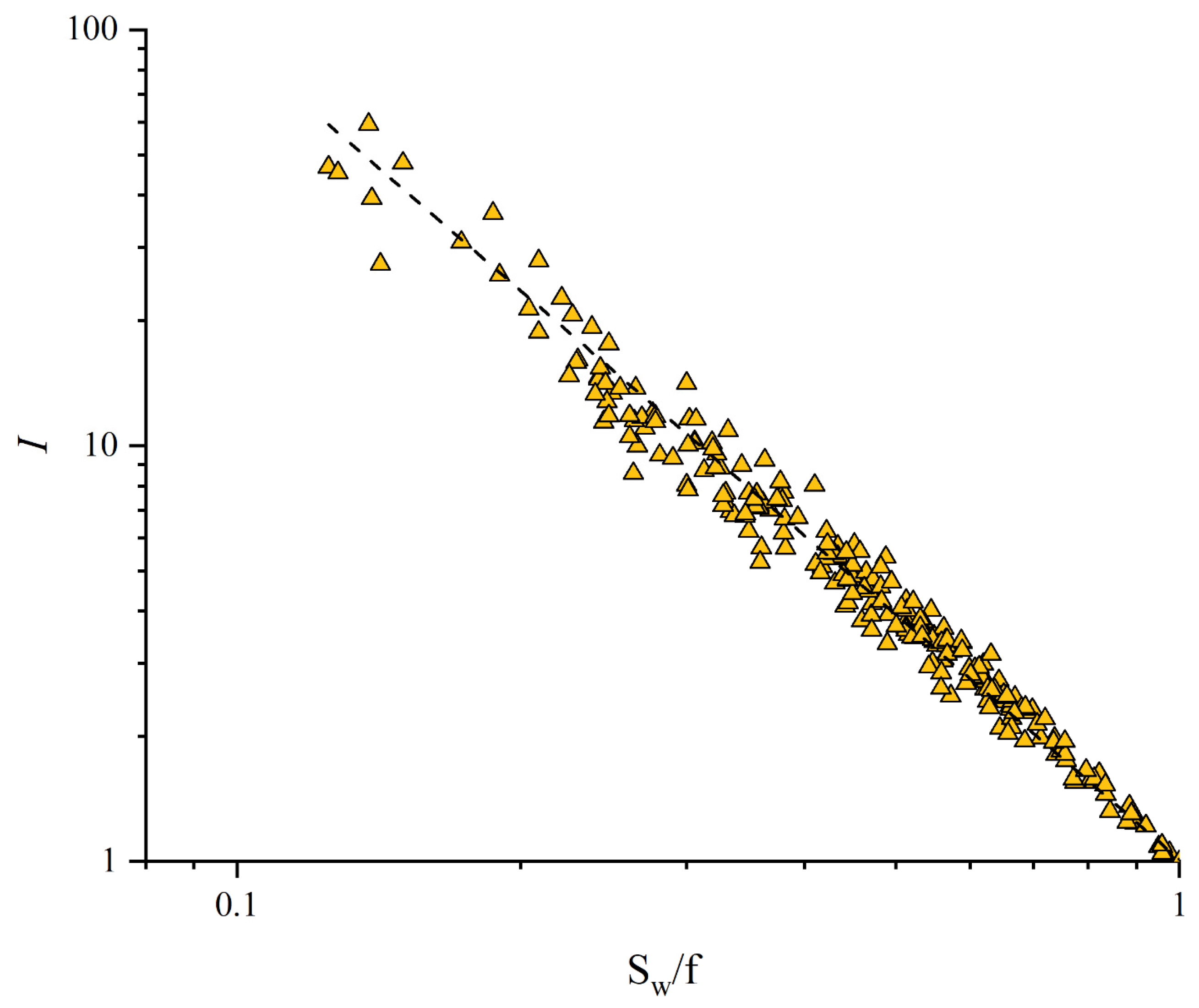
3.1.3. Study of the Relationship between Resistance Increase Coefficient and Water Saturation

After determining the new formula for water saturation, it remains necessary to determine b and the saturation index $n$ in the formula. Figure 6 shows a plot of 291 sets of resistance increase coefficients and the water saturation rendezvous for 49 cores of the M formation. From Figure 6, it can be seen that $I$ has a good relationship with $S_w$ (Equation (8) in Table 1), and the goodness of fit is 0.95.

The saturation index is affected by the wettability, pore structure, temperature, pressure, and mineralization of the formation water. The more hydrophilic the rock, the higher the temperature, or the higher the mineralization of the formation water, the lower the value of $n$. The more oleophilic the rock, the more complex the conductive pathway, or the higher the pressure, the higher the value of $n$. In laboratory conditions, temperature, pressure, and formation water mineralization are at or near a constant, and their effects are negligible [36]. The wettability of the rocks is a key factor affecting the saturation index, and the rock wettability of the M formation has similar wettability through the 49 cores collected, distributed between layers MA1 and MC1_1. In summary, the final saturation index $n$ is 1.89, and the value of b is taken as 1.04.

From the above analysis of the rock-electric experimental data, the table of calculated parameters of water saturation for the M formation group in the H field in the Middle East is shown in

Table 2. Parameters of water saturation calculation formula of carbonate reservoir in the study area.

Parameter	${\mathit{c}}_1$	${\mathit{c}}_2$	b	$\mathit{n}$
	415.36	14.13	1.04	1.89

.

3.2. Fluid Property Identification Method Based on Total Differential Method

In this paper, based on the actual situation of the M-layer group, the problem of taking the values of a and $m$ is avoided and improved, as shown in Equation (10). Similar to Equation (3), the equation assumes that the lithology coefficient $b$, $n$, and formation water resistivity $R_w$ change with depth, while their values remain constant within the same depth, and the main factors in the equation are porosity and water saturation. In the identification of fluid properties of oil and water formations, resistivity is commonly used to make judgments; thus, Equation (10) can be rewritten as

$$R_t=\frac{c_1\times b\times R_w}{e^{c_2\times \varphi }\times S_w{}^n}$$

(11)

Based on Equation (11), combined with the traditional differential method [37], the differential treatment of porosity and water saturation can be expressed using two new formulas as follows:

$$DRTP=\frac{\partial R_t}{\partial \varphi }=\frac{-c_1\times c_2\times b\times R_w}{e^{c_2\times \varphi }\times S_w{}^n}$$

(12)

$$DRTS=\frac{\partial R_t}{\partial S_w}=\frac{-n\times c_1\times b\times R_w}{e^{c_2\times \varphi }\times S_w{}^{(n+1)}}$$

(13)

Then, two sets of discriminatory criteria can be obtained according to the above two formulas, i.e., when the water saturation is equal to the irreducible water saturation ($S_w=S_{wir}$), the two sets of values obtained are termed the oil layer discriminant values (Equations (14) and (15)):

$$OLIP={\frac{\partial R_t}{\partial \varphi }|}_{S_w=S_{wir}}=\frac{-c_1\times c_2\times b\times R_w}{e^{c_2\times \varphi }\times S_{wi}{}^n}$$

(14)

$$OLIS={\frac{\partial R_t}{\partial S_w}|}_{S_w=S_{wir}}=\frac{-n\times c_1\times b\times R_w}{e^{c_2\times \varphi }\times S_{wi}{}^{(n+1)}}$$

(15)

Equation (14) is the formula for the oil layer discriminant value after differentiation of resistivity on porosity, which is referred to as $OLIP$ in this paper, and Equation (15) is the formula for the oil layer discriminant value after differentiation of resistivity on water content saturation, which is referred to as $OLIS$ in this paper.

Similarly, when the water saturation is equal to 1 ($S_w=1$), 2 sets of values can be obtained, which are termed the water layer discriminant values (Equations (16) and (17)):

$$WLIP={\frac{\partial R_t}{\partial \varphi }|}_{S_w=1}=\frac{-c_1\times c_2\times b\times R_w}{e^{c_2\times \varphi }}$$

(16)

$$WLIS={\frac{\partial R_t}{\partial S_w}|}_{S_w=1}=\frac{-n\times c_1\times b\times R_w}{e^{c_2\times \varphi }}$$

(17)

Equation (16) is the formula for the water layer discriminant value after differentiation of resistivity to porosity, which is referred to as $WLIP$ in this paper, and Equation (17) is the formula for the water layer discriminant value after differentiation of resistivity to water-bearing saturation, which is referred to as $WLIS$ in this paper.

Correspondingly, in terms of porosity: (1) when the calculated value is equal to the oil layer discriminant value ($DRTP=OLIP$), the fluid nature can be judged as the oil layer; (2) when the calculated value is equal to the water layer discriminant value ($DRTP=WLIP$), the fluid nature can be judged as the water layer; and (3) when the calculated value is between the oil layer discriminant value and the water layer discriminant value ($WLIP<DRTP<OLIP$), the fluid nature can be judged as oil–water layer.

Similarly, in terms of water saturation: (1) when the calculated value is equal to the oil layer discriminant value ($DRTS=OLIS$), the fluid nature can be judged as the oil layer; (2) when the calculated value is equal to the water layer discriminant value ($DRTS=WLIS$), the fluid nature can be judged as the water layer; and (3) when the calculated value is between the oil layer discriminant value and the water layer discriminant value ($WLIS<DRTS<OLIS$), the fluid nature can be judged as the oil–water layer.

This method mentioned above constructs two sets of fluid property identification processes based on the improved Archie formula, which are based on porosity and water saturation. However, in practice, considering the non-homogeneity of the reservoir, the identification results of the two sets of processes may be inconsistent, which in turn limits the practical application of this method. Therefore, this paper optimizes this method by differentiating both porosity and water-bearing saturation based on Equation (11), obtaining the following:

$$RTPW=\frac{{\partial }^2{R}_t}{\partial \varphi \partial S_w}=\frac{c_1\times c_2\times n\times b\times R_w}{e^{c_2\times \varphi }\times S_w{}^{(n+1)}}$$

(18)

The corresponding oil layer discriminant value ($RTSO$) and water layer discriminant value ($RTSW$) are given in Equations (19) and (20):

$$RTSO={\frac{{\partial }^2{R}_t}{\partial \varphi \partial S_w}|}_{S_w=S_{wir}}=\frac{c_1\times c_2\times n\times b\times R_w}{e^{c_2\times \varphi }\times S_{wi}{}^{(n+1)}}$$

(19)

$$RTSW={\frac{{\partial }^2{R}_t}{\partial \varphi \partial S_w}|}_{S_w=1}=\frac{c_1\times c_2\times n\times b\times R_w}{e^{c_2\times \varphi }}$$

(20)

The above equations correspond to the parameters specified in Table 2.

In summary, this paper improves Archie’s formula based on the M-layer group and proposes a new set of fluid property identification methods based on the improved formula, applying this method to the M-layer group. It should be noted that the saturation of irreducible water as one of the key parameters for judging fluid properties is calculated by applying machine learning methods in this paper (see Section 4 for further detail).

4. Results and Discussion

4.1. Saturation Prediction Results

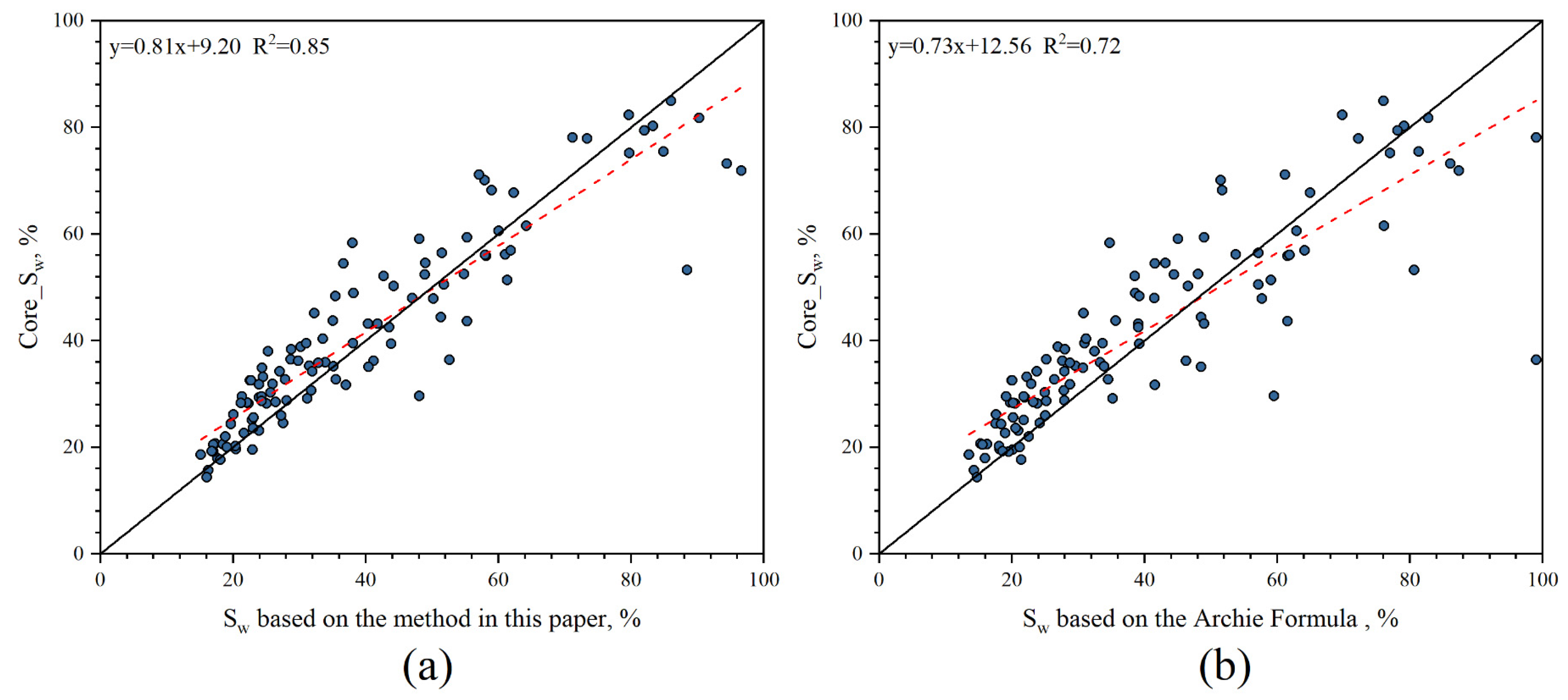
4.1.1. Water Saturation Prediction Results

The new formula for water saturation using the values of each parameter is given in Section 3.1. The determination of the formation water resistivity was performed using the formation water analysis data. A total of 5 groups of formation water analysis data were collected, and the total mineralization of formation water was in the range of 181,230–212,360 mg/L. The final formation water resistivity of 0.02 Ohm.m was obtained by calculating the average value of formation water resistivity for the 5 groups.

The water saturation was calculated based on the above parameter values, and the improved method of this paper was implemented and compared with the conventional Archie formula model. It should be noted that the core water saturation data are limited, and corrections are required for the comparison [38,39]. Figure 7 and Figure 8 show the results of the method of this paper and the traditional Archie formula in the calculation of water saturation, respectively. Figure 7a shows the comparison between the calculated results of this paper’s method and the core data, and Figure 7b shows the comparison between the calculated results of the traditional Archie formula and the core data, including the fitting formula and the goodness of fit of the calculated results and the core results. Figure 8 further clarifies the error distribution of the two methods. Figure 7a shows the effect of the method in this paper, and the calculated results are compared with the core water saturation. The goodness of fit of the results of this method with the core data is 0.85, and the relative error ranges from 0.18 to 66.01% with an average relative error of 14%. Meanwhile, when the water saturation is calculated based on the conventional Archie formula and compared with the core data, the goodness of fit is 0.72, and the relative error ranges from 0.59 to 177.97% with an average relative error of 21%. It should be noted that when the calculated error of water saturation exceeds 100%, the default upper limit is 99% in order to be shown in the figure, and there are 2 points immediately adjacent to the right y-axis in Figure 7b. By analyzing Figure 8, the error of water saturation calculated by the improved method is generally low when compared to the traditional Archie formula with no extreme error value. When the porosity is very small, the traditional Archie formula is not suitable for the value of a and m in the A area (Figure 5a), which results in the error of water saturation as calculated by the traditional Archie formula too large, and the relative error exceeds 100%. The improved method can effectively reduce this kind of evaluation error, resulting in the maximum relative error of this method being significantly smaller than that of the traditional method. For the data with porosity above 8%, the error of water saturation predicted by the improved Archie model is 9.86%, and the error of water saturation predicted by the traditional Archie model is 15.98%. When comparing the core data, the method in this paper has stronger applicability without increasing the computational cost, especially in the face of low porosity reservoirs with better application effect.

4.1.2. Calculation of Irreducible Water Saturation

Among the fluid property identification methods proposed in this paper, the irreducible water saturation is one of the key aspects. In this paper, we use a mature machine learning method to construct the irreducible water saturation evaluation model [40,41,42]. The core irreducible water saturation was extracted using mercury injection capillary pressure (MICP) data; then, the irreducible water saturation prediction model was trained using the conventional geophysical logging data combined with the machine learning method and tested using the irreducible water saturation dataset, which was not involved in the model construction. Machine learning methods have been abundantly used in evaluating reservoir parameters with good application results. This paper uses the random forest method, which is not affected by weight settings and does not have to consider the effect of normalization on the data [43]; it was implemented using TECHLOG software. Figure 9a shows the back-judgment results of the irreducible water saturation prediction model, and Figure 9b shows the actual application effect of the test set. The analysis shows that the constructed irreducible water saturation prediction model can be effectively applied to the test data, and the goodness of fit of the training and test sets is similar. The effectiveness of this model is thus demonstrated.

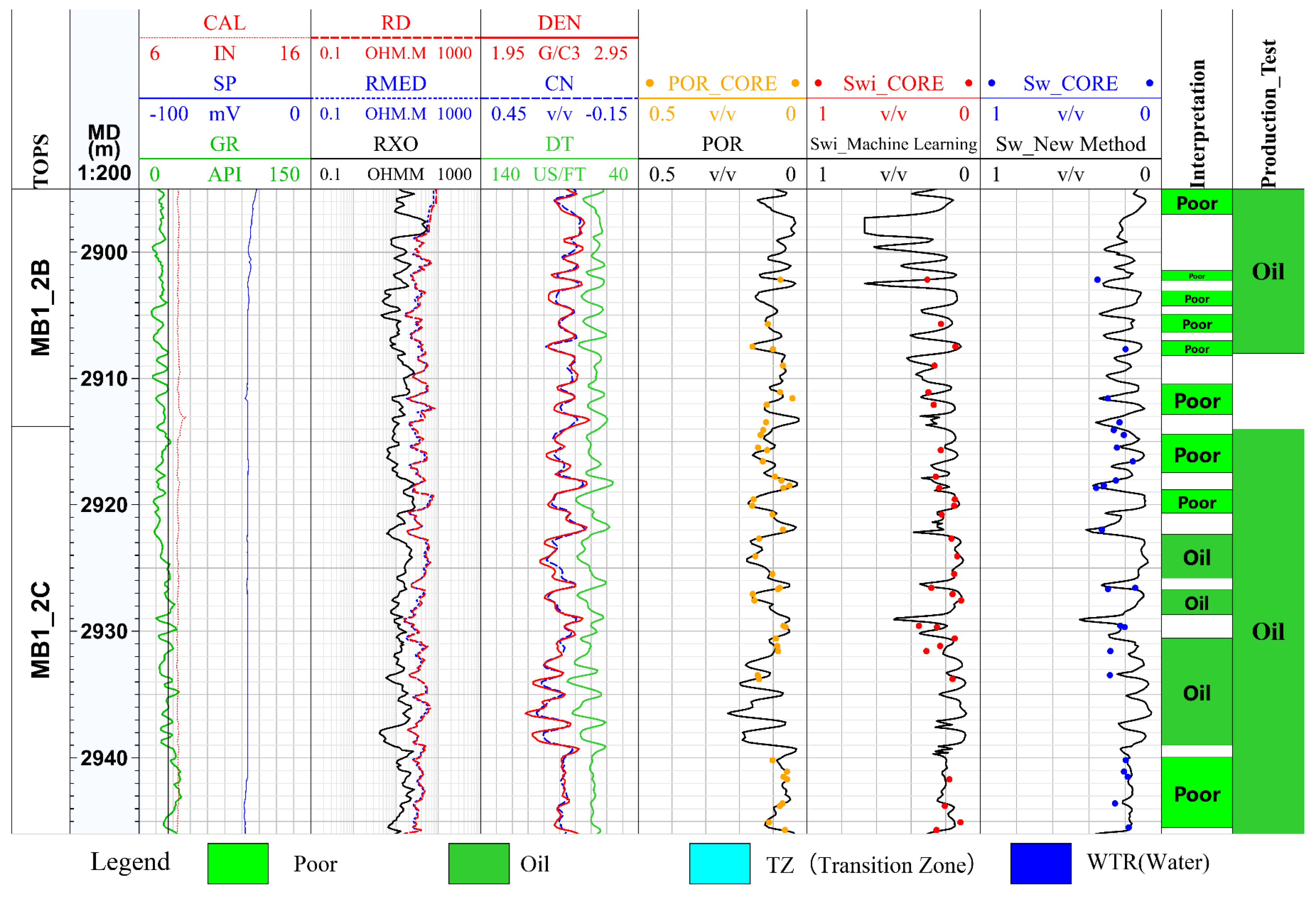
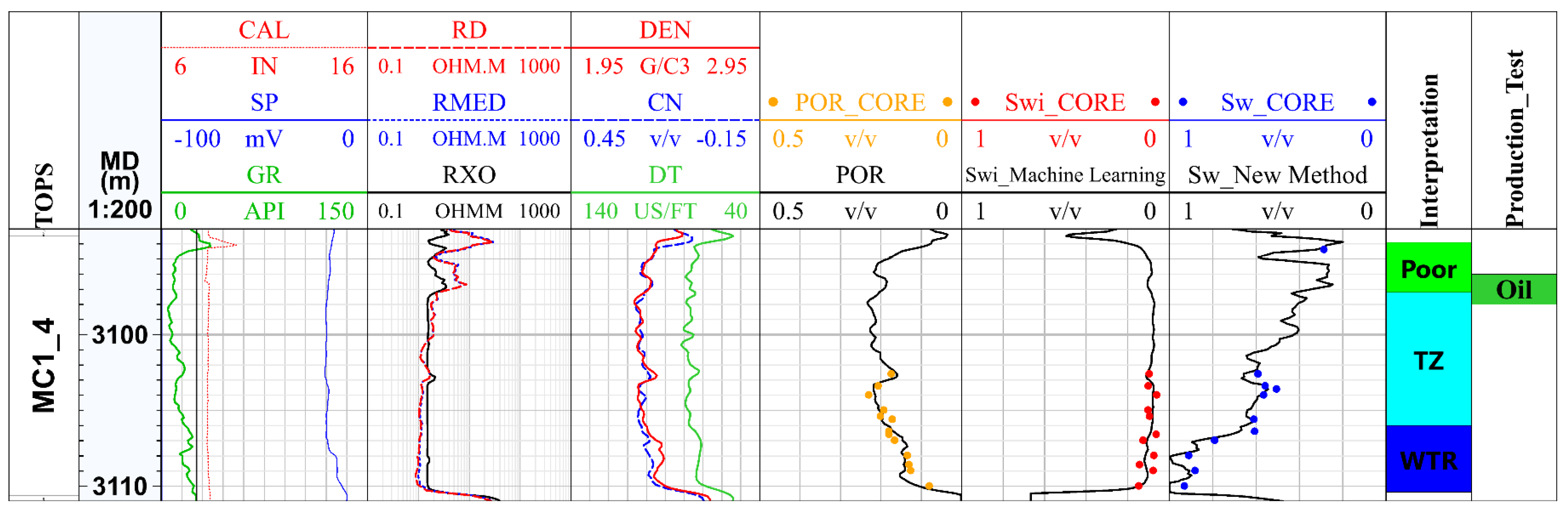
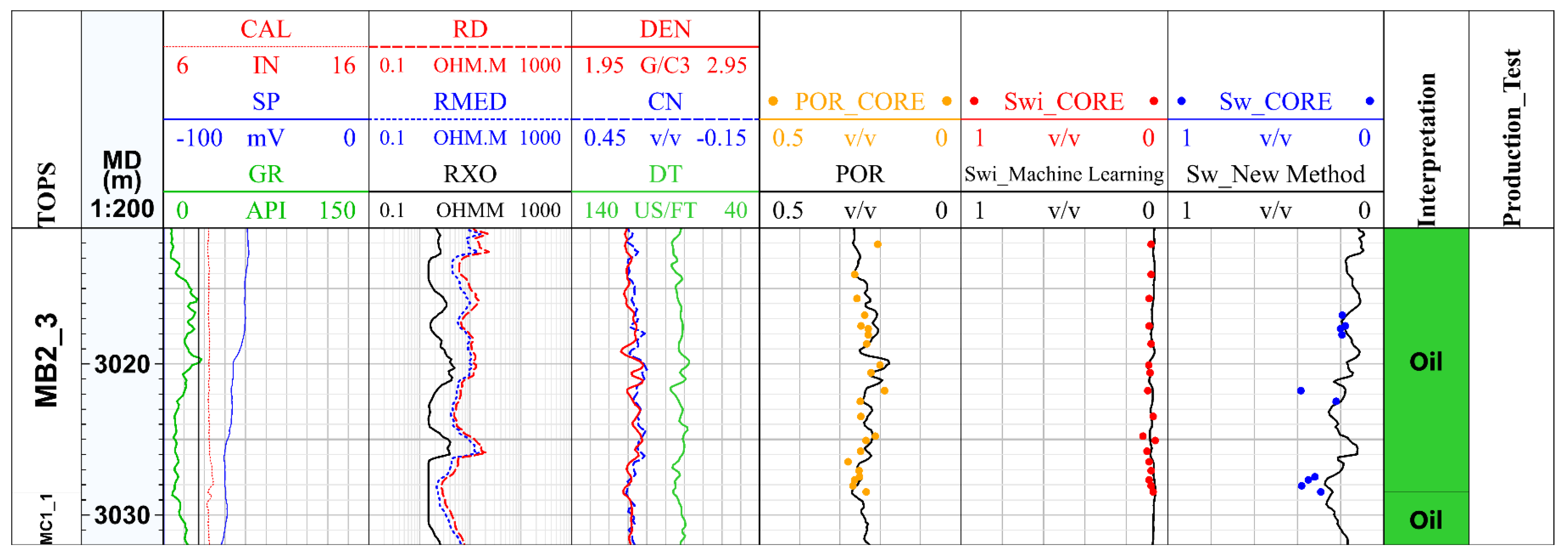
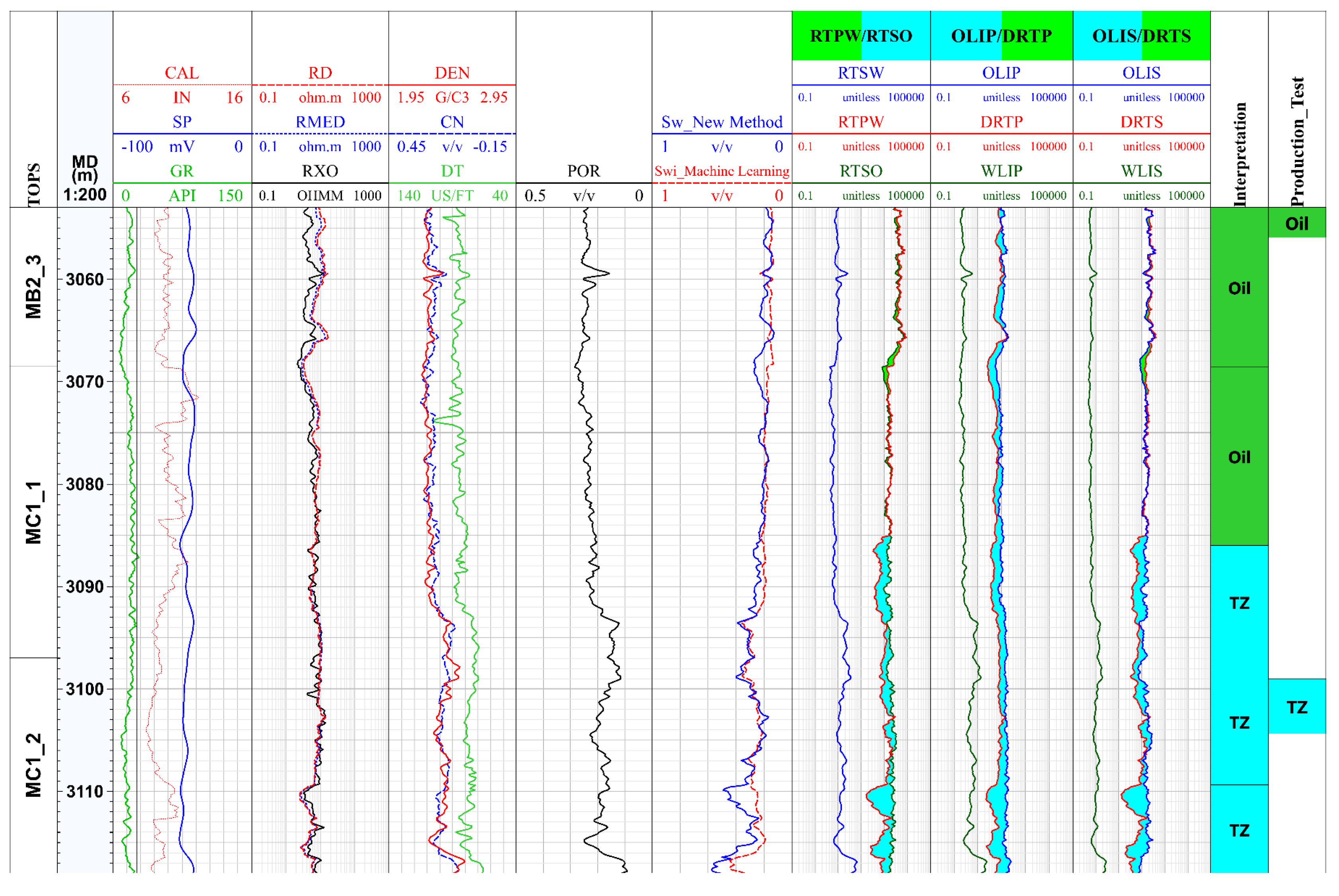
4.1.3. Saturation Prediction Example

The actual logging data are used as an example to show the effect of water saturation evaluation. Figure 10 and Figure 11 show the application of the core section for two wells. The first track is the formation channel, which gives the specific location of the M layer to which the section belongs; the second track is the depth channel, which gives the depth curve; the third track is the lithology curve channel, which contains the well diameter logging curve, natural potential logging curve, and natural gamma logging curve; the fourth track is the resistivity channel, which contains three resistivity curves with different detection depths from deep to shallow, namely, deep lateral resistivity log (RD), shallow lateral resistivity log (RMED), and flushed-zone resistivity log (RXO) series curves; the fifth track is the porosity curve channel, which includes the density logging curve, neutron logging curve, and acoustic time-difference logging curve; the sixth track is the porosity calculation result, which includes the porosity curve calculated by the neutron density rendezvous method and core porosity; the seventh track is the irreducible water saturation calculation result, which includes the irreducible water saturation curve, calculated based on the geophysical logging curve and core irreducible water saturation; the eighth track is the calculation result of water content saturation, including the water content saturation curve and core water content saturation as calculated by the method of this paper; the ninth channel is the interpretation conclusion channel, containing the interpretation conclusion of each reservoir; and the tenth channel is the oil test conclusion channel, including the industrial production judgment and test conclusion. Figure 10 shows the MB section of well A. By analyzing the seventh and eighth sections, the predicted results of the irreducible water saturation are compared with the core data. The prediction results of the irreducible water saturation of the well are in good agreement with the core data, which shows the reliability of the prediction of the irreducible water saturation. Meanwhile, the calculated water saturation results also maintain a high agreement with the core results. The reservoirs shown in well A are all oil layers or poor oil layers, and the calculated water saturation curves are consistent with the irreducible water saturation curves at the reservoirs both in terms of curve trends and values, which also demonstrates the effectiveness of the method in this paper. In addition, Figure 11 shows the MC section of well B, which contains different fluid properties during the spreading period. The calculated water saturation increases at the oil–water layer (transition zone), but the irreducible water saturation does not increase. The analysis of the actual well data shows the effectiveness of the method in this paper.

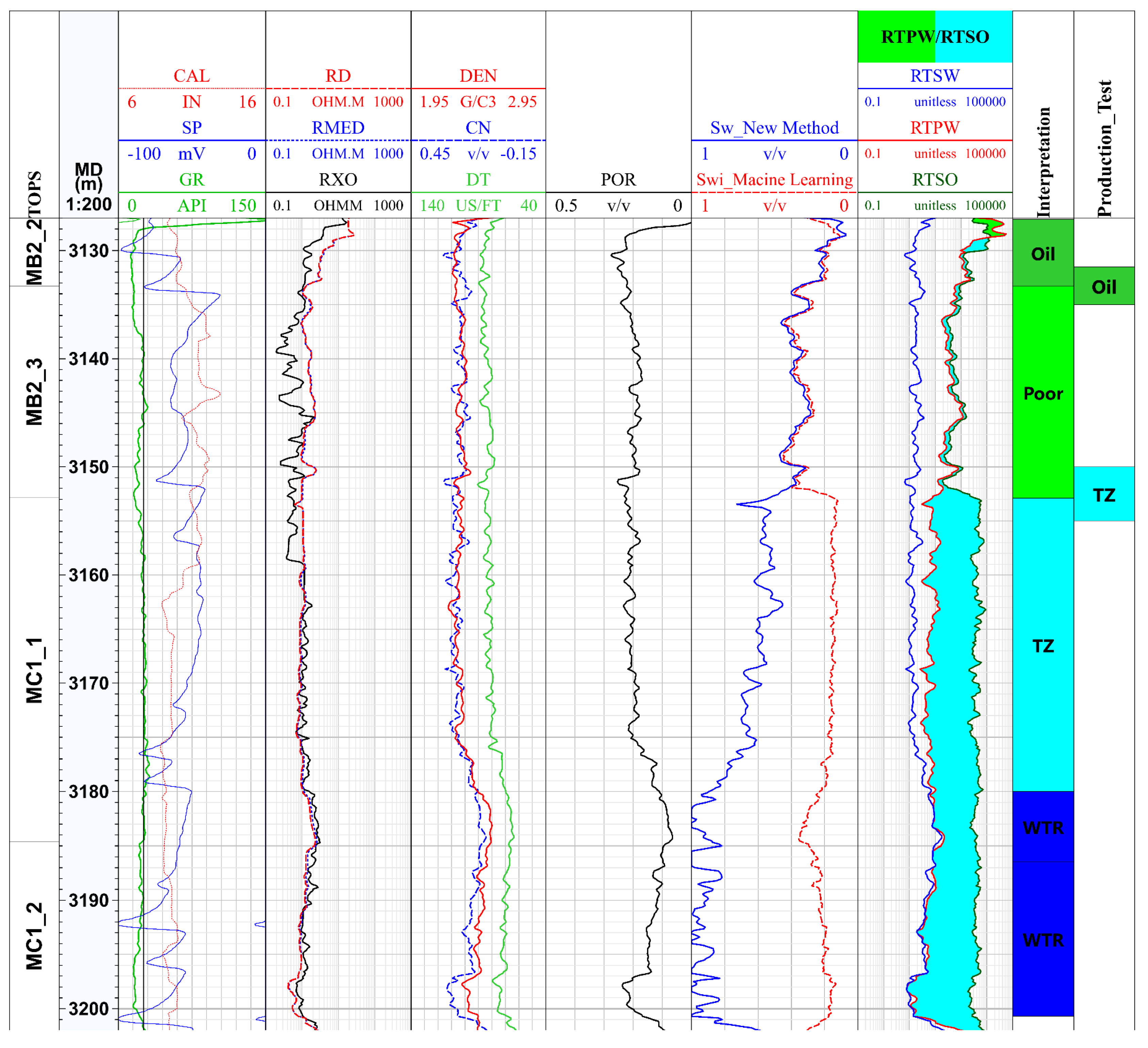
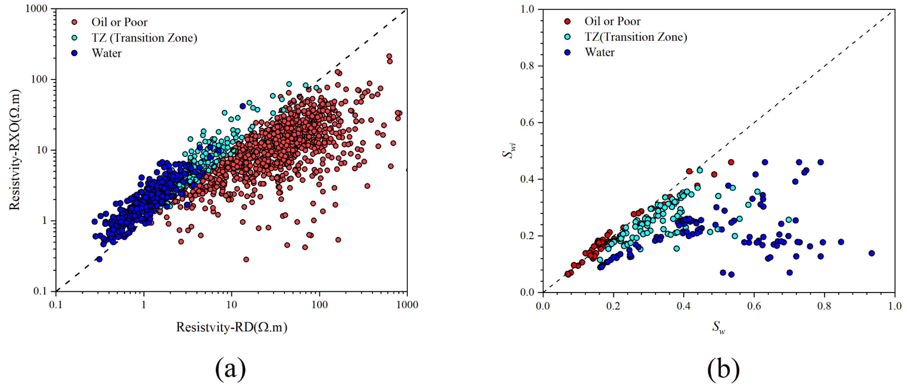
4.2. Results of the Application of the Total Differentiation Method

After calculating the water saturation and irreducible water saturation, the fluid properties can be identified using the total differential method, which is shown for an actual well. Figure 12 contains ten tracks, and compared to Figure 10, the seventh and eighth tracks differ in the figure. The eighth track shows the results of the total differential method, including the calculated curve $RTPW$, the oil layer discriminant line $RTSO$, and the water layer discriminant line $RTSW$, and is filled in green when the calculated curve exceeds the oil layer discriminant line and in blue when the curve is between the oil layer discriminant line and the water layer discriminant line. Taking the MB and MC sections of well C as an example, the results of water saturation and irreducible water saturation calculations are consistent at the differential oil layer of MB2_3. In the corresponding total differential method, the calculated line is parallel to the oil layer discriminant line, and numerically the calculated line is slightly lower than the oil layer discriminant line. In the transition zone where oil and water are in the same layer, the calculated line rapidly approaches the water layer discriminant line, and the two overlap at the water layer. Combining the oil test conclusion with the test result, the oil formation section matches, and the water production rate of the test section is 17%, which matches with the judgment result of the total differential method. Therefore, the fluid properties of the reservoir can be accurately identified using the total differential method, and the transition zone can be accurately delineated in the same oil–water system, giving the exact location of the oil-down-to (ODT) and the water-up-to (WUT) levels.

The calculation results of the total differential method were validated for the M layer group in the study area, and the validation data were obtained from the production conclusions and drill stem test (DST) conclusions. A total of 354 groups of layer segments were collected from 97 wells. Corresponding to the production or testing conclusions, there are 209 groups of oil layers, 98 transition zones (oil–water layers), and 47 water layers. Using the total differential method to judge these layer groups, the accuracy rate reached 89.55%. The corresponding confusion matrices are given in

Table 3. The confusion matrix of the fluid property discrimination results of the target block M layer using the total differential method.

Accuracy Rate (89.55%)	Prediction Results of the Total Differential Method
Test Results	Oil or Poor	Transition Zone	Water
Oil or Poor	196 (93.78%)	13 (6.22%)	0 (0.00%)
Transition zone	11 (11.22%)	84 (85.72%)	3 (3.06%)
Water	0 (0.00%)	5 (10.64%)	42 (89.36%)

. By analyzing the confusion matrix, all three fluid properties were effectively identified, and a small number of reservoirs in oil and water layers were identified as transition zones with oil and water in the same layer. Fourteen groups of transition zones were misidentified as oil or water layers with such errors mainly due to the discrimination errors between ODT and WUT. Geophysical logging data is acquired at the junction and at the top or bottom of the reservoir. Combined with the confusion matrix, it is found that the total differential method is effective for the identification of fluid properties.

The total differential method, as an effective fluid property identification method, can effectively identify the reservoir fluid properties. Two profiles in the H field are shown in Figure 13 with the NSEW1-1 well as the junction well, which is oriented east–west and south–north, respectively. The wells on these two lines are interpreted, and the fluid properties are discriminated using the total differential method and plotted as profiles in Figure 14. The two profiles in Figure 14 are made from a total of 17 wells. The first contains the GR curve and DEN curve; the second is the depth curve, giving the true vertical depth (TVD) and true vertical depth subsea (TVDSS); the third contains the formation information and interpretation conclusion; the fourth is the interpretation conclusion; and the fifth is the test result. Figure 14a is the south–north oriented oil–water section, showing the fluid property identification results of MA1-MC1-2 in the M Formation; for the south–north oriented section, the ODT and WUT are shallow in the south and deep in the north, and the transition zone is relatively undulating. Figure 14b is the east–west oriented oil–water section; the ODT and WUT are shallow in the east and deep in the west, and the thickness of the transition zone is relatively stable. The ODT depths of the two profiles vary from −3071~−3033 m, and the WUT depths can reach up to −3048.7 m.

4.3. Discussion

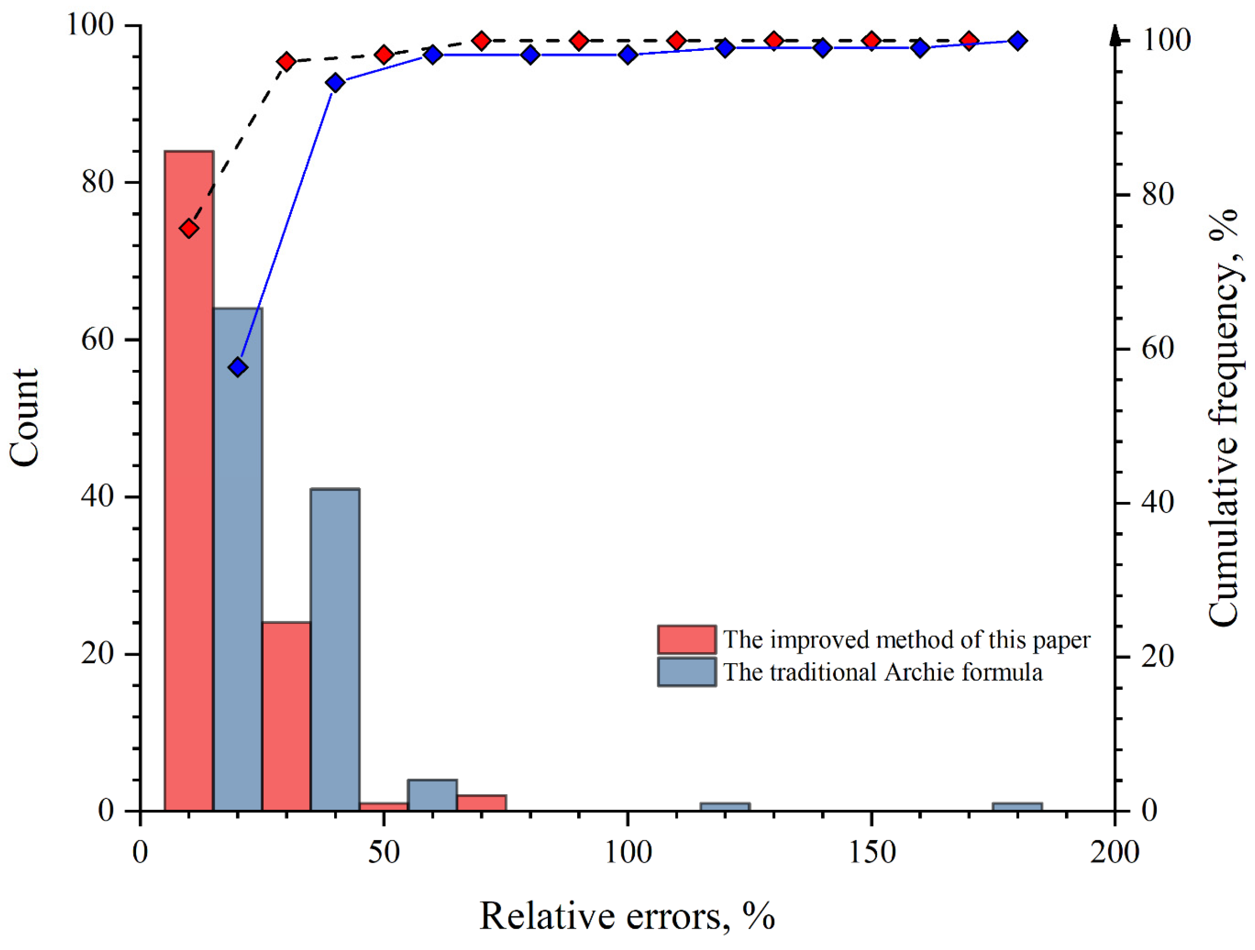
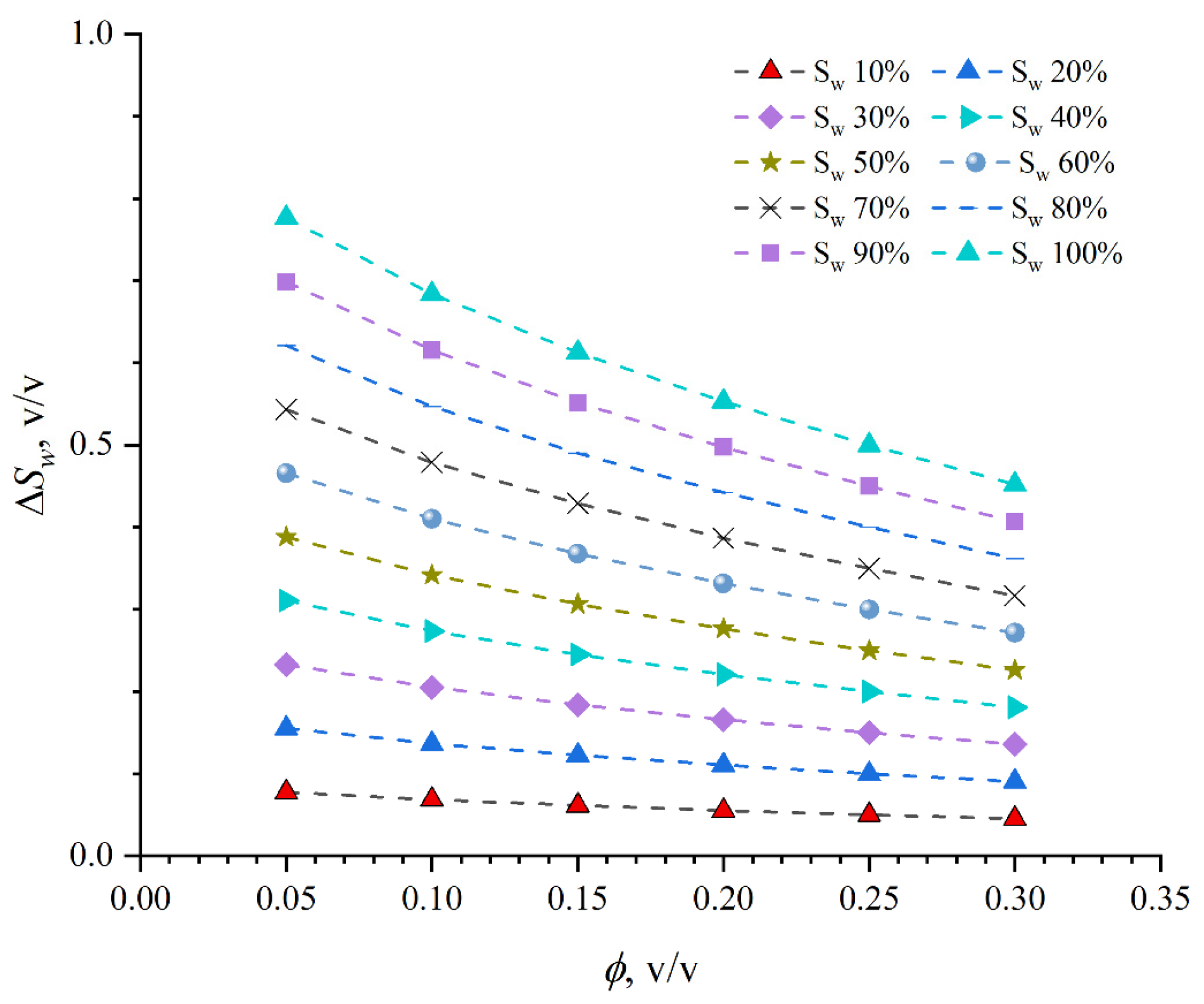
4.3.1. The Error Analysis of Water Saturation

The irreducible water saturation is predicted by the machine learning method combined with geophysical logging data, and the curves involved in the prediction use conventional logging data. The calculation error of irreducible water saturation mainly originates from the algorithm itself and the acquisition error of geophysical logging data. For the geophysical logging curves, the acquisition process is affected by the borehole environment and human construction factors; there are inevitable human errors in the post-coring MICP experiments and core data acquisition experiments. In the actual data involved in the model construction, samples that do not meet industry standards and laboratory requirements are eliminated, considering that it is difficult to construct a separate model for elimination of various errors; thus, we assume no errors at input and the increase in errors at output [44]. In the demonstration of the actual wells, such errors are found to be within acceptable limits by comparing the calculated results with the core results, especially in the oil layers where the calculated results of irreducible water saturation are in good agreement with the water saturation and are further validated against each other.

For water saturation, the source of error is similar to that of irreducible water saturation. In addition to the error of core experimental data and the acquisition error of logging data, there are also errors in the transfer of intermediate parameters, such as the calculation of porosity. The porosity is calculated using the neutron-density rendezvous method, which, though widely used, is known to have errors. In Figure 15, when the evaluation error of porosity increases, the calculation error of water saturation also increases significantly compared to the irreducible water saturation, which is less affected. When the calculation result of porosity is high, the calculation result of water saturation is low; meanwhile, the response of the resistivity curve is also influenced by many factors, such as formation steady pressure, surrounding rock, pore structure, etc., which are difficult to eliminate one by one; thus, is also one of the sources of the evaluation error of water content saturation.

The traditional Archie formula (Equation (3)) can be taken logarithmically for both sides simultaneously to obtain the following:

$$\ln S_w=-\frac{1}{n}\ln R_t-\frac{m}{n}\ln \varphi +\frac{1}{n}\ln (ab{R}_w)$$

(21)

At this point, the reservoir water saturation calculated using Equation (21) is considered to be the exact value; when the error of the cementation index is $\pm c$, the calculated water saturation is as follows:

$$\ln S_w^{\prime }=-\frac{1}{n}\ln R_t-\frac{m\pm c}{n}\ln \varphi +\frac{1}{n}\ln (ab{R}_w)$$

(22)

According to the actual cementation situation and using the traditional Archie formula, $m$ is taken as 1.7; however, in this experiment, $m$ can reach up to 2.4; at this time the assumption error $c$ is 0.5. By combining Equation (21) with Equation (22), the reservoir water content saturation can be calculated as

$$\Delta S_w=\left|S_w^{\prime }-S_w\right|=\left|({\varphi }^{\mp 0.5}-1)S_w\right|$$

(23)

Combined with the actual data situation of the M layer group in the study area, the parameters were taken according to the corresponding ones in Table 2, and the calculation errors were explored for a porosity of 5–30% and a water content saturation distribution of 10–100%, as shown in Figure 16.

Combined with the actual situation, in low porosity reservoirs, the cementation index takes a small value. The higher the water saturation, the larger the corresponding theoretical error, and with the increase in porosity, this error tends to decrease on the whole, which is consistent with the existing investigation conclusions [25]. In other words, for low porosity reservoirs, the $m$ value will greatly affect the calculation of the water saturation of the reservoir, and the resistivity response value is affected by many factors. This is the reason why the traditional Archie formula often results in large errors in the evaluation of low porosity reservoirs, which also leads the water saturation of low porosity reservoirs to exceed 100%.

In terms of the final evaluation effect, the improved water saturation evaluation method in this paper avoids the selection of the crossover index compared with the traditional Archie formula; improvement results from fitting the model more accurately, achieving a more stable application effect.

4.3.2. Advantages of the Total Differential Method

The proposed fluid property identification method is based on a modified Archie formula, which takes into account the variation of resistivity, porosity, water saturation, and irreducible water saturation when identifying fluid properties. In addition, the differential form further amplifies the response of fluid properties to geophysical logging data through mathematical calculations. This paper points out the disadvantages of the quick method commonly used in the field, which can be analyzed using the principle of drilling fluid intrusion: Under freshwater drilling fluid conditions, because the resistivity of drilling fluid filtrate is greater than the resistivity of formation water, when the fluid filtrate permeates the water layer, the resistivity of the flushing zone increases, and high invasion will occur. When the drilling fluid filtrate permeates the oil layer and drives away the movable oil, low invasion will occur because the drilling fluid filtrate resistivity is smaller than the oil resistivity. Figure 17a shows the resistivity intrusion of different fluid properties in the M formation with RD greater than RXO in the oil layer and the opposite in the water layer, which is consistent with the intrusion characteristics. However, it is difficult to establish accurate boundaries for the transition zones; in particular, the boundary between the transition zone and the water layer is not obvious nor is the boundary between the oil layer and the transition zone.

The intrusion characteristics can be used to quickly identify oil and water layers in the reservoir, but the identification accuracy is low. The RXO is influenced by mud filtrate and construction factors, which also limits the accuracy of this method; thus, it is mostly used for rapid interpretation in the field. Similar to the above method, the rendezvous using water saturation and irreducible water saturation can also be used for reservoir fluid property identification; comparing the magnitude of the two can determine whether there is movable water in the reservoir. Figure 17b shows the water saturation and irreducible water saturation for different fluid properties in the M formation group. The water saturation of the oil layer and irreducible water saturation are similar; due to the error of the evaluation method itself, the two cannot be exactly equal. In the transition zone and water layer, the water saturation will be higher than the irreducible water saturation, indicating that there is movable water in the reservoir; however, similar to the intrusion method, the characteristics of the transition zone have no obvious demarcation line compared with the water layer, and interpretation is necessary for delineation. The error of the saturation calculation itself also increases the instability. In contrast, the total differential method can describe the thickness of the transition zone more accurately through the oil layer discriminant line and the water layer discriminant line.

Similarly, this paper compares the effectiveness of the traditional differential method with the improved total differential method for fluid identification applications. The traditional differential method is presented in Section 3.2, specifying two sets of judgment criteria based on the differential method of porosity and water saturation. This method is improved in this paper by differentiating both porosity and water saturation to address the tediousness of evaluation. Figure 18 shows well E in the study area where the eighth track is the total differential method used in this paper, and the ninth and tenth tracks are the results of the discriminant results of the traditional differential method of differentiating porosity from water saturation. In the fluid property identification results of MC1_1, there are differences between the two methods, and the two sets of discrimination results of the traditional differential method are not unified. The results of differential differentiation of porosity indicate that this section may be a transition zone, and the reservoir already contains water, while the results of differential differentiation of water saturation indicate that this is an oil layer. The total differential method simplifies the discrimination criterion and gives an ODT of −3085 m, which is consistent with the results of the traditional differential method for water saturation; combined with the DST result, this indicates that this is an oil layer. In contrast, the risk of discriminatory contradiction may occur in the practical application of the traditional differential method, while the total differential method considers multiple parameters simultaneously and amplifies this response trend, making the improved total differentiation method more stable and practical.

4.3.3. Limitations of the Total Differential Method

The total differential method also has certain risks and limitations in its practical use, including the following:

1. The total differential method relies on the calculation accuracy of the water saturation and the irreducible water saturation as input-type parameters, and the accuracy of the evaluation of the two saturations will affect the application effect of the total differential method. In the oil layer, the water saturation and the irreducible water saturation should theoretically coincide with one another. From the actual evaluation results, Figure 17b shows that they generally coincide, but there is some error, which has been pointed out in the error analysis of water saturation in previous studies. In addition, the values and patterns of water saturation and irreducible water saturation are nearly the same for the oil layer in Figure 12. The calculated line is parallel to the oil formation discriminant line after being enlarged by the total differential method, which is filled with blue color but has no increasing trend; thus, it can still be effectively judged as an oil layer. Similarly, when indicating the water layer, the calculated line and the water layer discriminant line may not coincide exactly; when the two are parallel and the blue filling no longer increases, the water layer can be determined. The evaluation error of water saturation and irreducible water saturation makes it difficult to use both saturations, while the total differential method amplifies the numerical relationship between the two by means of differentiation, combining porosity, rock-electric parameters, etc. It no longer depends entirely on the calculation of both saturations, making the method more stable and easier to use compared to the traditional differential method.

2. Geophysical logging data from open-hole wells are not sustainable in identifying reservoir fluid properties. Compared with casing-hole logging data, logging data from open-hole wells reflect reservoir fluid properties at the time of logging. If a long period of time elapses after logging before production, the reservoir fluid properties will change significantly with the development of the field, and the ODT and WUT will be elevated as bottom and edge waters continue to fall in. Taking the 22 wells in the study block as an example, these wells, logged from 2011 to 2023, are logged close to the production time and are less affected. It can be seen from Figure 19 that the TVDSS of ODT is about −30 58 m from 2011 to 2014, which is the original reservoir lower interface; with the development of the M formation group in the H field, the ODT started to lift in 2017, and the lifting trend has been gradually increasing since then.

Although the total differential method has some limitations, it is simple to calculate and highly accurate compared to previous evaluation tools and has more prominent practicality for rapid interpretation in the field.

4.3.4. Future Trends

In this paper, the analysis of geological and experimental data reveals that the traditional Archie formula is not applicable. To improve the formula, this paper illustrates it from the mathematical point of view; however, a more in-depth study can be conducted physically, and further research on the conductivity mechanism can be carried out, for example, by analyzing the conductivity porosity. In addition, for reservoir fluid property identification, in addition to relying on the validity of the water saturation calculation, the improvement of the irreducible water saturation calculation can also be studied in more depth.

5. Conclusions

In this paper, the Archie formula is improved for calculating water saturation by taking the M formation group in the H field as an example, and a new reservoir fluid property identification method is proposed based on the improved formula. The following conclusions are obtained:

(1)

The application of the traditional Archie formula in the M formation of the H oil field is limited by the complex pore structure of the block, and the direct use effect is poor. The relationship between formation factors and porosity determined by a mathematical fitting method is proposed. Based on this, an improved Archie formula is proposed to calculate water saturation. The water saturation calculated by the improved formula has higher accuracy and applicability, avoiding the problem of taking the value of the cementation index in the traditional Archie formula.

(2)

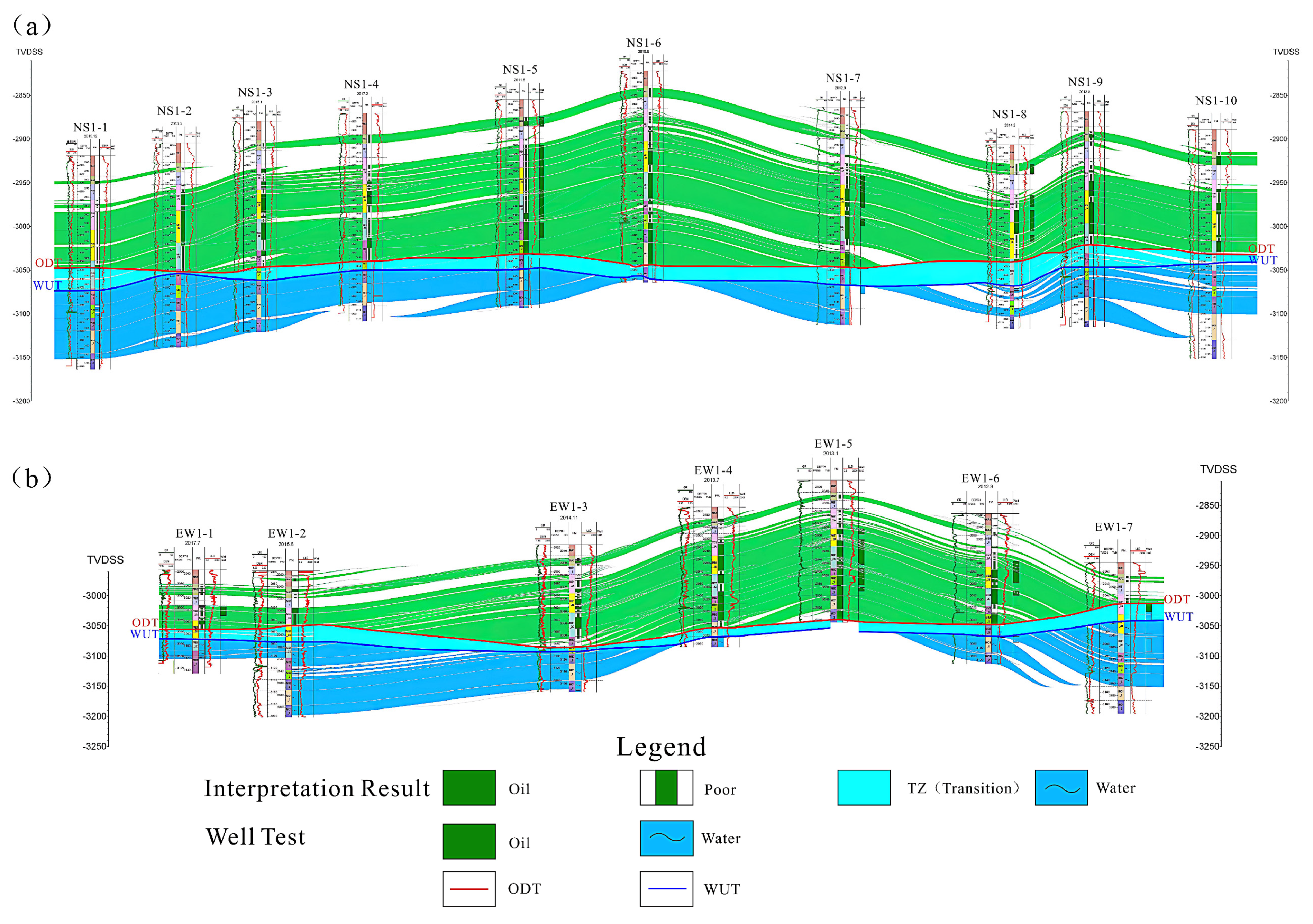
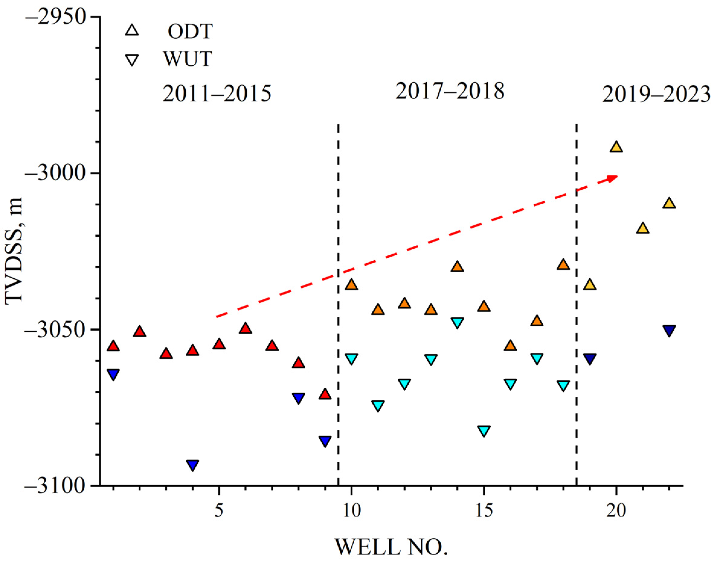
Based on the improved Archie formula, the total differential method is proposed to identify the reservoir fluid properties; based on the resistivity, the porosity and water saturation are differentiated, and the resistivity variation characteristics are amplified by the petrophysical parameters. The oil discriminant line is compared with the water discriminant line to identify the reservoir fluid properties, which achieves good results in the target block M formation. Compared with the intrusion method and the saturation comparison method, the full differential method is more systematic for the identification of ODT and WUT; this method is easier to use than the traditional differential method and avoids the risk of contradiction in identification.

(3)

Compared with the casing-hole data, the open-hole well data cannot continuously monitor the change in reservoir fluid properties. In the face of wells with similar logging time and production time, the total differential method is applicable and can compare the logging data of different periods to construct oil–water profiles of different time periods to observe the change in ODT so as to allow adjustment on the production scheme to increase the production.

Relying on actual experimental data, this paper improves the water saturation calculation formula in combination with Archie’s formula and proposes a new set of reservoir fluid property identification methods based on the improved formula. The method in this paper is suitable for field application and can meet the requirements of evaluating the water saturation of the M formation group in the study area. At the same time, the method is inexpensive to calculate, easy to implement, and can be directly linked to professional software. Meanwhile, the work of this paper also provides a new method for rapid identification of reservoir fluid properties in oil fields, which has practical application value.

References

1. Roehl, P.O.; Choquette, P.W. (Eds.) Carbonate Petroleum Reservoirs; Springer Science & Business Media: Berlin/Heidelberg, Germany, 2012; pp. 1–15. [Google Scholar]
2. Carvalho, Á.; Dias, A.; Ribeiro, M.T. Oil recovery enhancement for Thamama B Lower in an Onshore Abu Dhabi Field. Using conceptual models to understand reservoir behaviour. In Proceedings of the SPE Reservoir Characterisation and Simulation Conference and Exhibition, Abu Dhabi, United Arab Emirates, 9 October 2011. [Google Scholar]
3. Nairn, A.E.M.; Alsharhan, A.S. Sedimentary Basins and Petroleum Geology of the Middle East; Elsevier: Amsterdam, The Netherlands, 1997; pp. 1–942. [Google Scholar]
4. Gao, J.; Tian, C.; Zhang, W.; Song, X.; Liu, B. Characteristics and genesis of carbonate reservoir of the Mishrif Formation in the Rumaila oil field, Iraq. Acta Pet. Sin. 2013, 34, 843–852. [Google Scholar]
5. Thong, X.; Zhang, G.; Wang, Z.; Wen, Z.; Tian, Z.; Wang, H.; Ma, F.; Wu, Y. Distribution and potential of global oil and gas resource. Pet. Explor. Dev. 2018, 45, 727–736. [Google Scholar] [CrossRef]
6. Kang, Y. Status of world hydrocarbon resource potential and strategic thinking of overseas oil and gas projects for China. Nat. Gas Ind. 2013, 33, 1–4. [Google Scholar]
7. Zhang, X.; Pang, X.; Jin, Z.; Hu, T.; Toyin, A.; Wang, K. Depositional model for mixed carbonate-clastic sediments in the middle cambrian lower zhangxia formation, xiaweidian, north China. Adv. Geo Energy Res. 2020, 4, 29–42. [Google Scholar] [CrossRef]
8. Hu, Y.; Yu, X.; Chen, G.; Li, S. Classification of the average capillary pressure function and its application in calculating fluid saturation. Pet. Explor. Dev. 2012, 39, 733–738. [Google Scholar] [CrossRef]
9. Zhu, L.; Zhang, C.; Zhang, Z.; Zhou, X. High-precision calculation of gas saturation in organic shale pores using an intelligent fusion algorithm and a multi-mineral model. Adv. Geo Energy Res. 2020, 4, 135–151. [Google Scholar] [CrossRef]
10. Archie, G. The electrical resistivity log as an aid in determining some reservoir characteristics. Trans. AIME 1942, 146, 54–62. [Google Scholar] [CrossRef]
11. Serra, O. Formation MicroScanner Image Interpretation; Schlumberger Educational Services: Houston, TX, USA, 1989. [Google Scholar]
12. Wang, M. Improvement and analysis of carbonate reservoir saturation model. J. Southwest Pet. Univ. Sci. Technol. Ed. 2013, 35, 31–40. [Google Scholar]
13. Aguilera, R. A triple porosity model for petrophysical analysis of naturally reservoirs. Petrophysics 2004, 45, 157–166. [Google Scholar]
14. Fleury, M. Resistivity in carbonates: New insights. In Proceedings of the SPE Annual Technical Conference and Exhibition, San Antonio, TX, USA, 29 September 2002. [Google Scholar]
15. Fleury, M.; Efnik, M.; Kalam, M. Evaluation of water saturation from resistivity in a carbonate field from laboratory to logs. In Proceedings of the International Symposium of the Society of Core Analysts, Abu Dhabi, United Arab Emirates, 5–9 October 2004. [Google Scholar]
16. Kazatchenko, E.; Markov, M.; Mousatov, A.; Pervago, E. Simulation of the electrical resistivity of dual-porosity carbonate formations saturated with fluid mixtures. Petrophysics 2006, 47, 23–36. [Google Scholar]
17. Pan, H.; Wang, X.; Fan, Z.; Ma, Y.; Li, M. Computing method of reservoir originality oil saturation. Geoscience 2000, 14, 451–453. [Google Scholar]
18. Leverett, M. Capillary behaviors in porous solids. Trans. AIME 1941, 142, 152–169. [Google Scholar] [CrossRef]
19. Purcell, W. Capillary pressures-their measurement using mercury and the calculation of permeability therefrom. J. Pet. Technol. 1949, 1, 39–48. [Google Scholar] [CrossRef]
20. Zeng, W.; Liu, X. Interpretation of non-Archie phenomenon for carbonate reservoir. Well Logging Technol. 2013, 37, 151–341. [Google Scholar]
21. Mungan, N.; Moore, E. Certain wettability effects on electrical resistivity in porous media. J. Can. Pet. Technol. 1968, 7, 20–25. [Google Scholar] [CrossRef]
22. Simandoux, P. Dielectric measurements of porous media: Application to measurement of water saturations, study of the behavior of argillaceous formations. Rev. L’Inst. Fr. Pet. 1963, 18, 193–215. [Google Scholar]
23. Tian, H.; Li, C.; Jia, P. Research of water saturation interpretation models for carbonate reservoir. Prog. Geophys. 2017, 32, 279–286. [Google Scholar]
24. Senden, T.; Sheppard, A.; Kumar, M.; Knackstedt, M.; Arns, C. Variations in the Archie? s exponent: Probing wettability and low Sw effects. In Proceedings of the SPWLA 51st Annual Logging Symposium, Perth, Australia, 19 June 2010. [Google Scholar]
25. Li, X.; Qin, R.; Liu, C. Analyzing the Effect of Rock Electrical Parameters on the Calculation of the Reservoir Saturation. J. Southwest Pet. Univ. Sci. Technol. Ed. 2014, 36, 68–74. [Google Scholar]
26. Li, Y.; Zhang, Z.; Hu, S.; Zhou, X.; Guo, J.; Zhu, L. Evaluation of irreducible water saturation by electrical imaging logging based on capillary pressure approximation theory. Geoenergy Sci. Eng. 2023, 224, 211592. [Google Scholar] [CrossRef]
27. Kumar, M.; Senden, T.; Arns, C.; Sheppard, A.; Knackstedt, M. Probing the Archie’s exponent under variable saturation conditions. Petrophysics 2011, 52, 124–134. [Google Scholar]
28. Sun, J.; Wang, K.; Li, W. Development and analysis of logging saturation interpretation models. Pet. Explor. Dev. 2008, 35, 107–113. [Google Scholar]
29. Zhang, M.; Qiao, Z.; Gao, J.; Zhu, Y.; Sun, W. Characteristics and evaluation of carbonate reservoirs in restricted platform in the MB1-2 Sub-Member of Mishrif formation, Halfaya oilfield, Iraq. J. Northeast Pet. Univ. 2020, 44, 35–45. [Google Scholar]
30. Alsharhan, A.; Nairn, A. A review of the Cretaceous formations in the Arabian Peninsula and Gulf: Part I. Lower Cretaceous (Thamama Group) stratigraphy and paleogeography. J. Pet. Geol. 1986, 9, 365–391. [Google Scholar] [CrossRef]
31. Alsharhan, A.; Nairn, A. A review of the ctretaceous formations in the Arabian peninsula and gulf: Part II. Mid-cretaceous (Wasia Group) stratigraphy and paleogeography. J. Pet. Geol. 1988, 11, 89–112. [Google Scholar] [CrossRef]
32. Sadooni, F.; Alsharhan, A. Stratigraphy, microfacies, and petroleum potential of the Mauddud Formation (Albian-Cenomanian) in the Arabian Gulf basin. AAPG Bull. 2003, 87, 1653–1680. [Google Scholar] [CrossRef]
33. Dunham, R. Classification of carbonate rocks according to depositional textures. In Classification of Carbonate Rocks—A Symposium; AAPG Datapages Inc.: Tulsa, OK, USA, 1962; Volume 1, pp. 108–121. [Google Scholar]
34. Lucia, F. Petrophysical parameters estimated from visual descriptions of carbonate rocks: A field classification of carbonate pore space. J. Pet. Technol. 1983, 35, 629–637. [Google Scholar] [CrossRef]
35. Jebbouri, A.; Belhaj, H.; Khalifeh, H.; Naik, M. Investigation of Depletion Process Influence on Relative Permeability and Residual Oil Saturation of Thick TZ Carbonate Reservoir. In Proceedings of the SPE Middle East Oil & Gas Show and Conference, Manama, Bahrain, 8 March 2015. [Google Scholar]
36. Li, J.; Zhang, C.; Tang, W.; Li, J.; Xiao, C. Major influential factor and quantitative study on m exponent and n exponent in Kuche Region. J. Oil Gas Technol. 2009, 31, 100–103. [Google Scholar]
37. Zhang, W. Identification Methods Study on Fluid Property of Complex Reservoirs. Master’s Thesis, China University of Petroleum, Qingdao, China, 2011; pp. 33–36. [Google Scholar]
38. El-Bagoury, M. Integrated petrophysical study to validate water saturation from well logs in Bahariya Shaley Sand Reservoirs, case study from Abu Gharadig Basin, Egypt. J. Pet. Explor. Prod. Technol. 2020, 10, 3139–3155. [Google Scholar] [CrossRef]
39. Ma, M.; Li, J. A correction of oil-and water-saturation obtained from sealed core analysis. Pet. Explor. Dev. 1993, 20, 102–105. [Google Scholar]
40. Guo, J.; Zhang, Z.; Guo, G.; Xiao, H.; Zhu, L.; Zhang, C.; Tang, X.; Zhou, X.; Zhang, Y.; Wang, C. Evaluation of Coalbed Methane Content by Using Kernel Extreme Learning Machine and Geophysical Logging Data. Geofluids 2022, 2022, 3424367. [Google Scholar] [CrossRef]
41. Zhang, Q.; Wei, C.; Wang, Y.; Du, S.; Zhou, Y.; Song, H. Potential for Prediction of Water Saturation Distribution in Reservoirs Utilizing Machine Learning Methods. Energies 2019, 12, 3597. [Google Scholar] [CrossRef]
42. Breiman, L.; Cutler, A. Random forests. Mach. Learn. 2001, 45, 5–32. [Google Scholar] [CrossRef]
43. Breiman, L. Bagging predictors. Mach. Learn. 1996, 24, 123–140. [Google Scholar] [CrossRef]
44. Zhou, B.; O’Brien, G. Improving coal quality estimation through multiple geophysical log analysis. Int. J. Coal Geol. 2016, 167, 75–92. [Google Scholar] [CrossRef]
Figure 1. Location of the H field study area and geological overview of the M formation group.
Processes 11 01282 g001
Figure 2. Lithological frequency distribution in the study area: (a) the percentage of limestone and dolomite in the study area and (b) distribution of various types of limestone in the study area based on Dunham’s limestone classification criteria.
Processes 11 01282 g002
Figure 3. Mineral content and pore type distribution in the study area: (a) the mineral content of the study area (XRD); (b) the distribution trend of the mineral content in the study area; and (c) the pore type distribution of the study area.
Processes 11 01282 g003
Figure 4. Core cementation index analysis chart of 89 blocks in M layer group of H oil field: (a) the distribution of cementation index ( m ) values of cores and (b) the distribution proportion of cementation degree of cores. The navy blue dots in this figure are the values of the formation factors and porosity for each sample in the rock-electric experiment.
Processes 11 01282 g004
Figure 5. The fitting relationships between formation factors and porosity: (a) traditional fitting method and (b) the fitting method of this paper. The green dots in Figure 5a show the values of the formation factors and porosity for each sample in the rock-electric experiment. A and B and the corresponding circles are the two partitions. The dashed line is the result of the fit, used for parameter determination.
Processes 11 01282 g005
Figure 6. The relationship between resistivity increase coefficient and water saturation of 49 cores in the M formation of the H oil field. The yellow triangles in the figure show the relationship between the resistance increase coefficient and the different water saturation in the rock-electric experiment.
Processes 11 01282 g006
Figure 7. Comparison of calculation results with core results: (a) the calculation results of the method in this paper and (b) the calculation results of the traditional Archie’s formula. The solid line in Figure 7 is the zero-error line, and the red dotted line is the trend line of the fit of the calculated results to the core data. The origin is the projection of the calculated results with the core results.
Processes 11 01282 g007
Figure 8. The histogram of the relative errors of the two methods. The red and navy blue lines in the figure correspond to the cumulative distribution curves of the errors of the water saturation calculated by the method of this paper and the traditional Archie’s Archie formula, respectively, and the solid points represent different ranges.
Processes 11 01282 g008
Figure 9. Comparison of the calculated results of irreducible water saturation with the core results: (a) calculated results for the training dataset and (b) calculated results for the test dataset. The solid line in Figure 9 is the zero-error line, and the red dotted line is the trend line of the fit of the calculated results to the core data. The origin is the projection of the calculated results with the core results.
Processes 11 01282 g009
Figure 10. The calculation results of water saturation of reservoir in well A.
Processes 11 01282 g010
Figure 11. The calculation results of water saturation of reservoir in well B.
Processes 11 01282 g011
Figure 12. Identification results of reservoir fluid properties in well C based on total differential method.
Processes 11 01282 g012
Figure 13. East–west and south–north oil–water profile well location diagrams in the work area.
Processes 11 01282 g013
Figure 14. The calculation results of east–west and south–north oil-water profiles in the M layer group: (a) south–north direction and (b) east–west direction.
Processes 11 01282 g014
Figure 15. The water saturation evaluation results in well D.
Processes 11 01282 g015
Figure 16. The influence of different cementation indexes on water saturation error.
Processes 11 01282 g016
Figure 17. The results of reservoir fluid property identification using traditional methods: (a) resistivity intrusion method and (b) water saturation and irreducible water saturation intersection method.
Processes 11 01282 g017
Figure 18. The difference between the traditional total differential method and the method used in this paper in the identification of fluid properties (taking well E as an example).
Processes 11 01282 g018
Figure 19. With the recommendation of oil field development time, the change diagram of ODT and WUT is calculated by geophysical logging data. The transformation of the three colors represents the different development periods of H oil field. From left to right, the colors used in different development stages are different. The turning points are indicated by the triangles; the positive triangle is ODT, and the inverted triangle is WUT.
Processes 11 01282 g019