Time Series-Based Edge Resource Prediction and Parallel Optimal Task Allocation in Mobile Edge Computing Environment

Abstract

The offloading of computationally intensive tasks to edge servers is indispensable in the mobile edge computing (MEC) environment. Once the tasks are offloaded, the subsequent challenges lie in buffering them and assigning them to edge virtual machine (VM) resources to meet the multicriteria requirement. Furthermore, the edge resources’ availability is dynamic in nature and needs a joint prediction and optimal allocation for the efficient usage of resources and fulfillment of the tasks’ requirements. To this end, this work has three contributions. First, a delay sensitivity-based priority scheduling (DSPS) policy is presented to schedule the tasks as per their deadline. Secondly, based on exploratory data analysis and inferred seasonal patterns in the usage of edge CPU resources from the GWA-T-12 Bitbrains VM utilization dataset, the availability of VM resources is predicted by using a Holt–Winters-based univariate algorithm (HWVMR) and a vector autoregression-based multivariate algorithm (VARVMR). Finally, for optimal and fast task assignment, a parallel differential evolution-based task allocation (pDETA) strategy is proposed. The proposed algorithms are evaluated extensively with standard performance metrics, and the results show nearly 22%, 35%, and 69% improvements in cost and 41%, 52%, and 78% improvements in energy when compared with MTSS, DE, and min–min strategies, respectively.

1. Introduction

With the increasing popularity of mobile user equipment and the evolution of 5G/6G-enabled wireless communication, users are attracted to applications that are computationally intensive in nature, e.g., image-processing applications, augmented reality (AR)-, and virtual reality (VR)-based applications, etc. [1,2]. Mobile equipment with limited computational capacity and restricted battery power fail to meet the requirements of these applications. In recent years, the emerging paradigm of mobile edge computing (MEC), which is also regarded as the successor to mobile cloud computing (MCC), helps to alleviate such problems pertaining to the resource limitations of mobile equipment. This is achieved by providing a computing facility in close proximity to the users, under the computation offloading services, so that the users can offload their application tasks to the MEC servers for the computation and can download their results back to their respective mobile devices [3,4].

The computation offloading service has been shown tremendous interest by academia and industry in the last few decades [5,6] due to advancements in smart devices and in wireless communication technologies like 5G/6G, which makes offloading a reality. At the same time, this service has faced several open challenges at the user level or device layer as well as at the server level or edge layer, which is the current trend of research in the field of MEC [7,8]. The first and foremost issue is making a suitable decision with regard to whether the offloading is beneficial for the user or not and whether to offload a complete set of tasks or to partition tasks based on their dependencies [9,10].

Secondly, once the tasks are offloaded to the MEC server, the subsequent challenges lie in buffering the tasks by considering various task-oriented parameters, e.g., deadline, delay sensitivity, priority, energy consumption, etc., and assigning edge virtual machine (VM) resources to the tasks to meet various quality of service (QoS) requirements. Furthermore, the edge resources availability is time-varying in nature and needs a joint prediction and optimal allocation for efficient usage of resources and, at the same time, fulfillment of the parameters of the task.

Nevertheless, a plethora of work has recently been reported in the literature, focusing on the decision-making of computation offloading at the device layer [11,12] and assigning edge VM resources at the edge layer [13,14,15]. However, very few of these works have performed an exploratory datacenter resource-usage analysis to infer a temporal observation on the true usage of VM resources and accordingly devise a VM resource-assignment mechanism for user tasks [16]. Furthermore, when the number of offloaded tasks grows significantly, a fast resource-allocation mechanism needs to be in place for optimal resource usage and to meet the QoS requirements of mobile users.

To this end, the present work has focused on an in-depth exploratory analysis of VM resources of GWA-T-12 Bitbrain’s VM utilization dataset [17] and provided a time series-based edge resource prediction algorithm by using a Holt–Winters-based univariate algorithm (HWVMR) and a vector autoregression-based multivariate algorithm (VARVMR). Finally, for optimal and fast task assignment, a parallel differential evolution-based task allocation (pDETA) strategy is proposed.

The main contributions of this paper are as follows.

(i)

A delay sensitivity-based priority scheduling (DSPS) policy is presented to schedule the tasks as per their deadline.

(ii)

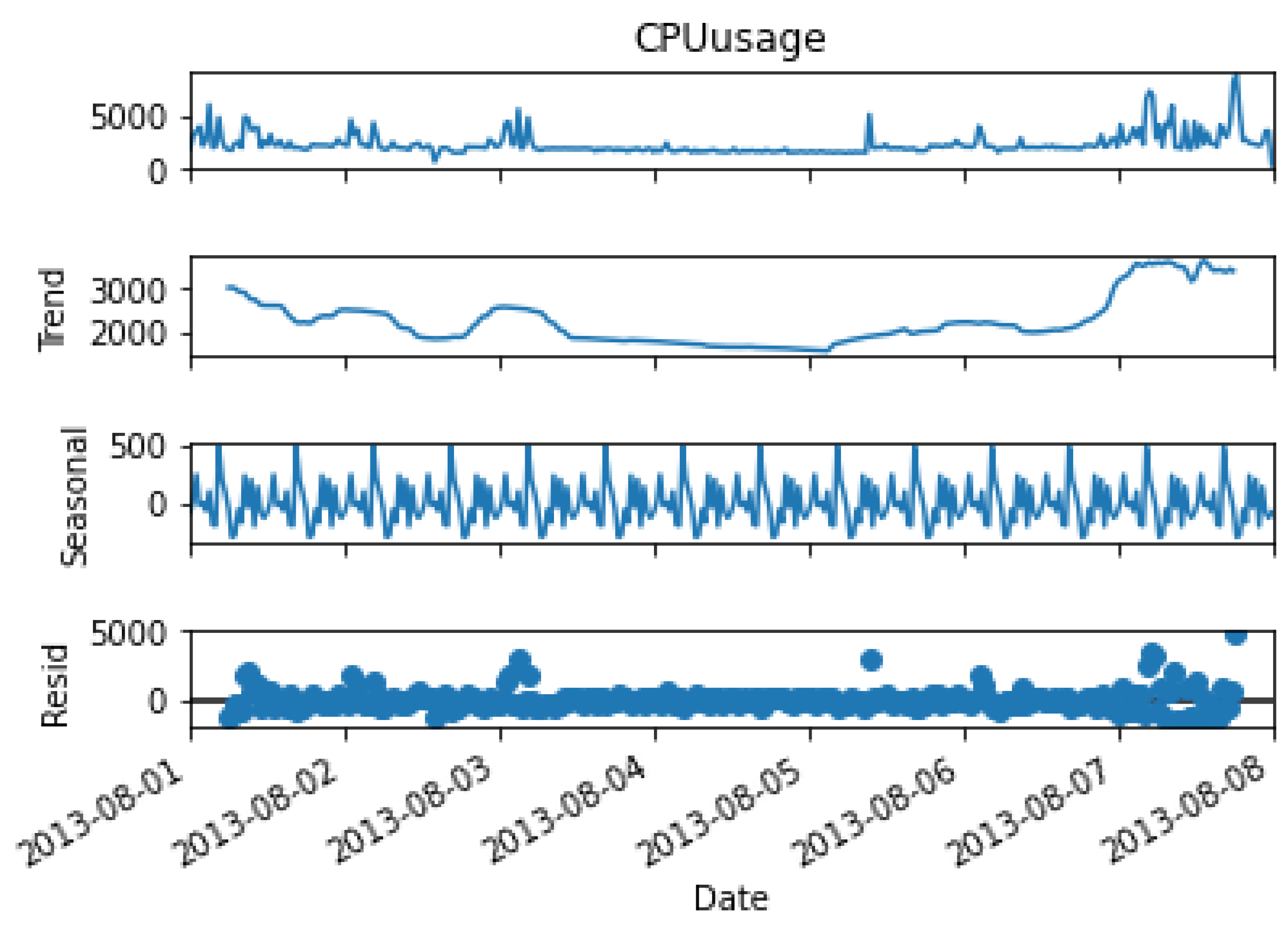
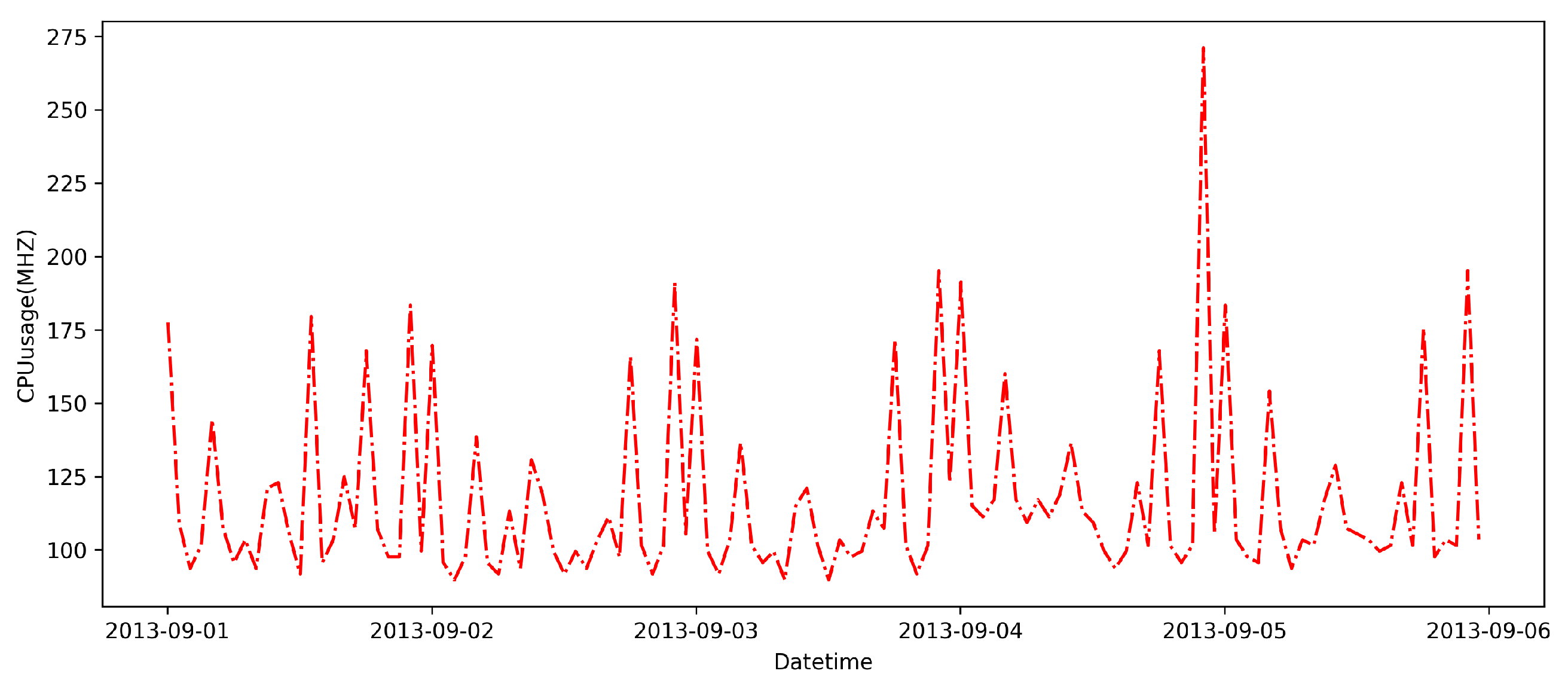
An exploratory data analysis is carried out, and inference is made regarding seasonal patterns in the usage of edge CPU resources from the GWA-T-12 Bitbrains VM utilization dataset.

(iii)

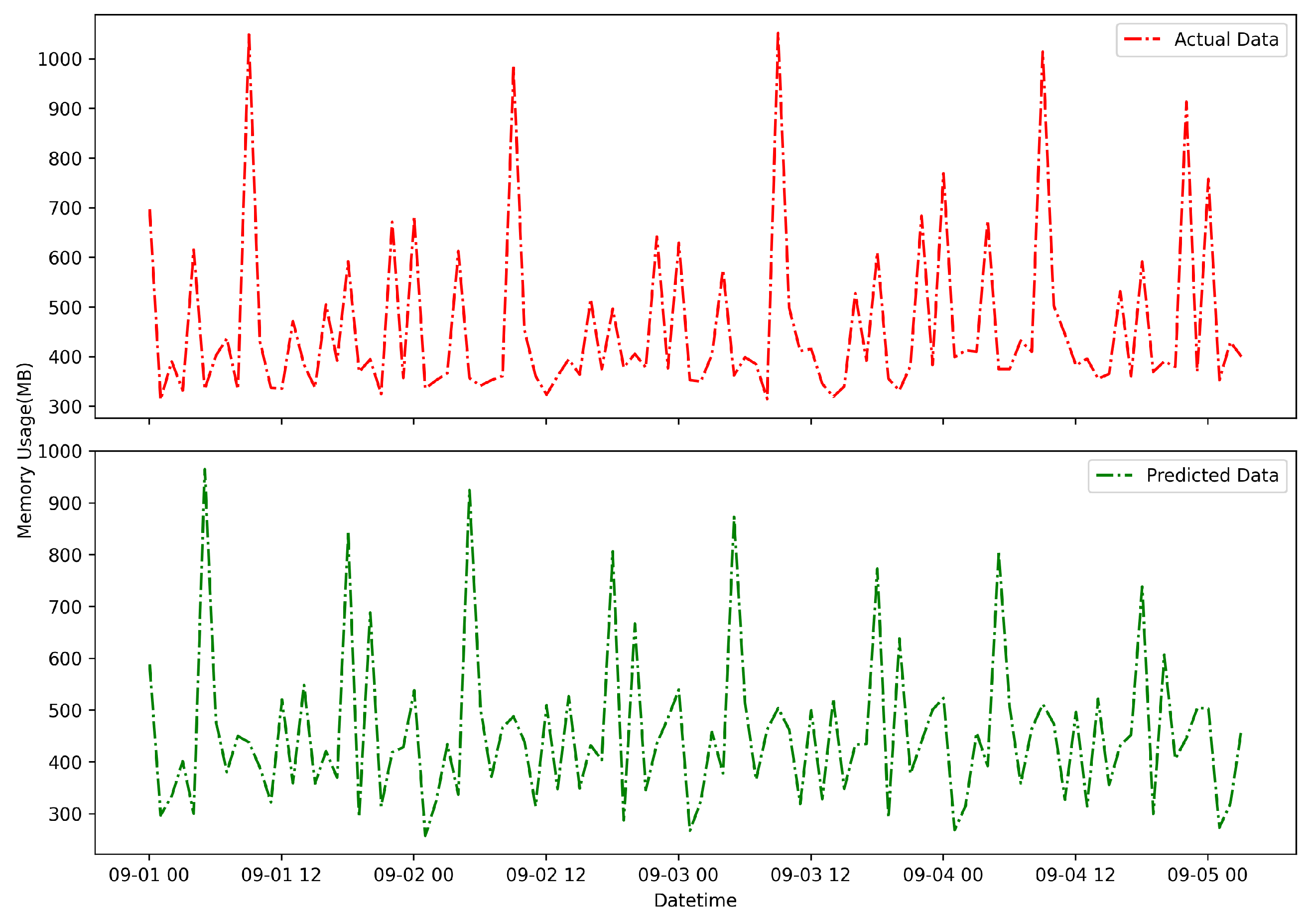
The availability of VM resources is predicted by using HWVMR and VARVMR.

(iv)

For optimal and fast task assignment, a parallel differential evolution-based task allocation (pDETA) strategy is proposed.

(v)

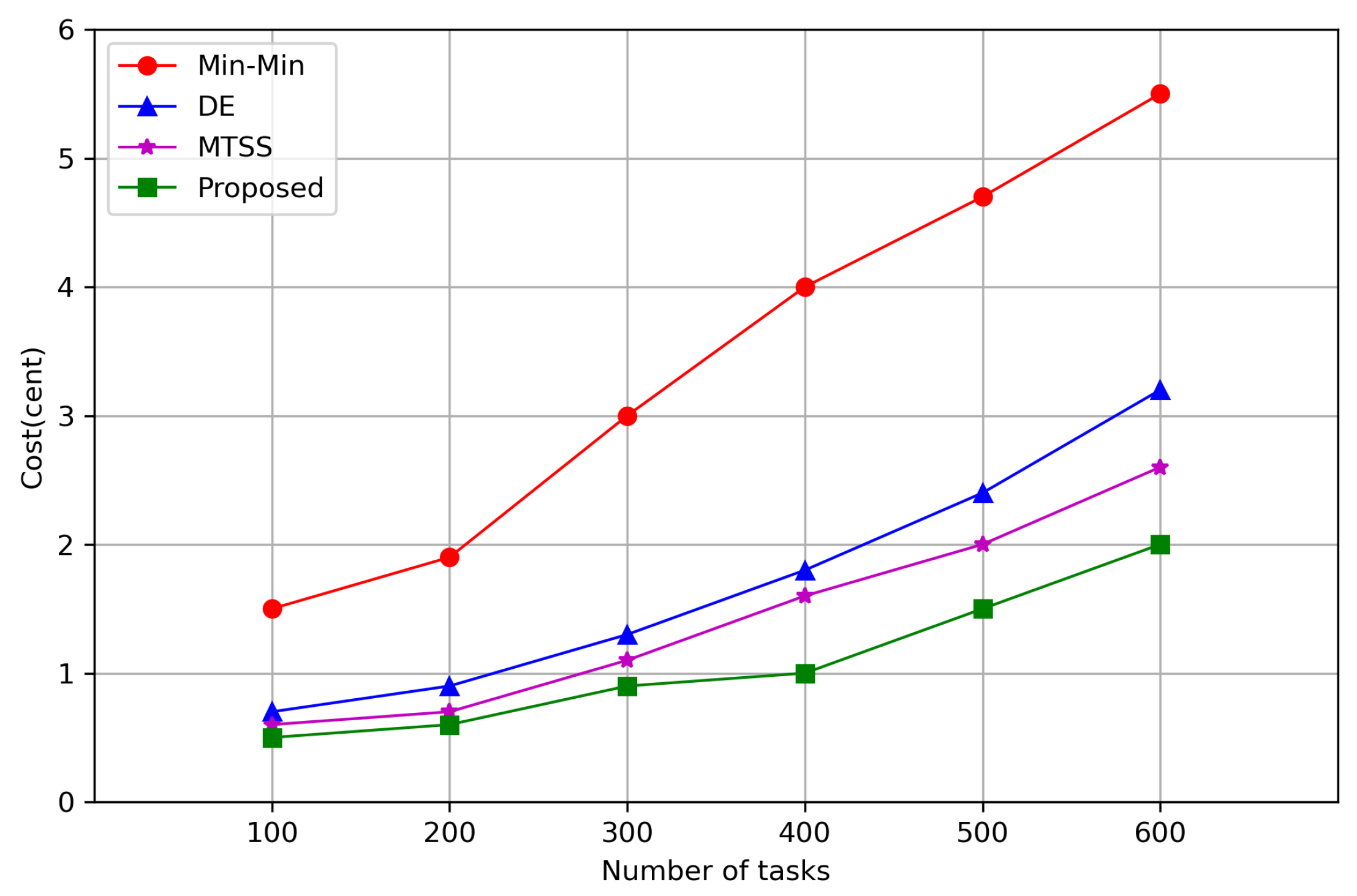
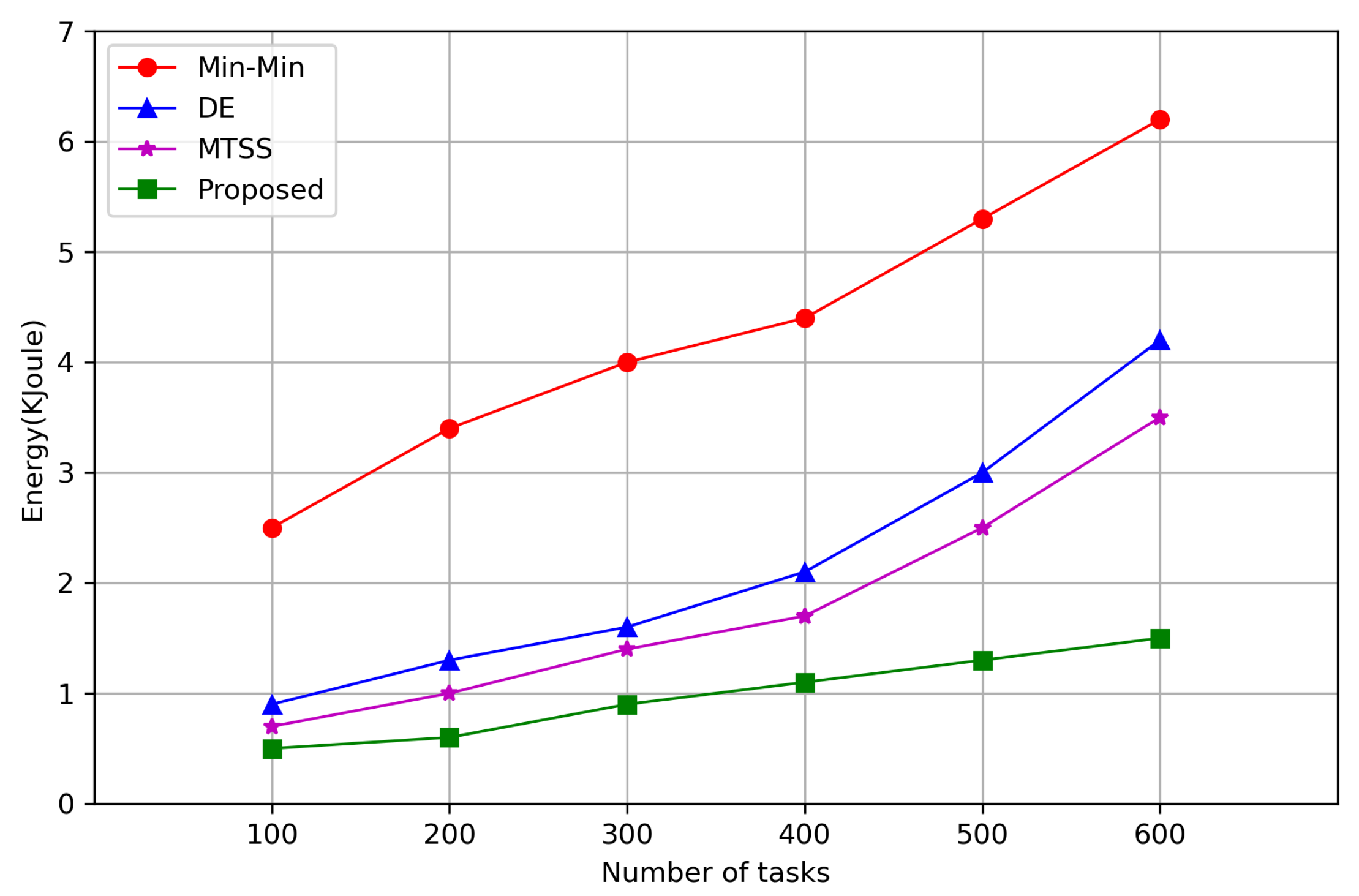
The proposed algorithms are evaluated extensively by using standard performance metrics, e.g., execution time, cost, and energy.

The rest of the paper is organized as follows: Section 2 highlights related work, Section 3 presents the various system models, Section 4 describes the problem statement, and Section 5 illustrates the proposed network architecture and task-execution process. The proposed strategies for scheduling, resource prediction, and parallel optimal resource allocation are presented under Section 6. Section 7 shows the simulation results, followed by a conclusion in Section 8.

2. Related Work

This section highlights some state-of-the-art works related to computation offloading problems in the MEC environment. The existing works can be broadly classified into three major domains: buffering/scheduling of offloaded tasks, prediction of edge VM resources, and VM resource allocation strategies.

Task buffering and scheduling policy is a prerequisite for offloaded tasks before they are placed in edge servers. In [18], the effects of different types of virtualization techniques for the edge computing concepts used in academics and the industry are discussed. Suitable scheduling and placement algorithms are used for the improvement of the response time, energy, cost, and better utilization of the VMs in edge computing. The authors have highlighted the security issues while using the VMs. In [19], considering task grouping and quadratic allocation, a service scheduling algorithm is proposed that ensures the reduction of the scheduling delay and server load balance, which improves the server utilization rate.

Time series analysis-based prediction for cloud resource usage has attracted many researchers. The CACTA [16] model helps to schedule the task, predict the resources, and allocate the task to the nearby edge nodes. The authors have considered the mobility, heterogeneity, and dynamics of the edge node, and the resource prediction is handled by time series analysis, with or without historical data. The completion time and system cost are minimized by using the Q-learning-based online assignment algorithm.

Considering the seasonal patterns, many papers deal with forecasting in faster ways. In [20], the authors have proposed the Holt–Winters formula for finding the initial forecasting, which results in better accuracy with fewer errors compared with the other models. In this proposal, the authors have considered different datasets for finding the best result $\alpha$, $\beta$, and $\gamma$. The multiple seasonal Holt–Winters methods [21] is proposed for better resource forecasting in the cloud environment. The authors have used the artificial bee colony algorithm to obtain optimal parameters. Their model worked well with the minimum number of observations. The model resulted in a significantly smaller percentage of errors in comparison with the double and triple exponential smoothing methods. Sarika et al. [22] describe the effectiveness of the resource usage prediction to avoid delays in VM. The authors have used time series forecasting for the prediction of CPU usage, memory usage, disk read time, and disk write time resources by considering univariate analysis. The authors have applied different time series models, such as ARIMA, SARIMA, Holt–Winters, and LSTM methods to the dataset and observed that the LSTM does not provide good results due to the smaller dataset and that Holt–Winters performs well. To minimize the delay while assigning the allocation of resources, Ouhame et al. [23] proposed a hybrid method by considering the multivariate situation by combining the VAR model with the LSTM model. The authors considered the two dependent metrics as CPU usage and memory usage from the dataset for calculating the multivariate time series. The authors produced experimental results to show the proposed hybrid model produces fewer errors in prediction as compared with the already existing combined models.

Docker technology [24] is used for better resource allocation with the task schedule in the edge gateway. This technology helps to schedule more tasks within less time, which results in a reduction in waiting time for the task and faster assignment to the resources. The authors proposed a greedy available fit model, which helps to reduce the data transmission latency. To utilize the resource optimally, the authors used an improved DE strategy [25]. The proposed algorithm MTSS used the benefits of the clustering method and made the clusters of the VMs and tasks. The proposed method results in the minimization of the execution cost, time, and workload and produced better results in resource utilization. In [26], the authors scheduled the cloud resources for their better utilization. The authors have proposed the multi-objective optimization algorithm, which performs better than the traditional GA and PSO algorithms. The proposed algorithm minimizes the cost and execution time and also results in better load balancing in cloud resources.

In [27], the authors proposed the fine-grained and coarse-grained models by using the parallel GA. The authors used several workstations for testing the models. They have considered the different sizes of the population and observed that when the population size increases, the number of iterations is decreased by using parallel models. The authors implemented the models by using the SCOOP method. The proposed model results in better computational time and reduced load balancing by effective utilization of the hardware. Yuanjun et al. [28] proposed a method for better scheduling and resource allocation of tasks by considering the cloud edge collaboration model. The authors made the different groups of correlated tasks. Then, by applying the evolutionary algorithm in a parallel manner, they assigned the requested tasks to the suitable resources once the resource allocation was complete. To form a solution, the sub-solutions were merged, which helps in the reduction of computation time and energy. Y. Sun et al. [29] proposed a differential evolution algorithm for an optimized system, which results in minimum energy consumption with a larger number of computation bits. The authors considered the computation bits for local computing as well as edge server computing. The authors have taken different energy consumption sources such as energy stations, edge servers, and the users during the offloading process, which results in a reduction in the energy-consumption process.

From the above study, we found that in scheduling strategies different papers highlight the major focus on arrival time, size of the task, and priority, but the delay sensitivity nature of the task is not considered as a priority. Many authors used different methods of time series-based prediction to predict the resource, but at the same time, they have not considered the univariate and multivariate time series analysis. As the prediction is fully dependent on the dataset, and consequently based on the dependent and independent nature of the parameters, the univariate and the multivariate time series analysis is required for the better prediction of the resource. Once the scheduling and prediction are successfully completed, many authors proposed the optimal allocation of the resource with the task by applying different optimized techniques without considering the parallel computation. With parallel computation, the allocation becomes faster than the conventional methods.

3. System Model

In this section, we have discussed the cost, energy, and load model based on the task and VM model. We consider a set of user devices as $UD$ = $\{U{D}_1,U{D}_2,\dots ,U{D}_n\}$ from which different sets of tasks are generated as T = $\{\{T_{11},T_{12},\dots ,T_{1m}\},\{T_{21},T_{22},\dots ,T_{2m}\}$, …, $\{T_{n1},T_{n2},\dots ,T_{nm}\}\}$. The tasks are computed in the edge server after receiving the requests from the user devices. The requested task is represented by using the task model as explained in Section 3.1. The tasks are computed in the available resources of the edge server. The resource is represented by using the VM model as explained in Section 3.2. The cost model, energy model, and load model of the system are discussed in Section 3.3, Section 3.4 and Section 3.5, respectively.

3.1. Task Model

The requested task is represented by different parameters as, T = {$T_s$, $D{S}_t$, B, $T_{CPU}$, $T_{MEM}$}, where $T_s$ is the size of the task, $D{S}_t$ is the delay sensitivity of the task, B is the required network bandwidth of the task, $T_{CPU}$ is the CPU rate required for the task, and $T_{MEM}$ is the memory required for the task. The task model is used to calculate the computation time of the task. The computation time is the sum of the execution time, transmission time, and waiting time of the task.

3.2. VM Model

The VM resource can be represented by different parameters, as mentioned in the dataset, R = $\{CP{U}_c$, $CP{U}_u$, $ME{M}_c$, $ME{M}_u$, $N_{rt}$, $N_{tt}\}$, where $CP{U}_c$ is the capacity of the CPU, $CP{U}_u$ is the usage requirement of the CPU, $ME{M}_c$ is the capacity of the memory, $ME{M}_u$ is the usage requirement of the memory, $N_{rt}$ is the network received throughput, and $N_{tt}$ is the network transmitted throughput.

3.3. Cost Model

The calculation of the cost includes different types of situations based on the decision of the computation. When the computation cost of the local device becomes greater, then there will be a need to offload the task to minimize the cost. The effective computation of the task will take place when the $C_o\left(t_i\right)<C_l\left(t_i\right)$. The total cost is represented by the following equation,

$$C_T=(1-O_d)\ast C_l\left(t_i\right)+O_d\ast \{C_o\left(t_i\right)+C_{tr}\},$$

(1)

where $C_T$ is the total cost, $C_l$ is the local computation cost of task $t_i$, $C_o$ is the offloaded computation cost of task $t_i$, $O_d$ is the offloading decision, and $C_{tr}$, which is inherently affected by latency, includes transmission cost from the user device to edge and delivery cost from edge to user device of the task $t_i$. The $O_d$ is represented in the Equation (2).

$$O_d=\left\{\begin{array}{cc}0& whencomputationislocal\\ 1& whenthecomputationisoffloaded.\end{array}\right.$$

(2)

In Equation (1), the result of $C_{tr}$ is negligible when the computation cost dominates the transmission cost.

3.4. Energy Model

The energy consumption by the task $E_t$ is categorized into three parts—$E_l$, $E_o$, and $E_{tr}$. $E_l$ is the energy consumed during the computation of the task in the local device, $E_o$ is the energy consumed during the computation of the task in the edge server, and $E_{tr}$ is the energy consumed during the transmission of the task and reception of the result. $E_{tr}$ is inherently affected by latency. The total energy is represented by the following equation:

$$E_t=(1-O_d)\ast E_l\left(t_i\right)+O_d\ast \{E_o\left(t_i\right)+E_{tr}\}.$$

(3)

By using Equation (2), the total energy is calculated for the local or offloaded computation of the task.

Since the major scope of our work focuses on the edge layer assuming that the decision of the task offloading has been done, the decision parameter $O_d$ is considered as 1 as per Equation (2).

3.5. Load Model

Effective resource utilization takes place with the even distribution of workload among all the available resources. The workload balancing between the VM resources of the edge server can be computed by considering the squared difference between the workload of the VM resource $\left(L_{Ri}\right)$ and the average workload of the VM resource [30]. The workload balance (LB) is given in the following equation,

$$LB=\sqrt{\frac{1}{m-1}\sum _{R_iϵR}{(L_{Ri}-\overline{L})}^2}$$

(4)

$$L_{Ri}=\sum _{jϵt_i}{L}_j$$

(5)

$$\overline{L}=\frac{1}{m}\sum _{R_iϵR}{L}_{Ri},$$

(6)

where m is the number of VMs, $L_{Ri}$ is the workload of the resource $R_i$, L is the average workload of the resources, R is the set of resources, and $t_i$ is the task. Our aim is to achieve the proper load balance with the less available m. This can be achieved by the effective scheduling technique and the parallel resource allocation methodology.

4. Problem Formulation

In the proposed system architecture, a user device generates m number of tasks. Furthermore, the tasks are classified based on priority at the edge layer, $T_s$ = $\{T_{1H},T_{2H},\dots ,T_{nH}\}$, $\{T_{1M},T_{2M},\dots ,T_{nM}\}$, {$T_{1L}$, $T_{2L}$, …, $T_{nL}$}. They come from different priority queues and are ready to be placed in the predicted VM resource set $R_p$ = $\{V{M}_{p1},V{M}_{p2},\dots ,V{M}_{pn}\}$. Effective placement takes place when all the tasks come from the same priority queue, but in real life, the tasks are based on different priorities. As we will get always a mixture of the different priority tasks, to avoid task starvation and reduce the task failure rate, we have considered the combination of the tasks from the different priority queues with different percentage assignments. The suitable percentages are fixed during the simulation setup. Here, the constraints are considered as the delay sensitivity of the tasks, and the ready tasks are arranged in the increasing order of their delay sensitivity. The tasks are served by using the following equation,

$${\eta }_{ti}=\left|V{M}_{pi}-D_{Tc}\right|,$$

(7)

where ${\eta }_{ti}$ is the difference at time $t_i$ for the task, $V{M}_{pi}$ is the CPU availability of the predicted VM, $D_{Tc}$ is the CPU requirement for the task and the value of i = {1, 2, 3, $\dots \dots$, n}. Find ${\eta }_t$, and the minimum among the ${\eta }_{ti}$ for the best placement by applying the constraint by using the following equation,

$$\begin{array}{c}{\eta }_t=Min({\eta }_{t1},{\eta }_{t2},\dots \dots {\eta }_{tn})\\ s.t.,i_1\le D_{Tc}\le i_2\end{array},$$

(8)

where, $i_1$ = lower bound of delay sensitivity, i.e., 0, and $i_2$ = upper bound of delay sensitivity, i.e., 10, as mentioned in Section 6.1.

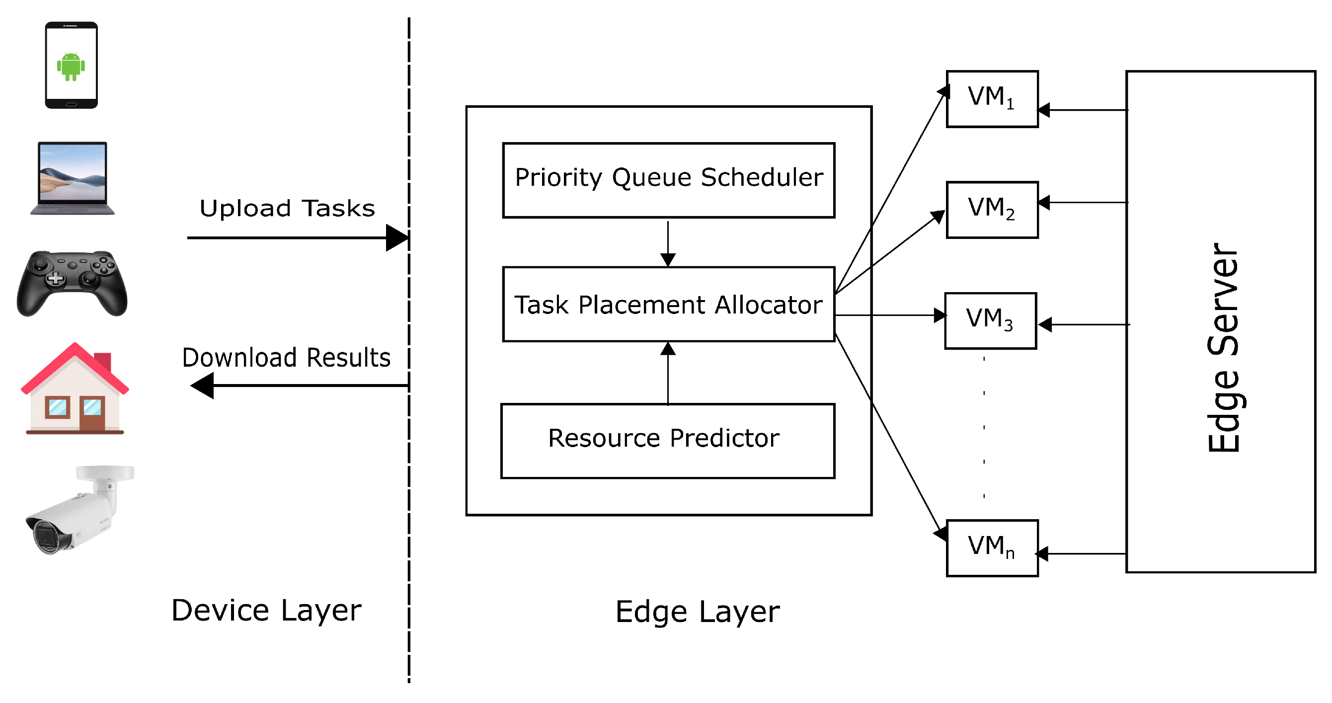
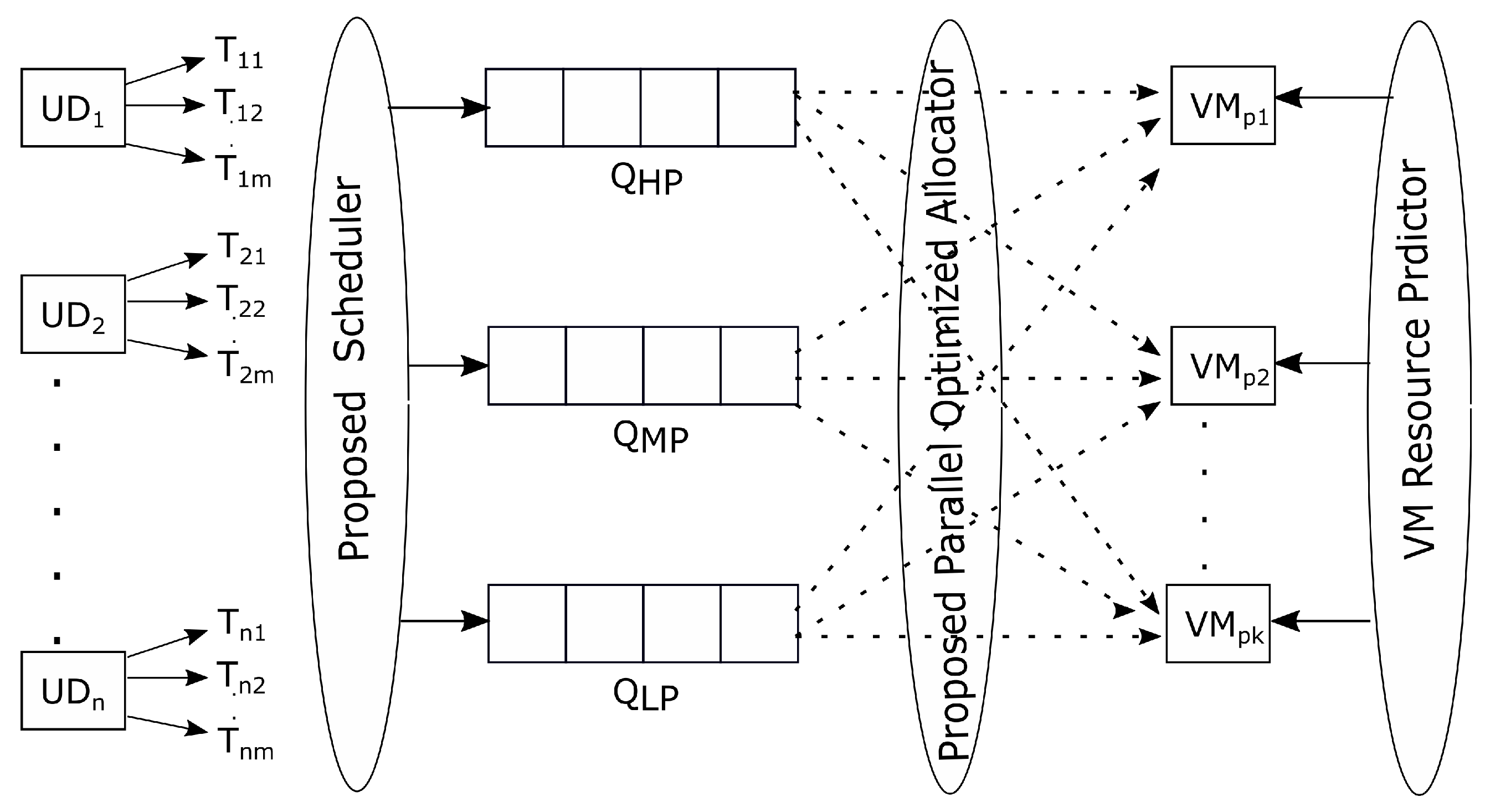
5. Network Architecture

The role of the network architecture is divided into two layers—the device layer and the edge layer. In the device layer, the user devices have uploaded the tasks to the edge server and after computation, the result of the computation is downloaded back to the user device. When the task is reached at the edge layer, the responsibility of the edge layer is divided into three parts—select the suitable priority queue based on the delay sensitivity of the task, predict the available resources, and assign the task to the resource as shown in Figure 1.

When there is a request for task execution in a user device, the first step is to make a suitable decision for finding a suitable place for the computation. Once the decision is chosen for offloading in a suitable MEC for the computation, then the role of the edge layer becomes activated. In the edge layer, the selected offloaded tasks will be placed in a suitable queue scheduler as explained in the DSPS algorithm, given in Algorithm 1. When the task is placed inside the queue, then there will be a requirement to find the suitable VM for the computation, and the suitable VM is predicted with the forecasting of the VM procedure by using the time series analysis.

Algorithm 1: Delay sensitivity-based priority scheduling (DSPS)

The responsibility of the predictor module is divided into two parts. In the first part, we have considered the beginning situation, in which for the first time the VM is predicted by using the Holt-Winters seasonal method, as explained in Algorithm 2, when there is much less historical data available. In the second part, when we have a large dataset, we observed some of the parameters to be dependent on the other parameters for producing a suitable result. Consequently, we used the multivariate vector autoregression (VAR) model to predict the suitable VM as explained in Algorithm 3. We have considered the seasonal methods for the predictions, as we have observed the presence of seasonal patterns while studying similar types of datasets. Once the resource prediction is successfully completed, then the role of the parallel optimized offloader Algorithm 4 becomes active, and the mapping of the task with the most suitable VM lists is predicted by the forecasting procedure, as shown in Figure 2.

Algorithm 2: Holt–Winters-based univariate algorithm (HWVMR)

Algorithm 3: VAR-based multivariate algorithm (VARVMR)

Algorithm 4: Parallel differential evolution-based task allocation (pDETA)

6. Proposed Methodologies

In this section, we discuss the proposed methodologies that consist of a priority scheduler based on the delay sensitivity of the task, univariate and multivariate resource prediction based on time series analysis, and optimized resource utilization based on a parallel differential evolution model.

6.1. Delay Sensitivity-Based Priority Scheduler

When multiple tasks are requested for offloading, then there is a requirement for an optimized scheduling procedure to ensure the smooth execution of the requested tasks by considering the nature of the tasks. Here, we have considered the simplest form of the scheduling procedure by considering [31]. The requested tasks are categorized into three different types based on their sensitivity nature toward the delay. Here, the delay of the task is represented as

$$D{E}_t=D{L}_{SR}-PT.$$

(9)

With the resulting values of the $D{E}_t$, the delay sensitivity is categorized into three types based on the delay scales ranging from (0 to 10), when (1) $D{E}_t$ ranges from 0 to 3, known as higher $D{S}_t$, (2) $D{E}_t$ ranges from 4 to 6, known as medium $D{S}_t$, and (3) $D{E}_t$ ranges from 7 to 10, known as lower $D{S}_t$. $D{S}_t$ is the delay sensitivity of the task, $D{L}_{SR}$ is the service request deadline and PT = current time of the request. Based on the type of delay sensitivity, the type of queue is decided to place the task. When the sensitivity is high, the task needs to be executed with high priority at the beginning, and when the sensitivity is medium, the task needs to be executed with medium priority. Similarly, when the sensitivity is low, it means the task is latency-tolerable in nature, and it needs to be executed with low priority after the completion of the previous two cases, at the end. The task will be placed in a queue based on the threshold values of $T{h}_1$ and $T{h}_2$. The values of the $T{h}_1$ and $T{h}_2$ are set during the experiments. The threshold value of $T{h}_1$ should always be greater than $T{h}_2$. The decision on the suitable queue for the task placement is based on the following conditions:

• $D{S}_t>=T{h}_1$, the task is placed in $Q_{HP}$.
• $D{S}_t<=T{h}_2$, the task is placed in $Q_{LP}$.
• $T{h}_1>D{S}_t>T{h}_2$, the task is placed in $Q_{MP}$.

To ensure a better QoS environment, the total time spent by a service request in the queues should not be greater than the total delay of the task represented below,

$$S{R}_{est}<=D{E}_t,$$

(10)

where $S{R}_{est}$ is the total estimated time of the service request. The DSPS process is represented step-wise in Algorithm 1. This algorithm explains the scheduling of the requested tasks into different priority queues by considering the $D{S}_t,S{R}_{est}$ as inputs. In step 1, when $D{S}_t$ is less than $S{R}_{est}$ and $D{S}_t$ is greater than or equal to $T{h}_1$, it results in step 2 where the task is placed in the $Q_{HP}$. In step 3, when $D{S}_t$ is equal to $S{R}_{est}$ and $D{S}_t$ is greater than $T{h}_2$ and less than $T{h}_1$, then two conditions arise as explained in steps 4 and 7. Step 4 checks whether the $Q_{HP}$ is not full, and then the task is placed in $Q_{HP}$ or otherwise placed in $Q_{MP}$, as given in step 8. Step 13 explains when the $Q_{HP}$ is not full and $D{S}_t$ is less than or equal to $T{h}_2$, then the task is placed in $Q_{MP}$ or else placed in $Q_{LP}$ as given in step 17.

6.2. Time Series-Based VM Resource Predictor

In this section, we discuss the analysis of resource prediction in Section 6.2.1. After the analysis, we explain the process of univariate-based prediction in Section 6.2.2 and multivariate-based prediction in Section 6.2.3. Here, the suitable VM is predicted to provide the best service to the user’s requested task. The main job of this module is to find the best suitable VM from the available list of VMs at a particular time. The prediction module helps in reducing the waiting time of the task so that the ready task will be served very quickly as the suitable VM is ready to serve the state. The reduction in waiting time produced a better result for the delay sensitivity tasks. The next section discusses the prediction analysis process.

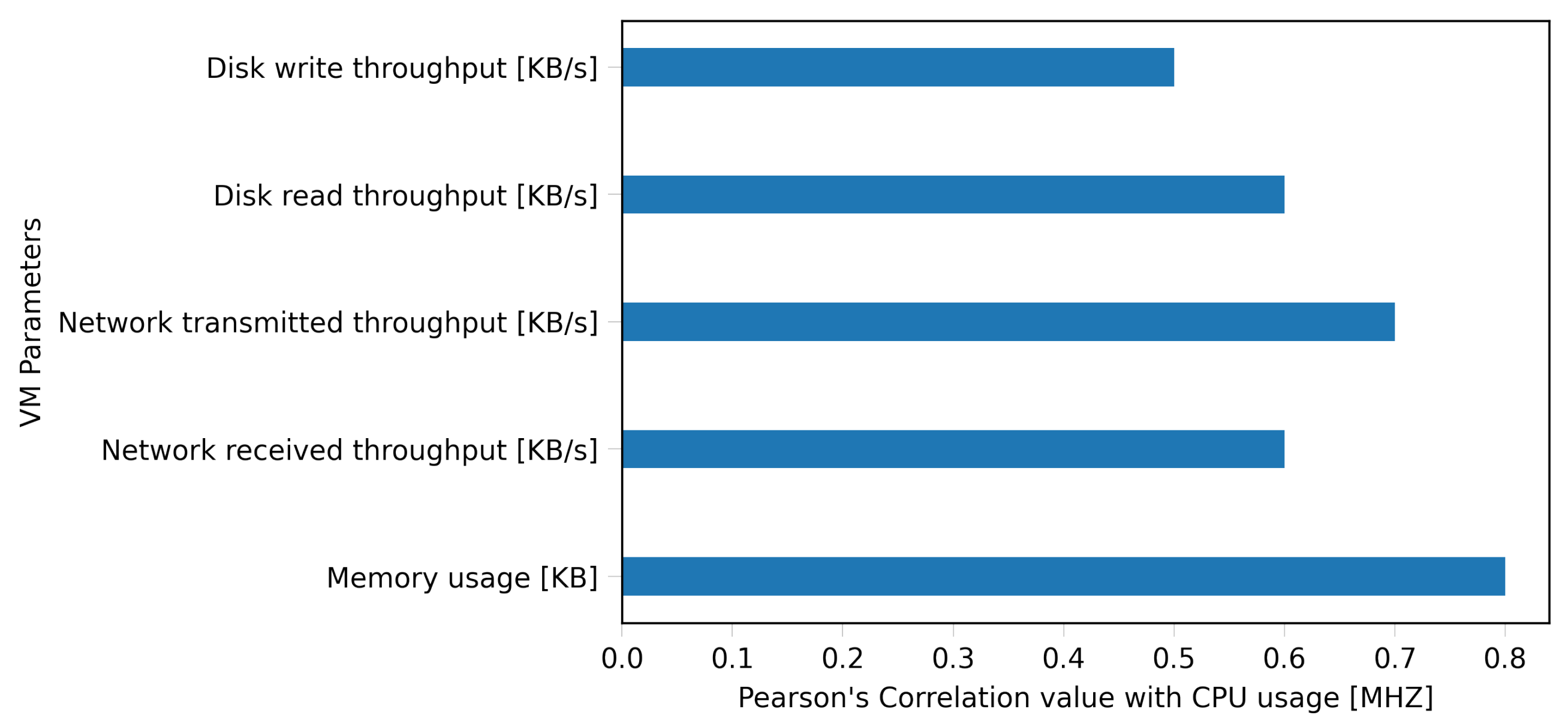
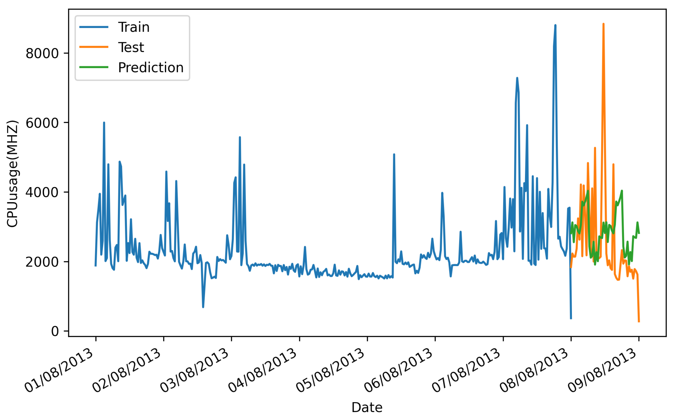
6.2.1. Exploratory Analysis of Resource Prediction

During the thorough review of the different types of predictions [16,21,32,33,34,35,36], we have observed the different types of situations available in the case of the different datasets. Some datasets are univariate (parameters are not dependent on each other) and some are multivariate (parameters are dependent on each other). While observing the seasonal patterns, we found that some of the datasets support seasonal patterns and some are nonseasonal patterns. Consequently, we have concluded that the prediction is fully dependent on the nature of the dataset. As we have used the Bitbrains dataset in our simulation, we found univariate and multivariate seasonal patterns present in the dataset, as shown in Figure 3. Consequently, we have considered the univariate and multivariate seasonal methods to predict the suitable VM.

To deal with the seasonality pattern, we have considered the best suitable Holt–Winters method for prediction, as discussed in Algorithm 2, where considering the task requested by the user, the estimated CPU required is calculated and compared with the available CPU in the VM. The VM is taken from the list of available VMs after predicting the most suitable VM by using the Holt–Winters method.

Based on the dependency among the different parameters to predict the result, we have used the multivariate VAR method for the prediction as explained in Algorithm 3. Once the suitable VM is predicted for a particular task, then the required cost to use the selected VM is calculated by considering the storage cost and computation cost. Here, based on the remaining CPU left, the future service is calculated along with the time required to complete the task successfully.

6.2.2. Applied Holt–Winters-Based Resource Prediction

The Holt–Winters seasonal method is used for forecasting. The forecasting equation comprises three smoothing equations for calculating the level $L_t$, trend $T_t$, and the seasonality $S_t$ with the three smoothing constants as $\alpha ,\beta$, and $\gamma$, as given below,

$$L_t=\alpha \frac{D_t}{S_{t-M}}+(1-\alpha )(L_{t-1}+T_{t-1})$$

(11)

$$T_t=\beta (L_t-L_{t-1})+(1-\beta )T_{t-1}$$

(12)

$$S_t=\gamma \frac{D_t}{L_t}+(1-\gamma )S_{t-M},$$

(13)

where M is calculated by the equation given below:

$$M=\mathit{time period}/\mathit{year}.$$

(14)

The values are M = 4 for quarterly data and M = 12 for yearly data. To forecast the future value $F_{t+1}$ of the required data within the available dataset values we used the Equation (15). To forecast the future value $F_{t+k}$ of the required data within the available dataset values we used the Equation (16). Here, the value of the k is a constant ranging from the $\{1,2,3,\dots \dots ,c\}$. The value of the c depends on the requirement of the future forecast. The constant values of the $\alpha$, $\beta$, and $\gamma$ are set during the experiment:

$$F_{t+1}=(L_t+T_t)S_{t-M+1}$$

(15)

$$F_{t+k}=(L_t+k{T}_t)S_{t-M+k}.$$

(16)

A forecasting error (or residual) is calculated by using the equation given below:

$$Error=F_{t+1}-D_{t+1}.$$

(17)

In Algorithm 2, while considering the task requested by the user, the estimated $CPU\_required$ is calculated and compared with the $CPU\_available$ in the VM, from the list of available VMs to predict the most suitable VM by using the Holt–Winters method.

6.2.3. Applied VAR Based Resource Prediction

This is a type of forecasting method, where the present forecasting is calculated based on the previous past value. Here, the forecasting of the resource at the present time t; $F_t$ depends on the product of the past value of the resource (i.e., $F_{t-1}$ with the corresponding coefficients and C is added with the error term $E_t$, as shown in the equation given below):

$$F_t=C{F}_{t-1}+{ϵ}_t.$$

(18)

In this paper, we have calculated the forecasting of the $CPU\_usage\left(X_t\right)$ and $Memory\_usage\left(Y_t\right)$ by using the Equation (19) and Equation (20), where $X_t$ is calculated by using the coefficients $C_{11}$ and $C_{12}$ by multiplying with the previous value of the $X_t$, i.e., $X_{t-1}$, which is added with the corresponding error term. Here, $Y_t$ is calculated in a similar way. Equation (21) is a general vector representation of the forecasting of resources. We have

$$X_t=C_{11}{X}_{t-1}+C_{12}{X}_{t-1}+{ϵ}_{t1}$$

(19)

$$Y_t=C_{21}{Y}_{t-1}+C_{22}{Y}_{t-1}+{ϵ}_{t2}$$

(20)

$$\left[\begin{array}{c}{X}_t\\ Y_t\end{array}\right]=\left[\begin{array}{cc}{C}_{11}& C_{12}\\ C_{21}& C_{22}\end{array}\right]\left[\begin{array}{c}{X}_{t-1}\\ Y_{t-1}\end{array}\right]+\left[\begin{array}{c}{ϵ}_{t1}\\ {ϵ}_{t2}\end{array}\right],$$

(21)

where $X_t$ and $Y_t$ are the forecasting variables at time t. $C_{11}$, $C_{12}$, $C_{21}$ and $C_{22}$ are the corresponding coefficients. $X_{t-1}$ and $Y_{t-1}$ are the past values of the $X_t$ and $Y_t$, respectively. ${ϵ}_{t1}$ and ${ϵ}_{t2}$ are the error terms.

During the analysis of the dataset, we found some dependencies among the different parameters while applying Pearson’s correlation. Figure 4 shows the correlation analysis result. As the Pearson coefficient of memory usage is high with respect to CPU usage, we have considered the CPU usage and memory usage parameter for the prediction. Figure 5 shows the behaviour of the actual CPU usage and Figure 6 shows the behaviour of the actual memory usage. Based on the observed dependency, we have applied VAR model to generate the behaviour of the actual CPU usage versus the prediction as shown in Figure 7 and the actual memory usage versus the prediction as shown in Figure 8.

In Algorithm 3, we have predicted the capacity of the VM and calculated the execution cost (C) and the total time (t) taken by the input task during the process, by considering the set of tasks $\{T_1,T_2,\dots \dots ,T_n\}$ as inputs. In step 1, we have initialized all the variables as t, C, and $wait\_time$ as 0. In step 2, a loop is used for a single task in the set of tasks calculating the desired results. In step 4, for each VM in the set of VM lists $\{V{M}_1,V{M}_2,\dots ,V{M}_m\}$, we find that after checking the condition, the $CPU\_required$ is less than the $CPU\_capacity$ in step 3. Step 5 is used to predict the VM by using the multivariate VAR method by using Equations (19) and (20). Once the suitable VM is predicted for a particular task, then the required cost to use the selected VM is calculated by considering the storage cost and computation cost in step 6. In step 7, the CPU capacity of the VM is assigned to the CPU available for the computation of the task. CPU required for the computation of the task is assigned to the $CPU\_assigned$ in step 8. Step 9 is used for calculating the remaining CPU left out in the VM resource for the future service, after assigning the task by subtracting the $CPU\_assigned$ from the $CPU\_available$ by the VM resource. When the suitable VM is predicted for the task, the total time required to complete the process is calculated in step 11, by the addition of the previously calculated time and the waiting time.

6.3. Parallel Optimal Allocator

In this section, we discuss the finding of a suitable VM in Section 6.3.1 and then assign the requested task to the suitable VM by applying the parallel differential evolution algorithm as explained in Section 6.3.2 (Figure 9, Figure 10 and Figure 11). Once the forecasting of the available VM resources is listed successfully, the next part is to find the suitable VM for the mapping with the requested task. The suitable VM is found by using the Algorithm 4. Here, we first find the suitable VMs by using Equation (22), and then we sort all the VMs in ascending order of their distances. Then, for each requested task, with sufficient availability of the CPU and memory capacity, the suitable VM is chosen by the parallel differential evolution Algorithm 4 as explained in Section 6.3.2. Then, the placement of the requested task with the most suitable VM is executed.

6.3.1. Finding Suitable VM by Using Minkowski Distance

To find the suitable VM for task assignment, the deviation between the resource availability in VMs and the resource required by the task is computed by using the Minkowski distance as given in Equation (22). The suitable VM is selected where the deviation is minimum. In Equation (22), the value of p is an integer. The equation behaves differently when the value of the p is changed. If p = 1, it is considered as a Manhattan distance, and if p = 2, it is considered as a Euclidean distance. Consequently, depending on the demand of the requirement we can consider the value of p as 1 or 2. The p value will be 1 when the dimension in the data will become very high. In this work, we have considered the value of p as 2, which is similar to the Euclidean distance. We have

$$Distance={\left(\sum _{i=1}^n{\left|R_i[CPU,Mem]-r_i[CPU,Mem]\right|}^p\right)}^{1/p}.$$

(22)

6.3.2. Parallel Differential Evolution Algorithm

Edge servers have limited resources, so the possible numbers of VMs are fewer compared with the cloud servers. One solution for getting a faster computation result is by making the process parallel. The parallel differential evolution algorithm helps to optimize parallel computation with limited resources in less time with the mutation, crossover, and selection procedure of the differential evolution algorithm shown in Figure 9. We select the suitable task placement with the available predicted VMs in a much faster and easier way than the other machine learning algorithms by using the parallel differential evolution process as shown in Figure 11.

To apply the differential evolution algorithm in our procedure, we need to set the following parameters.

• Problem definition: Our aim is to assign the task to a suitable predicted VM from the predicted VM lists with the optimum allocation of resources considering minimum distance by applying Equation (22). The mapping of the available VM resources with the required task resources. Here, the resources are CPU usage and memory usage for the VMs and tasks. The task is assigned to the VM only when the following equation will be satisfied:

  $$R_i[CPU,Mem]>r_i[CPU,Mem].$$

  (23)
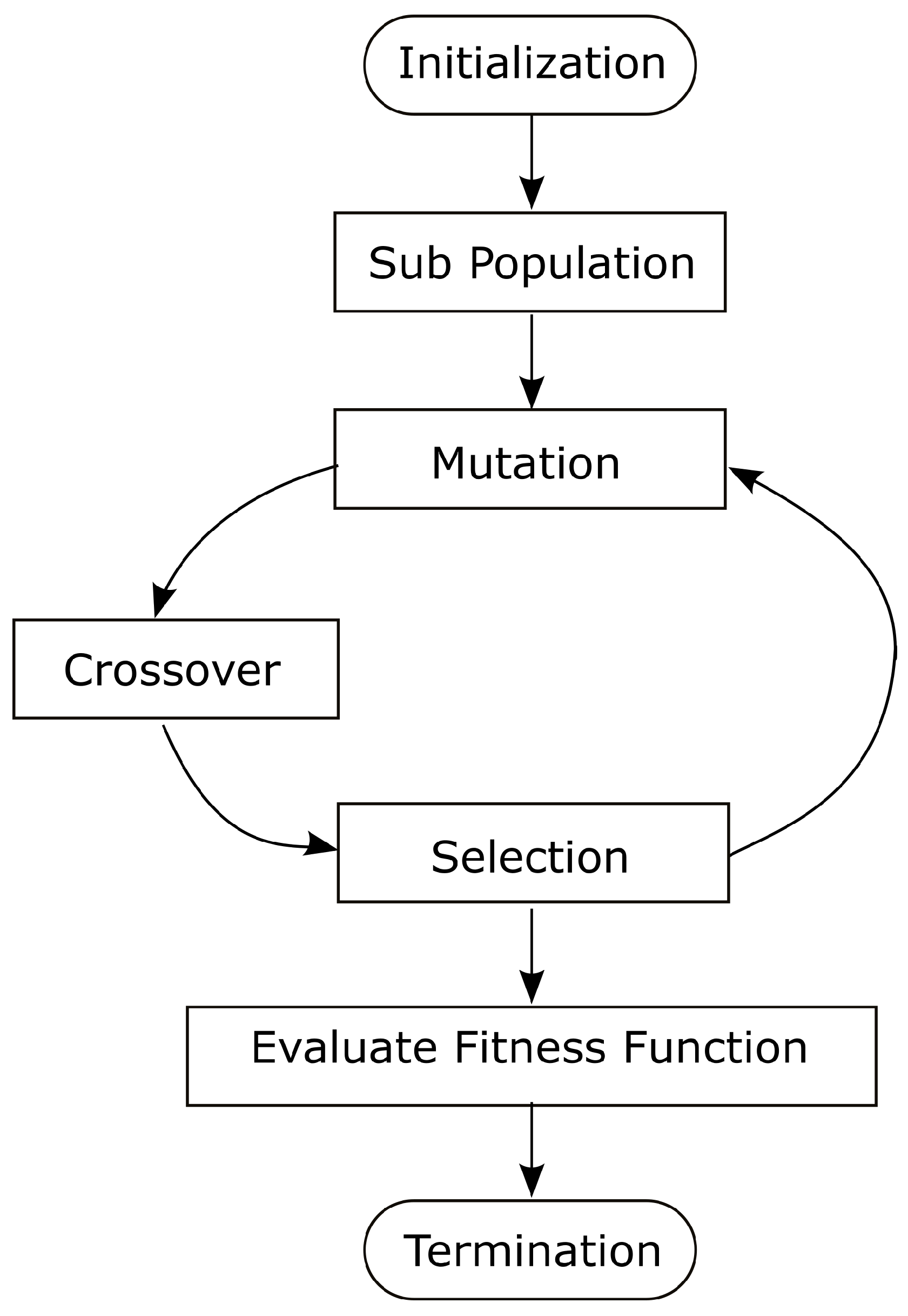
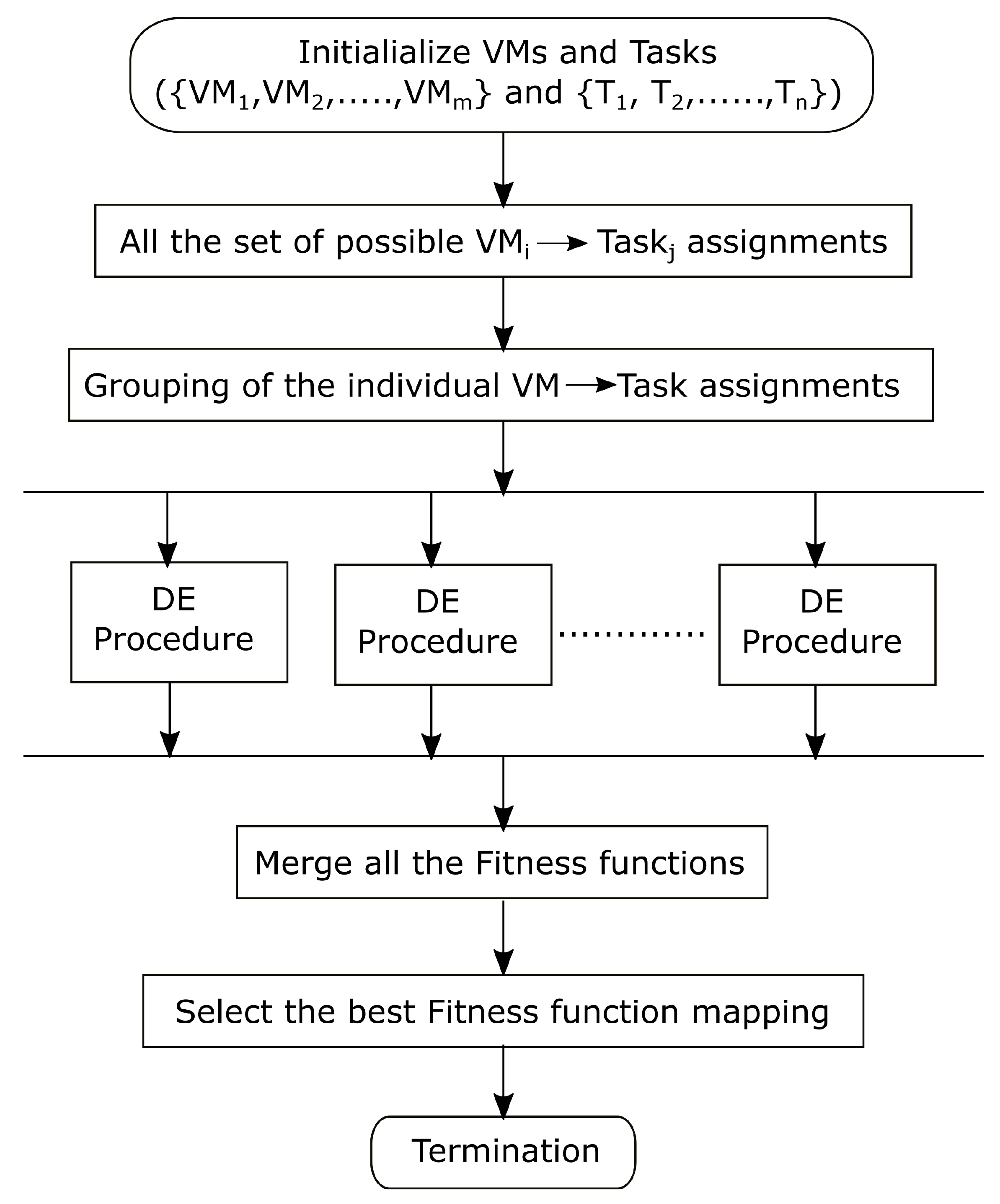
• Problem parameters: The population size (N) is $P_s$, the dimension of the problem (D) is 4, the stopping criteria (maximum number of iterations) is set to 5, the scaling factor (F) is 0.5, and the crossover probability $P_{cr}$ is 0.7. The value of the scaling factor is inversely proportional to the local search ability, so we have considered a minimum value for the scaling factor, i.e., 0.5 to become strong in the local search algorithm.

  Figure 9. Differential evolution procedure.

  Figure 9. Differential evolution procedure.
• Initialization: Based on $P_s$, the number of initial solutions are obtained by satisfying the problem definition. Here, all the possible assignments take place and discover the best solution having minimum result by applying Equation (22).
• Differential evolution position update: Here we have considered the suitable strategy as DE/Best/1/2 for binomial crossover based on two randomly assigned pairs. The generations are formed based on the above procedure. Here, we have discussed the process followed in one generation.
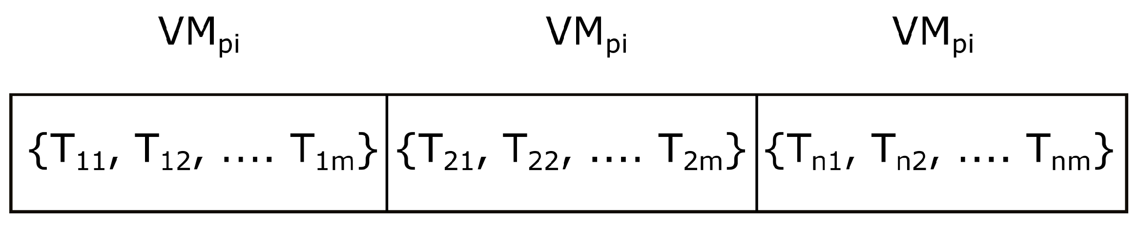
• Chromosome formation: In the beginning, we assign the predicted VM resources from the set of $\{V{M}_{p1}$, $V{M}_{p2}$, ……, $V{M}_{pm}\}$ with the set of requested tasks $\{T_{11},T_{21},\dots \dots ,$$T_{nm}\}$ available in the priority scheduled queues. The active tasks will become 1, and the inactive tasks will become 0 in the different task sets present in the chromosome. The chromosome is represented in Figure 10.

  Figure 10. Representation of chromosome.

  Figure 10. Representation of chromosome.
• Population: We collect all the chromosomes, and make them ready for the parallel computation of the individual population by using the differential evolution algorithm.
• Subpopulation: We consider a single population for finding the fitness function until the termination condition arrives. Here, the subpopulations are implemented in parallel to finding the fitness function for an individual one.
• Fitness function: This refers to the calculation of the computation time, cost, and energy required for the computation in edge resources.
  The best fitness function = {$Min\left(C_t\left(i\right)\right)$, $Min\left(C_T\left(i\right)\right)$, $Min\left(E_t\left(i\right)\right)$}.
• Mutation: The predicted VM resource is assigned with the possible set of requested tasks from the priority scheduled queues. The output of the mutation module is the input to the crossover module. Once the single output is released to the crossover module for the individual assignment, the mutation module is ready with the next possible assignment of the task to the VM resource. The best suitable mutation strategy is the “DE/Best/1/2” as

  $$V^{\mu G}=X_{best}^{\mu G}+F(X_{r1}^{\mu G}-X_{r2}^{\mu G}),$$

  (24)

  where $X_{best}^{\mu G}$ is the best solution produced during the initialization process, $X_{r1}^{\mu G}$ and $X_{r2}^{\mu G}$ are the random solutions selected from the population, and $X_{r1}^{\mu G}\ne X_{r2}^{\mu G}$, F is a scaling factor, and $V^{\mu G}$ is mutant donor vector.
• Crossover: The crossover method increases the diversity of the population. This module is ready for the calculation of the fitness function for the input to the mutation module. The crossover method is shown below,

  $$U_i^c=\left\{\begin{array}{c}{V}_i^{c}ifr\le C_{p}ori=\delta \hfill \\ X_i^{c}ifr>C_{p}andi\ne \delta \hfill \end{array}\right.,$$

  (25)

  where $U_i^c$ is the ith variable of the trial vector, $V_i^c$ is the ith variable of the donor vector, $X_i^c$ is the ith variable of the target vector, r is the random number between 0 and 1, $C_p$ is the crossover probability, $\delta$ is the randomly selected variable location, and $\delta$ $ϵ$ {1, 2, 3, …, D}.
• Selection: This module selects the best mapping of the predicted VM resource with the requested task by applying Equation (22). It takes the output of the crossover module and finds the best fitness function for the selection of the task placement of the individual subpopulation.
• Termination: The termination condition arrives when we obtained the best fitness function with the minimum computation time, cost, and energy after merging all the fitness functions calculated from the individual subpopulations. After the termination condition was reached, we obtained the optimized placement of the requested task in the VM.

The whole process of parallel differential evolution is expressed in Algorithm 4, which explains the mapping of the tasks (available in the priority queues; $Q_{HP},Q_{MP}$, and $Q_{LP}$) into the selected predicted $VM$ lists {$V{M}_{p1}$, $V{M}_{p2}$, …, $V{M}_{pm}$}. The tasks are the outputs of Algorithm 1, and the predicted VMs are the outputs from Algorithm 2 or Algorithm 3 based on the nature of the dependencies of the different available parameters of the dataset. Considering a particular time period from the predicted list of $VMs$ of step 1 and step 2, we learn the suitable $VM$ resources by using the Minkowski distance, as explained in Equation (22). All the suitable VMs are stored in a list in step 3. In step 4, we perform the sorting in ascending order of the suitable $VM$ from the $S_N$ list and assigned it to the new list $S_A$. In step 7, we make the population by randomly assigning $VM$ from the list of $S_A$ to the available task set T. In step 8, for each available chromosome $ch$ from the population P, we assign the task to the suitable $VM$ from the sorted list $V{M}_s$. For each suitable $VM$ from the chromosome in step 9, we choose the task k from the task set in step 10 by checking whether the CPU capacity of the $VM$ should be greater than the CPU required by the requested task in step 11. Similarly, we check if the memory capacity of the $VM$ resources should be greater than the memory required by the requested task in step 12. When both conditions are satisfied, then we have added the task to the task set of assigned $V{M}_s$ in step 13. In step 19, we make a set of subpopulations by selecting chromosomes randomly from the population P. To make all the executions parallel, we select v (taken as 50) as the number of subpopulations at a time for computing steps 21 to 24. For each subpopulation, the mutation is done in step 21 and assigned to M; in step 22, we perform the corresponding crossover and assign it to C. The fitness function is calculated based on the execution time, cost, and energy in step 23. The suitable selection is assigned to S in step 24. In step 26, the best fitness value is assigned to the variable Place. We assign the chromosome of the variable Place to variable $ch$ in step 27, and finally, the best-fitting chromosome having the suitable $VM$ with the task assignment is returned in step 28.

Figure 11. Parallel differential evolution process.

Figure 11. Parallel differential evolution process.

7. Simulation Results

In this section, our proposed approach is simulated, and the benefits of computation offloading processes in the MEC environment are justified. The proposed method is evaluated by using the average waiting time, scheduled task, makespan(s), load-balancing level, and different types of time series analysis, cost, and energy with respect to the number of service requests, tasks, and VMs. For performance verification, our method is compared with the RR, priority, GAF [24], min–min, DE, and MTSS [25] algorithms. The simulation is performed by using Python 3.8 with 4 GB RAM, and an i5 processor in Windows 8 environment. The proposed Algorithm 4 is implemented by using the multithreading class ThreadPoolExecutor of concurrent.futures module in Python to achieve parallelism. The simulation setup uses the simulation parameters available in

Table 1. Simulation parameters.

Parameter	Value
Number of tasks	50 to 600
Size of the task	2 to 20 GI
Number of VMs	5 to 30
VM processing speed	10 GIPS
Latency–sensitivity	0 to 10

.

Figure 12 shows the average waiting time of the tasks based on the number of service requests arrived. Here, the RR scheduling algorithm consumes maximum waiting time as they followed the time slice quantum rules, where a larger task fails to meet the requirements as it consumes maximum time quantum to finish its request. In priority scheduling, the highest-priority task takes more attention, due to which the lowest-priority tasks suffer and result in the maximum waiting time to fulfill the service request. In GAF scheduling, they have set a baseline based on the largest deadline received, which becomes inactive in a random environment when a larger deadline task arrives later after setting the baseline, but this scheduling performs better than the above two until the larger deadline of the task is not changed in the future. Our proposed scheduling algorithm performs better than the RR, priority, and GAF, as it combines the best features of the priority and RR scheduling by considering the latency sensitivity of the tasks.

Figure 13 shows the task scheduling performance based on the number of service requests. When there is a lesser number of tasks, limited to 60 numbers of tasks, then all the scheduling algorithms perform almost similarly. The difference in scheduling tasks arises when the tasks are more than 60 in number. Our proposed algorithm outperforms other scheduling algorithms. Our approach results in 98% of the tasks being scheduled with minimum processing time, as our scheme is based on priority and RR scheduling. GAF also performs better than the priority and RR algorithms, as it considers the largest deadline task at the end. As we are getting the set of tasks with a mixture of different priorities, so by experimenting with the different set of percentages, we have fixed the percentage as 70% from the high-priority queue, 20% from the medium-priority queue, and 10% from the low-priority queue; as a result, we will always get the set of ready tasks with a mixed type, which results in all the tasks being easily scheduled with minimum waiting time and able to overcome the starvation problem.

We have considered Holt–Winters time series method to predict future VM resources. We have used the GWA-T-12 Bitbrains dataset [17] for our implementation. By using the additive decomposition model, we have found the graph as shown in Figure 3. The graph is divided into four different parts. The first part describes the general representation of the actual time series data of CPU usage, the second part describes the trend patterns available in the dataset, the third part describes the changes in the seasonal components, and the fourth part describes the residual errors available in the prediction of the CPU usages. Figure 14 shows the CPU usage plots, where the blue colour represents the training dataset and the orange colour represents the testing of the dataset. Here, the training and testing of the dataset are in the ratio of 90:10. Figure 15 shows the train and test data with the future prediction of CPU usage. Here, we have obtained 35.17% of the mean absolute percentage error.

Figure 16 shows a faster task-completion time than the other algorithms while the number of tasks is increasing further. Here, we have assumed the situation in which the performance of the task-completion time observes while increasing the number of tasks in a constant VM environment. The task-completion time increases when the number of tasks increases. The DE performs better than the min–min algorithm with the optimization strategy and MTSS performs better than the DE with the advanced and improved DE strategy. Our proposed approach performs better than the MTSS with the improved and parallel DE algorithm. The parallel DE helps in the improvement by 18.95%, 26.46%, and 34.43% with the approaches MTSS, DE, and min–min respectively.

Figure 17 shows the task-completion time based on the number of VMs available in the MEC environment. Here, we have considered 100 scheduled tasks. The task-completion time results in better performance when the available resources are greater, representing that the task-completion time is inversely proportional to the number of VMs. Here, the MTSS algorithm performs better than the conventional DE and min–min algorithm, as it has considered the improved version of DE. However, our proposed approach improves the performance by 18.95%, 26.46%, and 34.43% with the approaches MTSS, DE, and min–min respectively, due to the applied parallel computation in the improved DE algorithm.

The resource utilization of VM is measured by using the workload-balancing level. Figure 18 shows the changes in the load-balancing level with the increasing number of tasks. When the number of tasks increases, the load-balancing level gradually becomes difficult as the number of VMs is constant. Here the min–min algorithm does not perform well, as it considers only the execution time of the task. The DE algorithm performs better than the min–min as it considers the global optimization-based algorithm. The MTSS algorithm performs better than the DE and min–min as it considers the “Q-value method” in its algorithm. Our proposed approach performs better than the other three algorithms, as it uses the parallel DE algorithm, due to which the waiting time for the tasks also decreases to a greater extent. The workload balance factor improved by 28.78%, 38.58%, and 62.87% with the approaches MTSS, DE, and min–min respectively.

Figure 19 shows the change in the cost of execution of the task based on the increasing number of tasks. Here the cost increases with an increase in the number of tasks. The min–min algorithm shows the worst performance when compared with the other algorithms, as it uses the high-performance VM for task computation. Our proposed approach shows better performance than the other algorithms, as it uses the most suitable VM for the execution of the task. For choosing the suitable VM, we first checked the capacity of the available resources of the VM, and based on the availability, the delay sensitivity of the task has been assigned to the predicted VM. This process minimizes the waiting time, which results in a decrease in the cost of the execution by 22.41%, 35.35%, and 68.63% with the approaches MTSS, DE, and min–min, respectively.

Figure 20 shows the energy consumption by the edge server with the increase in the number of tasks. The min–min algorithm shows the worst performance when compared with the other algorithms, as it uses the high-performance VM for task computation. Our proposed approach shows better performance than the other algorithms as it uses the nearby most suitable VM for the execution of the task. By considering the effective resource utilization of the edge server, the delay sensitivity task has been assigned to the nearby predicted VM. This process minimizes the energy consumption, which results in the decrease in energy of the computation by 40.78%, 51.76%, and 77.68% with the approaches MTSS, DE, and min–min, respectively.

8. Conclusions and Future Work

Task offloading of resource-hungry applications and edge VM resource allocation has been a thrust area of focus due to its vast applications in the 5G/6G-enabled MEC environment. In this paper, edge server-side issues are considered once the tasks are decided to be offloaded, and we propose a DSPS policy to schedule the tasks as per their deadline. Furthermore, exploratory data analysis is carried out, and inference has been made regarding seasonal patterns in the usage of edge CPU resources from the GWA-T-12 Bitbrains VM utilization dataset. Based on the analysis, the availability of VM resources of the edge server is predicted by using the HWVMR and VARVMR algorithms. Finally, for optimal and fast task assignment, the pDETA algorithm is proposed. The proposed algorithms are compared with some state-of-the-art algorithms like MTSS, traditional DE, and min–min, and the performance evaluations measure the cost and energy matrix. The improvements observed are 22%, 35%, and 69% for cost and 41%, 52%, and 78% for energy, respectively. In the future, different optimization techniques can be used to optimize the performance of the algorithm, and this algorithm can be analyzed in a heterogeneous and multiuser environment. Further, mobility-based task allocation and orchestration can be integrated considering multiple server scenarios.

References

1. Abdullah, A.; Ibrahim, E.; Muthanna, A.; Alghamdi, A.; Mohammed, A.; Adel, A. Efficient multi-player computation offloading for VR edge-cloud computing systems. Appl. Sci. 2020, 10, 5515. [Google Scholar]
2. Kai, P.; Peichen, L.; Tao, H. A privacy-aware computation offloading method for virtual reality application. CEUR Workshop Proc. 2021, 3052. [Google Scholar]
3. Ke, Z.; Yuming, M.; Supeng, L.; Quanxin, Z.; Longjiang, L.; Xin, P.; Li, P.; Sabita, M.; Yan, Z. Energy-efficient offloading for mobile edge computing in 5g heterogeneous networks. IEEE Access 2016, 4, 5896–5907. [Google Scholar]
4. Jinke, R.; Guanding, Y.; Yunlong, C.; Yinghui, H. Latency optimization for resource allocation in mobile-edge computation offloading. IEEE Trans. Wirel. Commun. 2018, 17, 5506–5519. [Google Scholar]
5. Mian, G.; Mithun, M.; Gen, L.; Jinyou, Z. Computation offloading for machine learning in industrial environments. In Proceedings of the IECON 2020 The 46th Annual Conference of the IEEE Industrial Electronics Society, Singapore, 18–21 October 2020; pp. 4465–4470. [Google Scholar]
6. Juan, F.; Jiamei, S.; Shuaibing, L.; Mengyuan, Z.; Zhiyuan, Y. An efficient computation offloading strategy with mobile edge computing for IoT. Micromachines 2021, 12, 204. [Google Scholar]
7. Sharma, V.; Rai, V.P.; Sharma, K.K. Edge computing: Needs, concerns and challenges. Int. J. Sci. Eng. Res. 2017, 8, 154–166. [Google Scholar]
8. Junaid, Q.; Beatriz, S.-D.-A.; Anwar, K.; Begoña, G.-Z.; Isabel, D.L.T.-D.; Hasan, M. Towards mobile edge computing: Taxonomy, challenges, applications and future realms. IEEE Access 2020, 8, 189129–189162. [Google Scholar]
9. Huaming, W.; William, K.; Katinka, W. An efficient application partitioning algorithm in mobile environments. IEEE Trans. Parallel Distrib. Syst. 2019, 30, 1464–1480. [Google Scholar]
10. Delowar, H.M.; Tangina, S.; Alamgir, H.M.; Imtiaz, H.M.; Junyoung, H.L.N.P.; Nam, H.E. Fuzzy decision-based efficient task offloading management scheme in multi-tier MEC-enabled networks. Sensors 2021, 21, 1–26. [Google Scholar]
11. Jiuyun, X.; Zhuangyuan, H.; Xiaoting, S. Optimal offloading decision strategies and their influence analysis of mobile edge computing. Sensors 2019, 19, 3231. [Google Scholar]
12. Jun, C.; Dejun, G. Research on task-offloading decision mechanism in mo- bile edge computing-based internet of vehicle. Eurasip J. Wirel. Commun. Netw. 2021, 2021, 1–14. [Google Scholar]
13. Changsheng, Y.; Kaibin, H.; Hyukjin, C.; Byoung-Hoon, K. Energy-efficient resource allocation for mobile-edge computation offloading. IEEE Trans. Wirel. Commun. 2017, 16, 1397–1411. [Google Scholar]
14. Xihan, C.; Yunlong, C.; Liyan, L.; Minjian, Z.; Benoit, C.; Lajos, H. Energy-efficient resource allocation for latency-sensitive mobile edge computing. IEEE Trans. Veh. Technol. 2020, 69, 2246–2262. [Google Scholar]
15. Jiadai, W.; Lei, Z.; Jiajia, L.; Nei, K. Smart resource allocation for mobile edge computing: A deep reinforcement learning approach. IEEE Trans. Emerg. Top. Comput. 2021, 9, 1529–1541. [Google Scholar]
16. Deng, X.; Li, J.; Liu, E.; Zhang, H. Task allocation algorithm and optimization model on edge collaboration. J. Syst. Archit. 2020, 110, 1–12. [Google Scholar] [CrossRef]
17. The Grid Workloads Gwa-t-12 Bitbrains. Available online: http://gwa.ewi.tudelft.nl/datasets (accessed on 27 September 2022).
18. Zeyi, T.; Qi, X.; Zijiang, H.; Cheng, L.; Lele, M.; Shanhe, Y.; Qun, L. A survey of virtual machine management in edge computing. Proc. IEEE 2019, 107, 1482–1499. [Google Scholar]
19. Sun, L.; Li, Z.; Lv, J.; Wang, C.; Wang, Y.; Chen, L.; He, D. Edge computing task scheduling strategy based on load balancing. MATEC Web Conf. 2020, 309, 3025. [Google Scholar] [CrossRef] [Green Version]
20. Hansun, S.; Charles, V.; Indrati, C.R.; Saleh, S.S. Revisiting the holt-winters’ additive method for better forecasting. Int. J. Enterp. Inf. Syst. 2019, 15, 43–57. [Google Scholar] [CrossRef]
21. Shahin, A.A. Using Multiple Seasonal Holt-Winters Exponential Smoothing to Predict Cloud Resource Provisioning. Int. J. Adv. Comput. Sci. Appl. 2016, 7, 91–96. [Google Scholar]
22. Sarikaa, S.; Niranjana, S.; Deepika, K.S.V. Time Series Forecasting of Cloud Resource Usage. In Proceedings of the 2021 IEEE 6th International Conference on Computing, Communication and Automation (ICCCA), Arad, Romania, 17–19 December 2021; pp. 372–382. [Google Scholar]
23. Ouhame, S.; Hadi, Y. Multivariate workload prediction using Vector Autoregressive and Stacked LSTM models. In Proceedings of the ACM SMC Conference (SMC’19), ACM, Kenitra, Morocco, 28–29 March 2019; pp. 1–7. [Google Scholar]
24. Tseng, C.W.; Tseng, F.H.; Yang, Y.T.; Liu, C.C.; Chou, L.D. Task Scheduling for Edge Computing with Agile VNFs On-Demand Service Model toward 5G and beyond. Wirel. Commun. Mob. Comput. 2018, 2018, 1–13. [Google Scholar] [CrossRef] [Green Version]
25. Zhou, Z.; Li, F.; Yang, S. A Novel Resource Optimization Algorithm Based on Clustering and Improved Differential Evolution Strategy under a Cloud Environment. ACM Trans. Asian Low-Resour. Lang. Inf. Process. 2021, 20, 5. [Google Scholar] [CrossRef]
26. Sardaraz, M.; Tahir, M. A parallel multi-objective genetic algorithm for scheduling scientific workflows in cloud computing. Int. J. Distrib. Sens. Netw. 2020, 16, 8. [Google Scholar] [CrossRef]
27. Skorpil, V.; Oujezsky, V. Parallel genetic algorithms’ implementation using a scalable concurrent operation in python. Sensors 2022, 22, 2389. [Google Scholar] [CrossRef]
28. Laili, Y.; Guo, F.; Ren, L.; Li, X.; Li, Y.; Zhang, L. Parallel scheduling of large-scale tasks for industrial cloud-edge collaboration. IEEE Internet Things J. 2021, 4662, 1–13. [Google Scholar] [CrossRef]
29. Sun, Y.; Song, C.; Yu, S.; Liu, Y.; Pan, H.; Zeng, P. Energy-efficient task offloading based on differential evolution in edge computing system with energy harvesting. IEEE Access 2021, 9, 16383–16391. [Google Scholar] [CrossRef]
30. Li, X.; Zeng, F.; Fang, G.; Huang, Y.; Tao, X. Load balancing edge server placement method with QoS requirements in wireless metropolitan area networks. IET Commun. 2020, 14, 3907–3916. [Google Scholar] [CrossRef]
31. Guruprasad, H.S.; Dakshayini, M. An optimal model for priority based service scheduling policy for cloud computing environment. Int. J. Comput. Appl. 2011, 32, 975–8887. [Google Scholar]
32. Tu, Y.; Chen, H.; Yan, L.; Zhou, X. Task offloading based on LSTM prediction and deep reinforcement learning for efficient edge computing in IoT. Future Internet 2022, 14, 30. [Google Scholar] [CrossRef]
33. Rob, H.J.; Anne, K.B.; Ralph, S.D.; Simone, G. A state space framework for automatic forecasting using exponential smoothing methods. Int. J. Forecast. 2002, 18, 439–454. [Google Scholar]
34. Prieto, O.J.; Alonso-González, C.J.; Rodríguez, J.J. Stacking for multivariate time series classification. Pattern Anal. Appl. 2015, 18, 297–312. [Google Scholar] [CrossRef]
35. Dissanayake, B.; Hemachandra, O.; Lakshitha, N.; Haputhanthri, D.; Wijayasiri, A. A comparison of ARIMAX, VAR and LSTM on multivariate short-term traffic volume forecasting. In Proceedings of the 2021 28th Conference of Open Innovations Association, Moscow, Russia, 27–29 January 2021; pp. 564–570. [Google Scholar]
36. Zoltan, B.; Laszlo, D.; Janos, A. Dynamic principal component analysis in multivariate time-series segmentation. Conserv. Inf. Evol. 2011, 1, 11–24. [Google Scholar]
Figure 1. MEC network architecture.
Processes 11 01017 g001
Figure 2. Proposed task-execution process.
Processes 11 01017 g002
Figure 3. Analysis of trend and seasonal components of CPU usage.
Processes 11 01017 g003
Figure 4. Pearson’s correlation of CPU usage with other VM parameters.
Processes 11 01017 g004
Figure 5. Behaviour of actual CPU usage.
Processes 11 01017 g005
Figure 6. Behaviour of actual memory usage.
Processes 11 01017 g006
Figure 7. Behaviour of actual CPU usage and prediction result.
Processes 11 01017 g007
Figure 8. Behaviour of actual memory usage and prediction result.
Processes 11 01017 g008
Figure 12. Performance evaluation by using average waiting time with the number of service requests.
Processes 11 01017 g012
Figure 13. Performance evaluation by using number of service requests with the scheduled tasks.
Processes 11 01017 g013
Figure 14. Training and testing result of the CPU usage.
Processes 11 01017 g014
Figure 15. Prediction of CPU usage by using Holt–Winters method.
Processes 11 01017 g015
Figure 16. Performance evaluation by using task completion time with the number of tasks.
Processes 11 01017 g016
Figure 17. Performance evaluation by using task-completion time with the number of VMs.
Processes 11 01017 g017
Figure 18. Performance evaluation by using load balancing with number of tasks.
Processes 11 01017 g018
Figure 19. Performance evaluation of cost with number of tasks.
Processes 11 01017 g019
Figure 20. Performance evaluation of average energy with a number of tasks.
Processes 11 01017 g020