3.2.3. Gas–Solid Chemical Reaction Model
The chemical reactions of raw material particles occur in the furnace under sulfur gas reduction. Hence, the turbulent chemical reaction model was chosen as a generic finite rate model, i.e., the mass fraction of each substance was predicted by solving the component conservation equations of the chemical substances [
29]. The generalized form of the conservation equation is expressed as follows:
where
Yt is the mass fraction of substance i,
Rt is the net rate of the chemical reaction production, and
St is the additional rate of production in the discrete phase. If there are N substances in the system, the N-1 equations must be solved. The sum of the mass fractions of N substances is 1, and the mass fraction of the Nth substance is obtained by subtraction. Hence, the Nth substance must be the one with the largest mass fraction to minimize the numerical error. The interaction of turbulent chemical reactions is modeled using the vortex dissipation conceptual model, which allows the careful Arrhenius chemical kinetics to merge in turbulence, thereby simultaneously increasing the computational cost [
30].
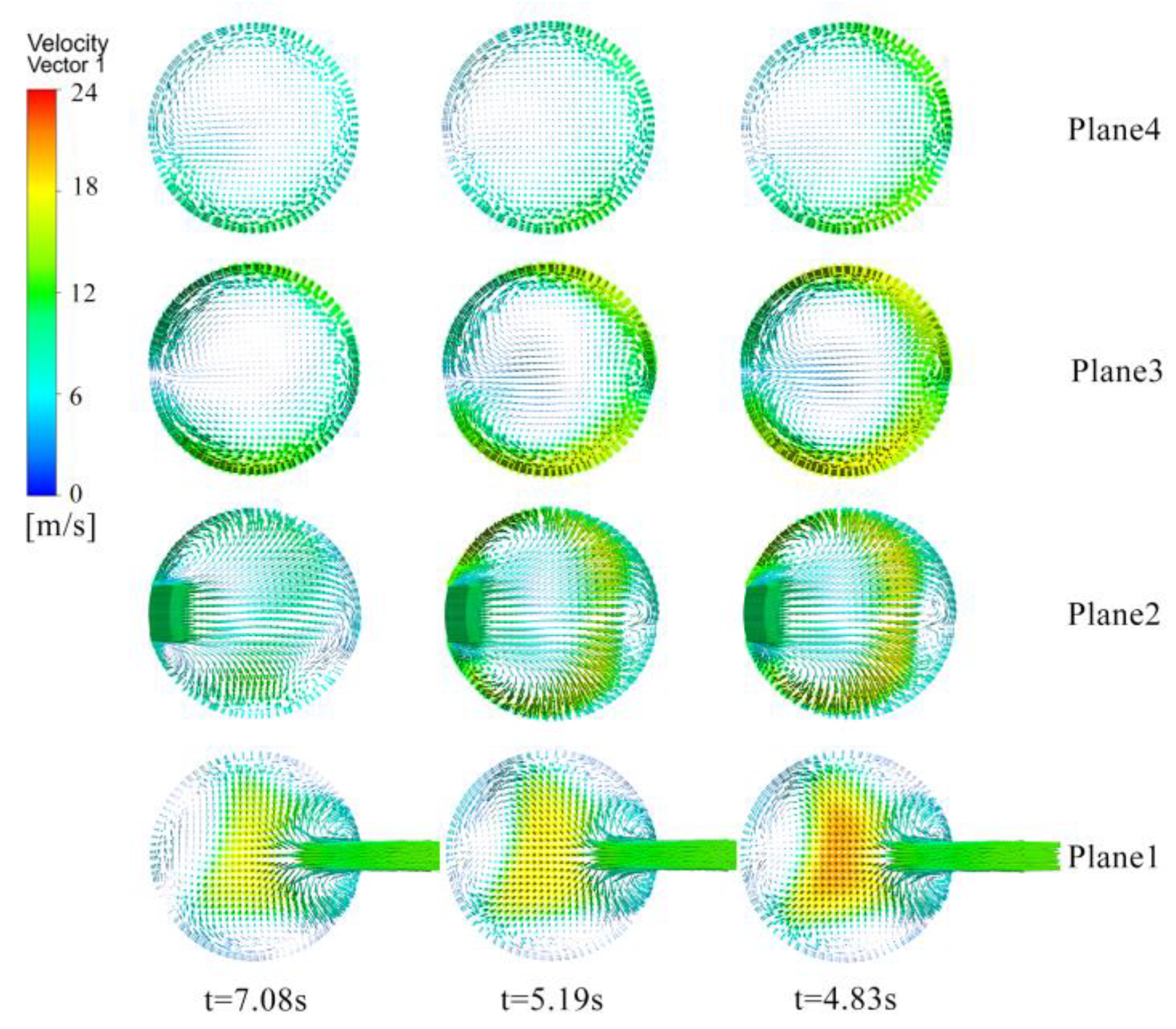
The homogeneous flow model in the reduction furnace is adapted to a more extreme situation. The gas–solid phase mass and heat transfer processes must be fully considered in industrial applications. Hence, the non-homogeneous flow model is more suitable. In the reduction furnace simulation study, the gas–solid phase is modelled as two independent phases. Regarding the existence of the interpenetration phenomenon, previous research has developed a nucleation model, particle model, homogeneous reaction model, structural pore model, and other reaction models applicable to non-homogeneous flow structures. The characteristics of the different gas–solid reaction models are shown in
Table 1.
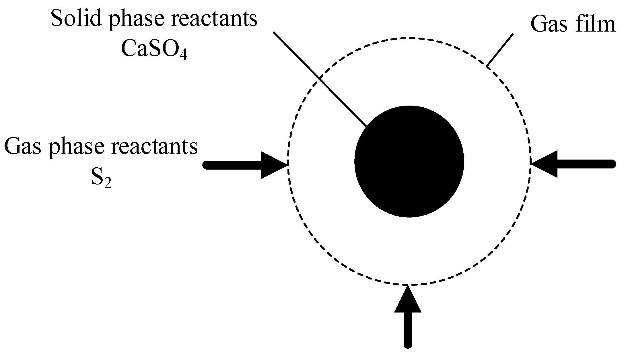
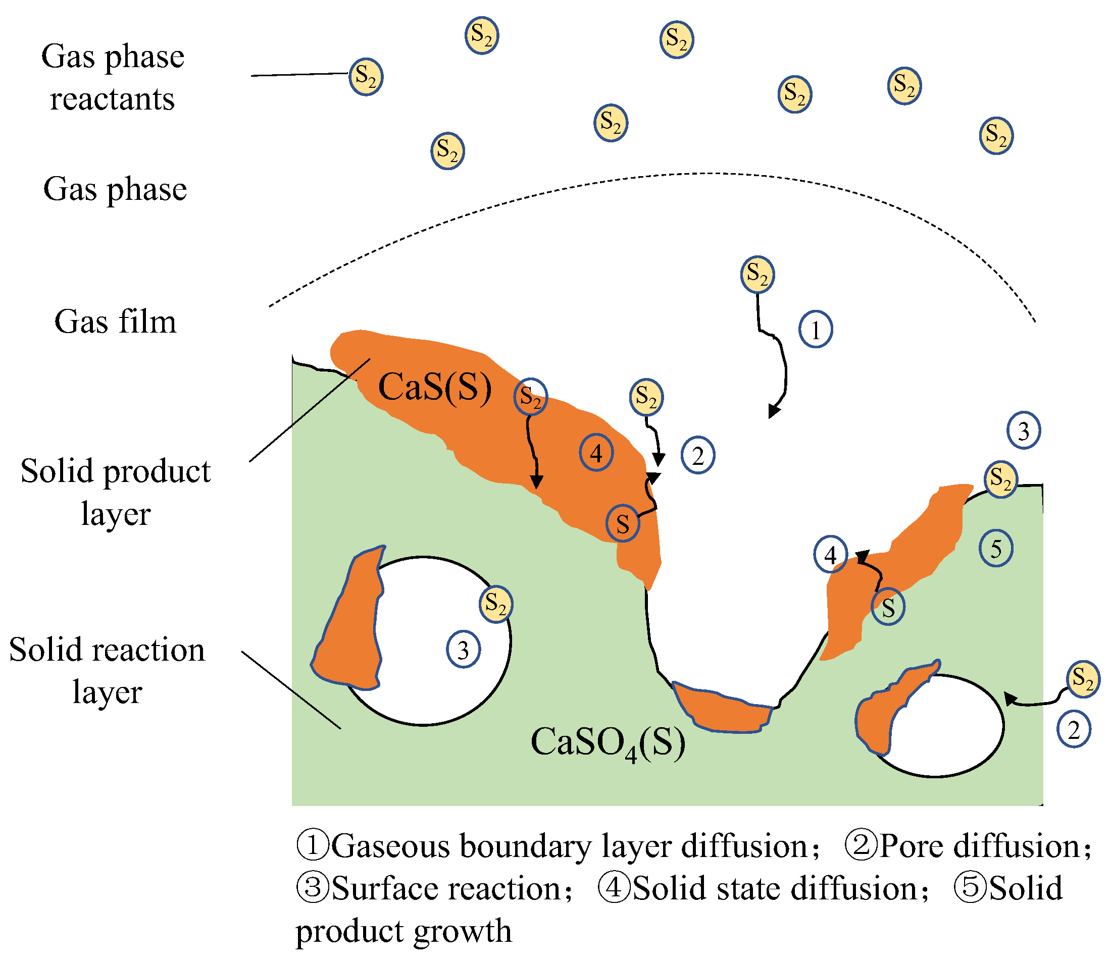
Sohn et al. [
31] first proposed a nucleation model that was used to describe the chemistry of adsorbed gases on porous particles. As shown in
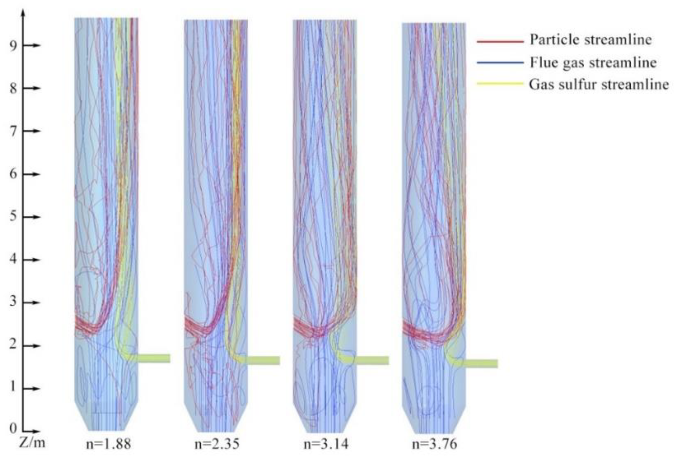
Figure 2 and
Figure 3, the microscopic physicochemical steps in this gas–solid reaction model are similar to those of other models and are usually divided into five steps [
35]. (1) The gas-phase molecules diffuse from the gas-phase main body to the outer surface of solid-phase particles via an external diffusion process. (2) Gas-phase molecules on the surface of solid-phase particles further diffuse through the particle pores (an internal diffusion process). (3) Gas-phase molecules undergo chemical reactions on the surface of local solid-phase particles (a surface reaction process). (4) Reactant molecules diffuse through the product layer and then further react. (5) Solid products gradually grow, leading to solid-phase particle structure changes. These steps proceed simultaneously and are mutually constrained. It is a typical multiscale, multiple physicochemical coupled system.
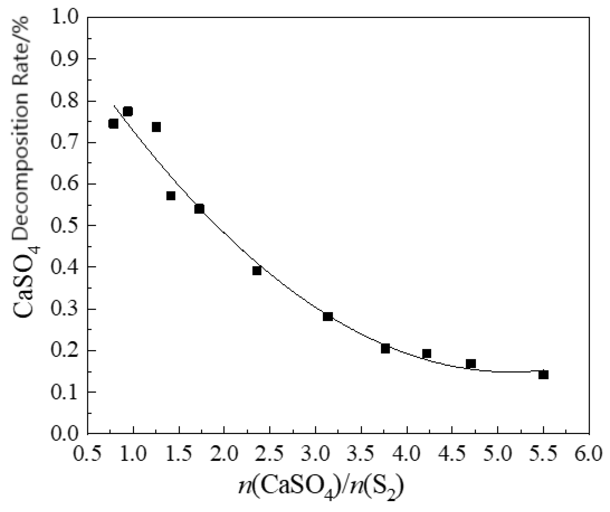
The reaction between gaseous sulfur and CaSO
4 in the reduction furnace is a gas– solid non-catalytic non-homogeneous reaction. Its reaction model is based on the nucleation model of the gas–solid reaction (Equation (8)), wherein the solid-phase reactant nuclei are wrapped with a gas film, while gaseous sulfur reacts with CaSO
4 through the gas film as expressed below:
In this model, the solid-phase particle diameter remains constant during the reduction of CaSO
4 particles by gaseous sulfur, while the particle density decreases. The reaction rate is expressed as:
where
ρs is the density of gaseous sulfur within the CaSO
4 particles (mol/m
3),
R0 is the particle size,
cA,0 and
cA,e are the equilibrium concentrations of gaseous sulfur at the beginning and end of the reaction, respectively (mol/m
3),
f is the conversion rate,
β is the gas film mass transfer coefficient (m/s),
DAB,e is the effective diffusion coefficient (m
2/s),
k is the rate constant of the primary reversible reaction, and
K is the reaction equilibrium constant.
The first, second, and third terms in parentheses are the diffusion resistance of the boundary layer, internal diffusion resistance of the reduced CaSO
4 layer, and resistance of the chemical reaction, respectively. Their relative magnitude varies with the nature of the solid phase particles, ambient fluid velocity, temperature, particle size, and other factors. Furthermore, this leads to the variation in the limiting link during the reduction reaction process. The relative magnitudes of the influence of the aforementioned links can be obtained from the relative magnitudes of
β,
DAB,e, and
k. The common reaction mechanism identification effects are listed in
Table 2 [
36].
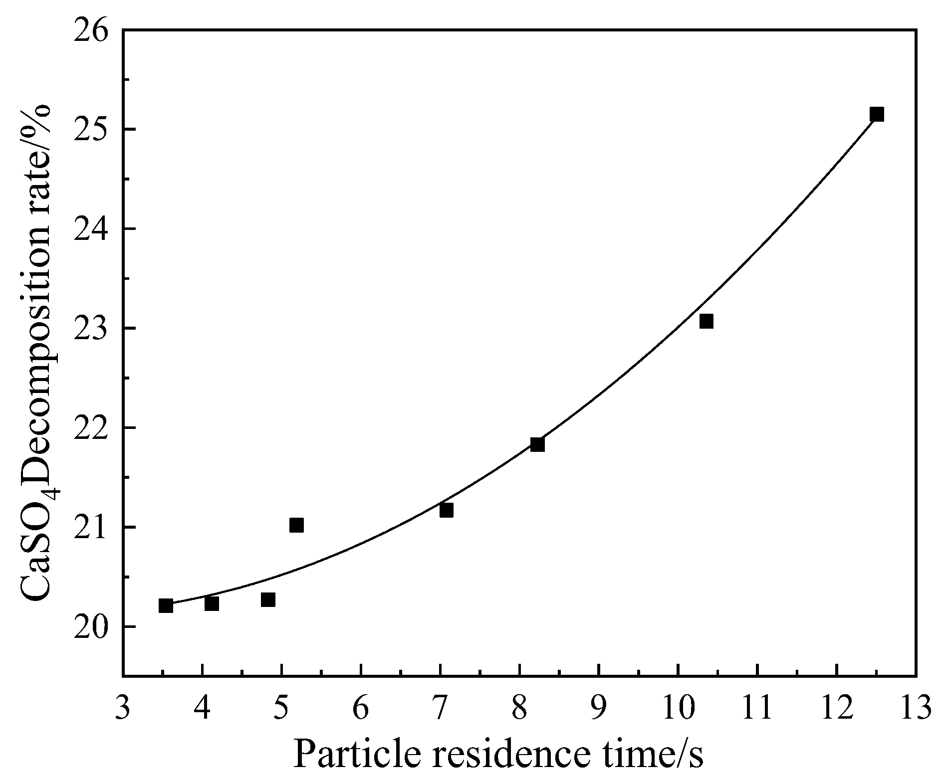
Yan et al. [
37] investigated the kinetics of the high-temperature decomposition of CaSO
4 using a shrinking nucleus model. They concluded that the SO
2 concentration of the reaction system had a significant inhibitory effect on its decomposition. The concentration of SO
2 and O
2 on the surface of the unreacted nucleus increased and decreased as the reaction progressed. The average porosity of the product layer decreased with time, which provides insight into the study of the mechanism of CaSO
4 decomposition. This is why the chemical reaction model studied in this work uses a component transport model based on the nucleation model for the simulation study of CaSO
4 reduction by gaseous sulfur in the reduction furnace.
Similar to the calcium carbonate decomposition model, the CaSO
4 decomposition model is referred to as the calcium carbonate decomposition mechanism. Khinast et al. [
38] showed that both chemical reactions and mass transfer within calcium carbonate particles play a controlling role in the reaction rate. Satterfield and Feakes [
39] conducted thermogravimetric studies on calcium carbonate particles of different sizes and discovered that the thermal decomposition of calcium carbonate in small particles was mainly controlled by chemical reactions. Presently, national and international studies have shown that the decomposition process of fine calcium carbonate powder particles in suspension are mainly controlled by chemical reactions. This conclusion has been affirmed by most scholars. In this study, a gas–solid reaction model based on the nucleation model is established for numerical simulation, and the main reactions in the model are as follows:
Because the reaction mechanism is controlled by a chemical reaction, its boundary and internal diffusion resistance can be neglected. Hence, Equation (9) can be simplified as:
where
ρs,
cA,0, and
cA,e are calculated based on the Fluent component transport model,
R0 is the particle size (obeying the Rosin–Rammler distribution),
K is the equilibrium constant of the reaction,
k is the reaction rate constant obtained from the Arrhenius equation,
f is the conversion rate (
f = (
n0 −
nt)/
n0),
n0 is the initial number of solid reactants moles, and
nt is the number of solid reactants moles at time
t.
The chemical reaction kinetic data for reaction 10 were obtained from the findings in the literature [
13] that the one-step reaction mechanism for the reduction of phosphogypsum by gaseous sulfur is chemically controlled, and the kinetic equation is as follows:
The chemical reaction kinetic data for reaction 11 were derived from the literature [
40], and the chemical reaction kinetic equation is:
The total reaction rate of the gas–solid reaction can be obtained by substituting the data in Equation (14) into (13). The particle size of the solid-phase particles and rate constant of the gas–solid reaction are introduced into the component transport model using Fluent, which accurately describes the gas–solid reaction process which is controlled by the chemical reaction.
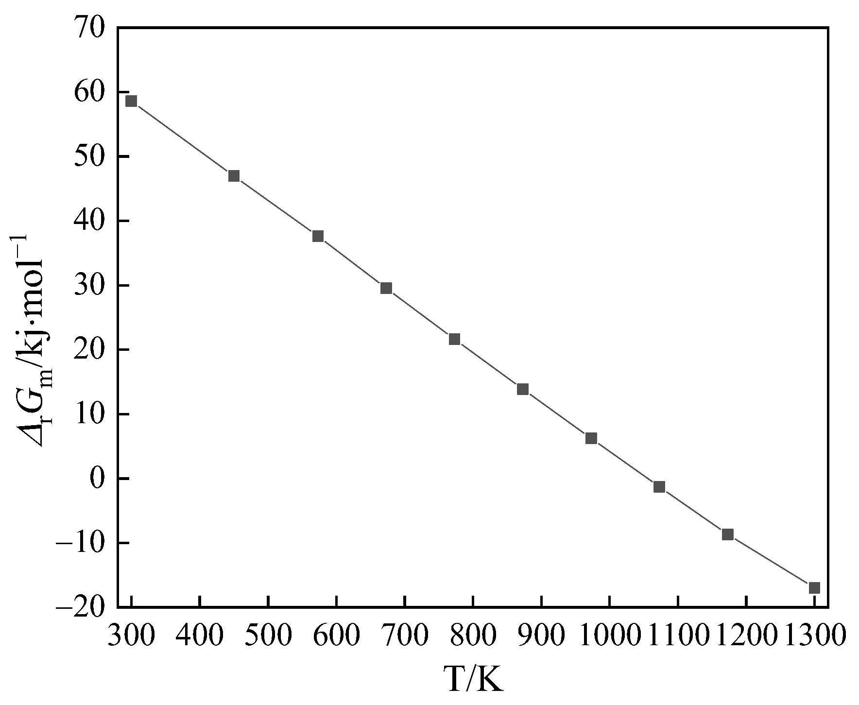
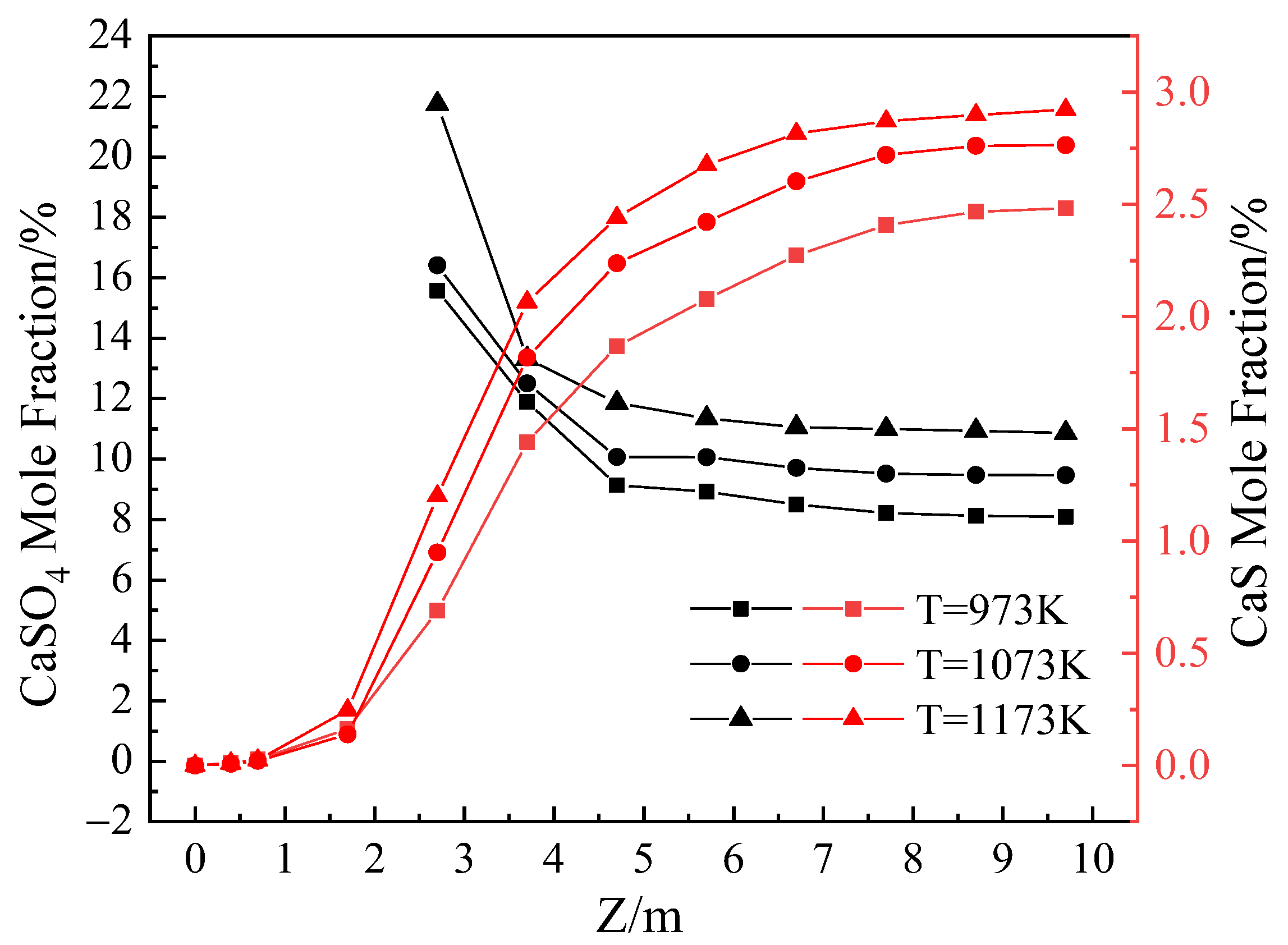
The change in the standard molar reaction Gibbs free energy (Δ
rGm) of reaction 11 is shown in
Figure 4 [
41]. The direction, mode, and priority of the reaction are determined depending on whether Δ
rGm is less than 0. The results of the thermodynamic reaction calculations show that gaseous sulfur and phosphogypsum progressed spontaneously above 1073 K, while the direct thermal decomposition reaction temperature of phosphogypsum was 1573 K. Hence, it did not decompose directly. In this reaction stage, the gaseous sulfur reduction of CaSO
4 to produce CaS is the main reaction. Compared to the occurrence of multiple side reactions in the reduction of phosphogypsum with coke, the temperature control of the sulfur gas in the pre-decomposition stage of CaSO
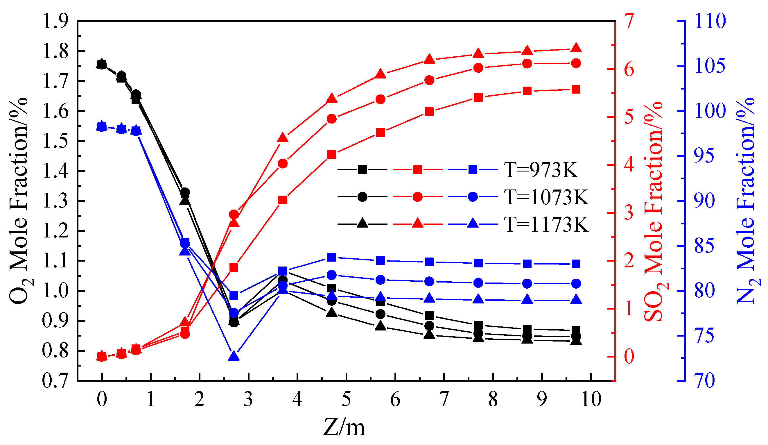
4 is milder, and the reaction temperature is between 1023 and 1223 K.


