Article

Separation of Molar Weight-Distributed Polyethylene Glycols by Reversed-Phase Chromatography—II. Preparative Isolation of Pure Single Homologs

Institute for Separation Science & Engineering, Friedrich-Alexander-Universität Erlangen-Nürnberg, Egerlandstr. 3, 91058 Erlangen, Germany
*
Author to whom correspondence should be addressed.
Processes 2023, 11(3), 946; https://doi.org/10.3390/pr11030946
Submission received: 22 February 2023 / Revised: 16 March 2023 / Accepted: 17 March 2023 / Published: 20 March 2023
(This article belongs to the Section Separation Processes)

Abstract

:
The isolation of single homologs of polyethylene glycol by preparative reversed-phase chromatography is investigated. A thermodynamic model developed accurately previously describes the retention times of individual homologs as function of their size, temperature, and mobile phase composition under linear, diluted conditions. The model is extended to predict limiting retention times for linear gradient operation in preparative applications. Isocratic and gradient-based separations are studied under strongly overloaded conditions. Baseline separation of homologs up to 3000 g/mol is demonstrated. Quantitative production of pure single homologs up to molar weights of 1000 g/mol was performed using an automated setup.

Graphical Abstract

1. Introduction

Producing single homologs of polymers is a challenging, but relevant, problem. Such monodisperse (uniform) polymers have very well-defined properties, which are of high interest in medical, analytical, biotechnological, and chemical applications. However, the synthesis of polymers generally leads to polydispersed products. While modern synthesis protocols can produce polymers with low polydispersity and smaller single homologs, these methods are still tedious [1]. Often, subsequent chromatographic purification is required to narrow down the molar weight distribution (MWD) and removal of impurities [2]. Against this background, the isolation of pure homologs from polydisperse mixtures by chromatography may provide flexible methods for producing single or multiple selected homologs simultaneously on a larger scale.
Polyethylene glycol (PEG), studied here, is a versatile polymer with many applications. Conventional polydisperse PEGs are found in cosmetics, surfactants, and fabric softeners, to name a few. In contrast, PEGs with very narrow MWDs or even single homologs are of high interest in medicine and biopharmaceutical research. Here, they are bound to active drug molecules to control their solubility, stability, and bioavailability [3]. Since polydispersity strongly affects the activity of PEG-ylated drugs, it is critical to use uniform, well-defined PEGs [2,4,5]. Additionally, single homologs are valuable reference materials for analytical purposes, specifically in measurements related to size and mass of molecules [6], for spectroscopic techniques [7], as standards in size exclusion chromatography, etc.
Monodisperse PEGs are commercially available only up to several hundred Da. As already indicated, corresponding synthesis protocols are still laborious; reviews are given in [1,2,8]. Beyond this, PEG standards with relatively low polydispersity are available. However, in all cases, these are expensive standards, and the costs increase rapidly with the MW of the product. In contrast, conventional polydisperse PEGs are cheap bulk products. A chromatographic isolation of single homologs from such mixtures is certainly interesting. As noted already by Bohn and Meier [2], performing this by size exclusion chromatography (SEC) would be a ‘Sisyphean’ task. Indeed, here high-resolution methods are required as provided by interaction-based retention mechanisms [9,10]. The high resolution power of normal phase and reversed-phase chromatography (RP-HPLC) was demonstrated already at the analytical scale [9,11,12,13,14,15]. Further enhancement is possible by minimizing the band broadening of peaks through the use of modern core-shell columns [15]. Another high-resolution method with low peak dispersion is supercritical fluid chromatography (SFC). At the analytical scale, Poulton et al. [16] successfully used SFC to resolve PEGs with 2000 g/mol on a diol column. To our knowledge, SFC is, so far, the only technique that was applied also for the preparative isolations of single PEG homologs. In several studies by Shimada et al. [17,18] and Takahashi et al. [6,19,20], silica-based SFC columns with diameters of up to 10 mm were used to obtain uniform PEGs, with degrees of polymerization up to n = 42 as reference materials.
In a previous work [15], we demonstrated that RP-HPLC using a C18 core-shell column provides a remarkable resolution of PEGs. For example, the baseline resolution of homologs up to at least 5000 g/mol were achieved, corresponding to a degree of polymerization of n = 113. Moreover, a rigorous thermodynamic model and a simple process model were devised that accurately predicted retention times and chromatograms over a wide range of conditions, in terms of MW of the homologs, temperature, and mobile phase composition.
The goal of this work is to extend the approach above to isolate single PEG homologs at a larger scale. To this end, the thermodynamic retention model from [15] is parametrized through pulse experiments using a preparative core-shell column. Along this line, the role of the injection solvent is also investigated. The model is then extended to linear gradient operation. Based on this, single PEG homologs are produced in quantitative isolation runs. Finally, also the separation of larger PEGs is also discussed briefly.

2. Theoretical Background

2.1. Thermodynamic Retention Model

In a previous work [15], a model was established that predicts accurately the separation of PEGs at analytical scale as function of the degree of polymerization, temperature, and acetonitrile content of the eluent. The approach will be applied here to preparative separations. It is summarized below (for details, see [15]).
For the retention factor in linear chromatography, k = t R t 0 / t 0 , with t R as the retention time and t 0 as the void time, holds thermodynamically
ln k = Δ H R T + Δ S * R ,
where Δ H is the standard enthalpy and Δ S * is the apparent entropy (which also includes the contribution of the bed’s void volume); T is temperature, and R is the gas constant. For the measuring retention times of components at different temperatures, Equation (1) allows for determining Δ H and Δ S * from van’t Hoff plots [21]. Furthermore, according to Martin’s rule [22], the retention of a molecule depends on the contributions of it’s building blocks. For a polymer with degree of polymerization, n, this leads to
Δ H = n Δ H r + Δ H e ,
Δ S * = n Δ S r * + Δ S e * .
The subscripts in Equation (2) denote the repeat units (r) and the end groups (e) of the polymer. Martin’s rule was shown to apply very well to PEGs [13,14,15,23,24,25,26]. The parameters Δ H r , Δ H e , Δ S r * , and Δ S e * can be determined from pulse experiments (see Section 4.2).

2.2. Column Model Based on Discrete Convolution

As shown in [15], the retention model above allows for simulating chromatograms for PEGs under linear conditions with high accuracy by discrete convolution. In brief, the chromatogram of a species i, c o u t , i t results from convolving its injection profile, c i n j , i t (here a rectangular pulse), with its pulse response E i t (here a normal distribution defined through the retention time and the stage number, N T P ). The operation is performed efficiently by fast Fourier transform, FFT and can be written as
c o u t , i t = IFFT { FFT c i n j , i t · FFT E i t } ,
where IFFT denotes the inverse transform. More details are given in [15,27,28,29].

2.3. Linear Solvent Strength Theory

The so-called linear solvent strength (LSS) theory [30,31] provides algebraic expressions for the retention times when using linear solvent gradients. In gradient chromatography, the retention factor k i of a component i typically depends exponentially on the modifier concentration (here, the volume fraction of acetonitrile (ACN) in the mobile phase, ϕ ). In the LSS approach, this dependency is simplified by the local approximation
log k i ϕ = log k i , w S i ϕ ,
where k i , w is the extrapolated value of k i for pure water as the mobile phase, and S i is a constant. Based on this, an approximate expression for the retention time can be derived [30,31], which is written here as
t R , i = t 0 + t D + t i n j + 1 S i β ln 1 + S i β t 0 k i , 0 t D ,
where t D is the residence time in the dwell volume and t i n j is the duration of the injection. The slope of the gradient is given by β = ϕ e n d ϕ 0 / t G , with t G as its duration. k i , 0 is the value of k i at the start of the gradient, i.e., at ϕ = ϕ 0 , which holds ln k i , 0 = ln k i , w S i ϕ 0 .

3. Experimental

3.1. Materials

Technical-grade, polydisperse PEG 1000 (average MW 1000 g/mol) was purchased from Merck KGaA. It is wax-like at room temperature, and its purity is not further specified by the supplier. LC/MS measurements (see below) revealed that it consists of 20 quantifiable individual homologs (see Section 4.1).
Acetonitrile (ACN; HPLC grade) was purchased from Fisher Scientific (Schwerte, Germany). Ultrapure water was prepared using a purification unit (Aquinity2, membraPure, Hennigsdorf, Germany). For sample preparation, an analytical scale (BP 221 S, Sartorius, Göttingen, Germany) was used.

3.2. Preparative Chromatography

The preparative-scale experiments were performed using a 100 × 21 mm core-shell column (Kinetex C18, 100 Å, 5 μ m; Phenomenex, Aschaffenburg, Germany), using water/acetonitrile mixtures as eluent under linear and gradient conditions. After each experiment, a forced elution step of 2 min was performed with a concentration of 80 vol% ACN to flush out larger PEGs still residing in the column, followed by an 8 min equilibration at 15 vol% ACN.
A modular setup was used that consisted of a preparative pump (K-1800, Knauer, Berlin, Germany) with a mounted low-pressure binary gradient mixer (Knauer), a 4-port degasser (Knauer), a thermostat (RE 306, Lauda, Lauda-Königshofen Germany), and a fraction collector (Foxy R1, Knauer). Process monitoring was performed by a coupled charged aerosol detector (CAD; Corona Ultra RS, Thermo Fisher Scientific, Waltham, MA, USA) and mass spectrometer (MS; AB SciexQTrap, Sciex, Darmstadt, Germany) for the identification of the individual homologs. The setup was controlled using a custom Python-based software. The column was placed in a thermostated bath. Injection volumes below 1 mL were applied via injection loops installed at a 6-port, 3-channel injection valve (Knauer). For automatization of the injections, the sample solutions were delivered by a feed pump (K-500, Knauer). Injections above 1 mL were realized directly via the pump and gradient mixer. An adjustable semi-preparative post-column flow splitter (ASI, Richmond, CA, USA) split the flow between detectors and fraction collector at a ratio of about 1:20. The smaller flow was again split between CAD and MS using a micro metering valve assembly (IDEX, Northbrook, IL, USA).
For all isocratic experiments, eluent composition was adjusted by weighing corresponding amounts of water and ACN using a precision scale (BP 8100, Sartorius). Degassing was performed by helium sparging. For gradient chromatography, the eluents were mixed by the gradient pump after they passed the online degasser.
When high purity of collected fractions was confirmed, they were pooled according to their degree of polymerization, concentrated in a vacuum rotary evaporator (Laborota 4000/4001 efficient, Heidolph, Schwabach, Germany), and subsequently freeze-dried to powder form by lyophilisation (Alpha 1–4, Martin Christ Gefriertrocknungsanlagen GmbH, Osterode am Harz, Germany).

3.3. Analytical Chromatography

Analysis of samples and collected fractions were performed by LC/MS using an analytical core-shell C18 column (Kinetex C18, 100 × 4.6 mm, 100 Å, 2.6 μ m; Phenomenex) and an Ultimate 3000 LC unit (Dionex, Sunnyvale, CA, USA) consisting of a gradient pump LPG-3400A with internal degasser, column thermostat TCC-3000, and an autosampler WPS-3000SL. The same CAD/MS detection system was used as described above. The analyses were performed under isocratic conditions at 25 °C using water/ACN 80/20 v/v as eluent at a flow rate of 1 mL/min. Injection volume was 10 μ L.

4. Results and Discussion

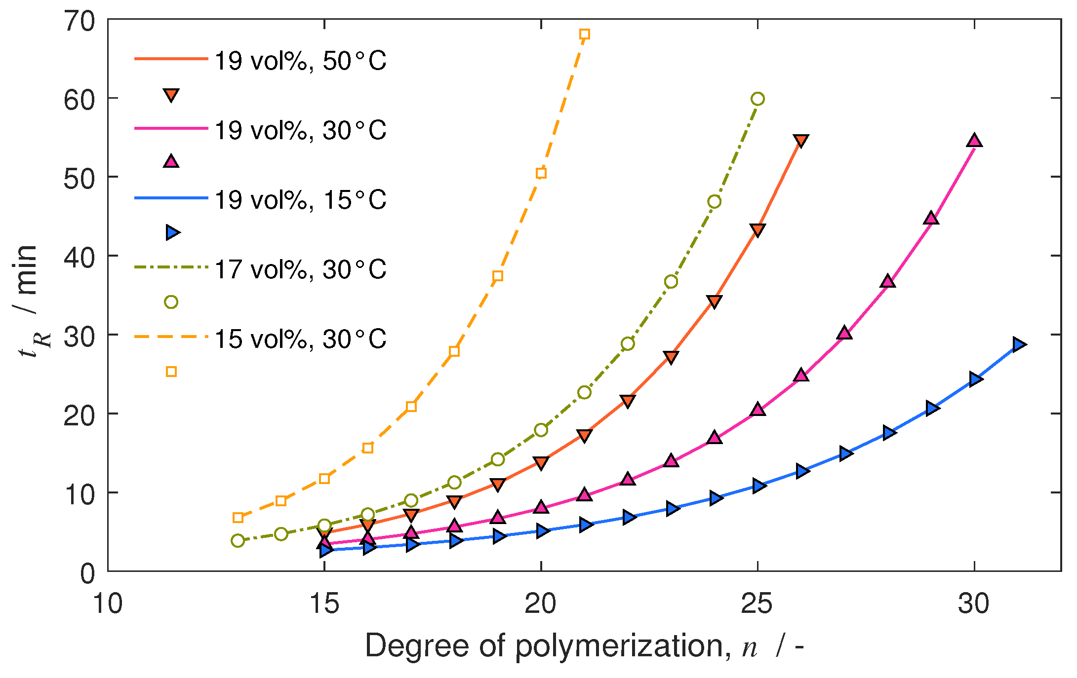
4.1. Separation Problem and Role of Operating Conditions

While our previous study [15] was performed using high-quality narrow PEG standards, the scope here is on the preparative-scale isolation of homologs from inexpensive polydisperse PEGs. Thus, a technical-grade PEG 1000 was chosen as a model system. The analysis of the MWD by LC/MS, shown in Figure 1, reveals that the PEG 1000 contains, in total, 20 quantifiable homologs with degrees of polymerization ranging from n = 13 to n = 32. The polydispersity of the material was calculated as 1.025, which indicates that it has (owing to its low average MW) still a quite narrow MWD. As seen in Figure 1, the MWD is described well by a normal distribution.
To adjust the flow rate for the preparative column, we consider the simplest scale-up method for chromatographic separations. When applying a column with the same packing material and length, but increased diameter, and using the same linear velocity and relative injection volume, very similar chromatograms will result at both scales. For this, the flow rate and injection volume are increased by the scale-up factor D 2 / D 1 2 , where D 1 and D 2 are the diameters of the two columns. The two columns used here have the same length, but due to limit pressure drop for the preparative column, a packing with slightly larger particles (5 μ m, instead of 2.6 μ m) was selected. The scale up factor is 21.2 mm / 0.46 mm 2 = 21.2. Based on this, the flow rate was fixed to 20 mL/min. Depending on ACN level and temperature, pressure at 20 mL/min varied between 65 and 95 bar, which fits the equipment limit of 100 bar.
Figure 2 shows example chromatograms obtained for the preparative column that displays the interaction between the molar weight of the homologs and the chromatographic operating conditions, in terms of temperature and eluent composition. Retention increases strongly with increasing degree of polymerization, n, as well as with increasing temperature and decreasing acetonitrile content. These observations are consistent with the previous results at an analytical scale and discussed in detail in [15].
An important aspect of preparative chromatography is the solvent used for sample injection. It is well-known that injecting a feed mixture in a solvent different from the mobile phase can strongly influence chromatograms. In addition to the potential detrimental effects, such as band splitting or peak deformation, beneficial phenomena, such as peak sharpening, are also possible. To elucidate the role of the injection solvent, a series of experiments was performed using the analytical column with various levels of ACN in the mobile phase. Table 1 summarizes the results for the example of homolog n = 20. For the small injections performed here, the retention factor k is practically constant. This is important, since it allows us to apply the thermodynamic model in Section 2.1 to this kind of operation, as well. However, column efficiency, in terms of the number of theoretical stages, N T P , increases strongly with decreasing ACN level and reaches a remarkable maximum of 14,000 theoretical stages when using pure water for injection. Additionally, peak asymmetry (determined by the conventional method at 5% peak height) is reduced the more water the injection solvent contains. These observations are analogous to those of VanMiddlesworth and Dorsey [32], who studied this for the homologous series of methyl ketones in RP-HPLC.
The reason for this behavior is that sorption increases exponentially here, the weaker the solvent. Thus, the injection in a weak solvent (here water) causes the whole sample to sorb onto the stationary phase in a narrow band at the column inlet. Once the small volume of water has left this zone, the latter is reached by a ’step gradient’ of the stronger ACN-containing eluent, which immediately desorbs all PEGs, causing a highly concentrated, very narrow band that migrates further. Overall, this ’focusing’ phenomenon is analogous to a creating an injection profile much narrower than possible by the experimental setup, leading to very sharp and more symmetrical peaks. A detailed discussion and analysis of the role of the injection solvent in preparative chromatography can be found in the literature [33,34].
As will be shown later, the injection in a weak solvent is also beneficial for the preparative-scale separation of PEGs.

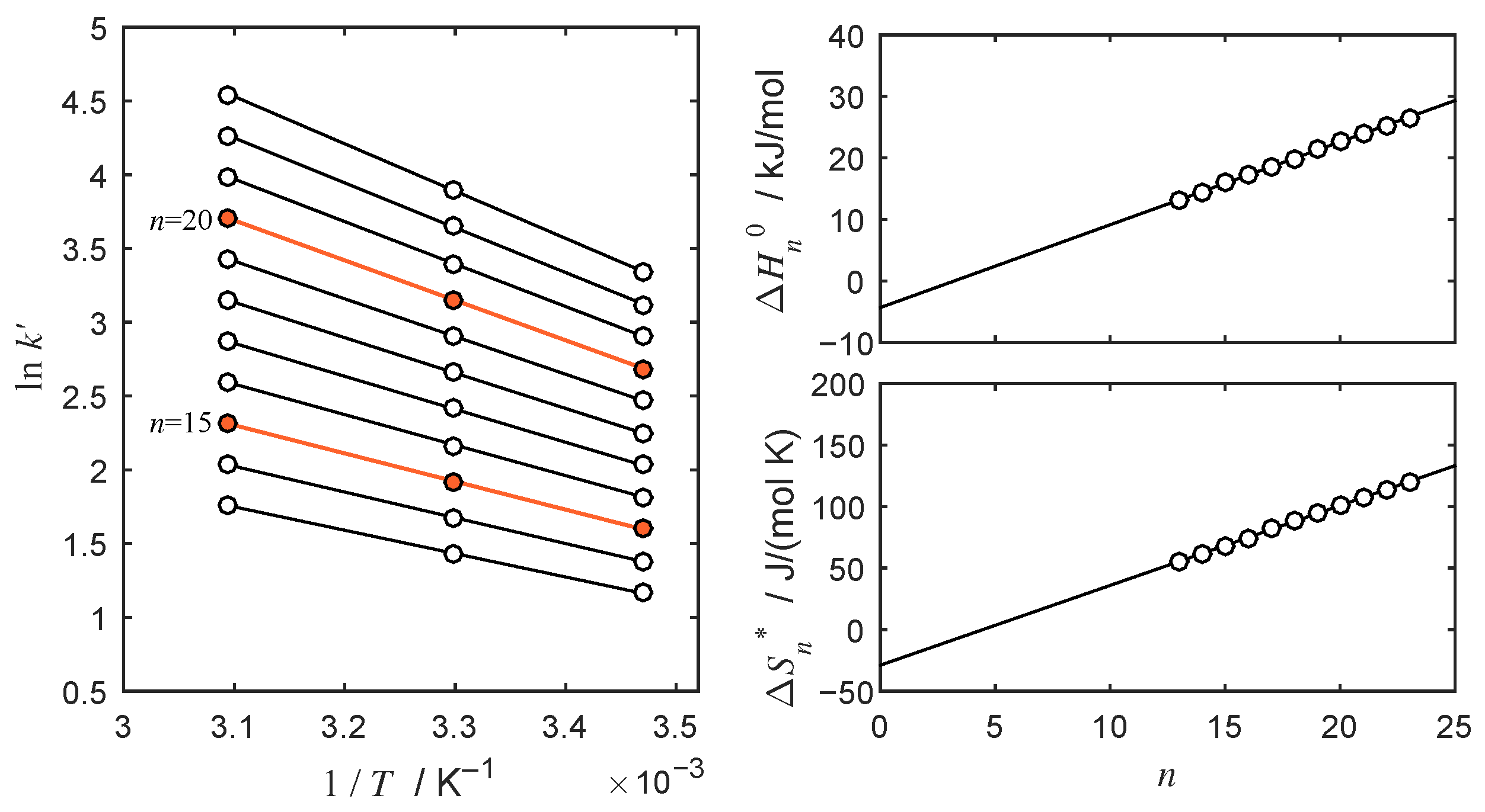
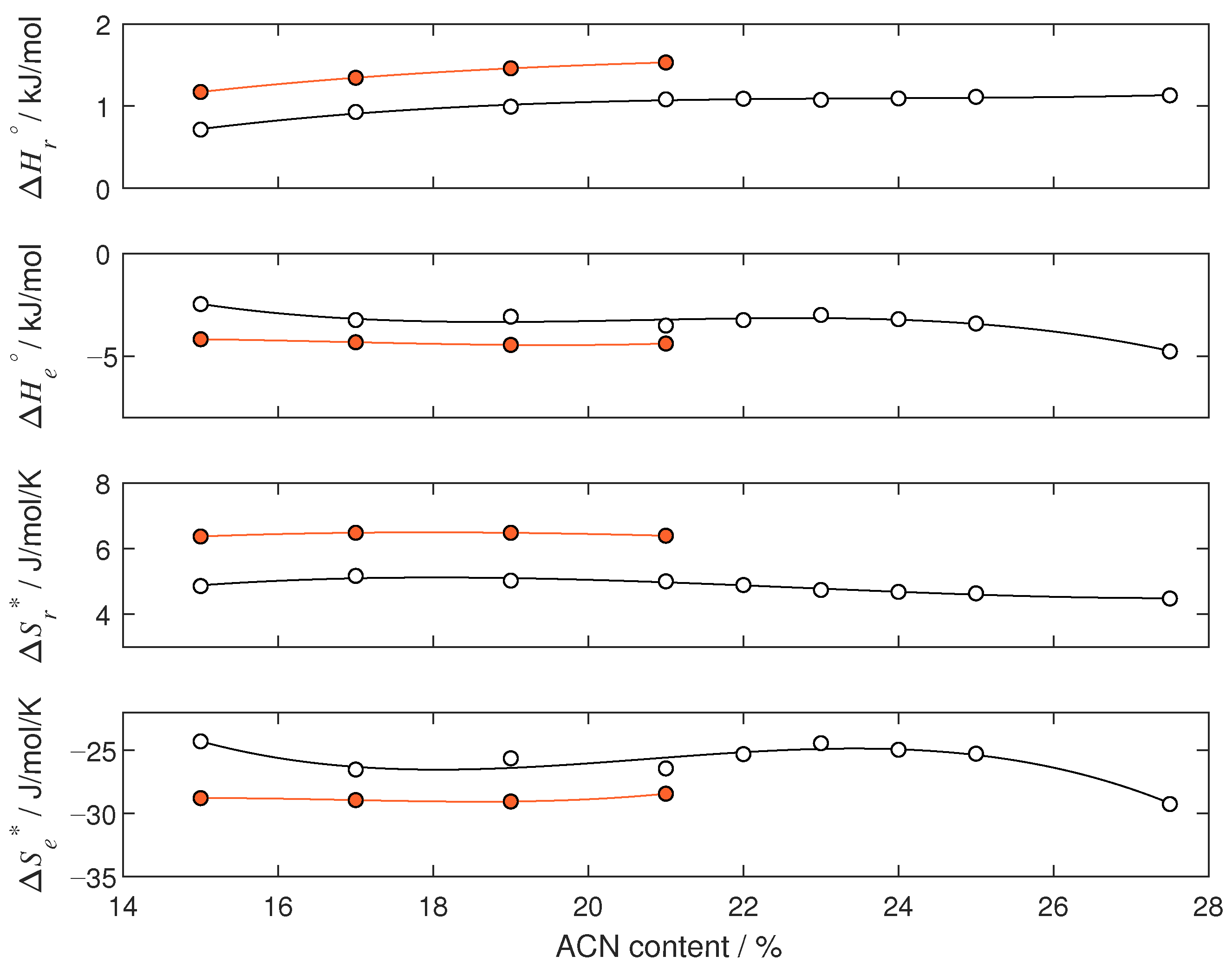
4.2. Thermodynamic Analysis

Following the approach presented in [15], the parameters in Equations (1) and (2) are determined for the preparative column from small pulse injections performed at different temperatures and mobile phase compositions. To ensure linear conditions, small injection amounts (50 μ L of 5 g/L PEG 1000 in water) were applied. In contrast to the analytical-scale analysis in [15] that utilized more than 200 chromatograms, at the preparative scale, the number of experiments must obviously be limited. Here, we evaluate four different acetonitrile contents (15, 17, 19, and 21 vol %) and three different temperatures (15, 30, and 50 C), resulting in a total of 12 chromatograms, which also include the examples shown in Figure 1.
Below, we describe, in brief, the evaluation of the chromatograms; the detailed procedure is given in [15]. First, the retention factors are calculated from the retention times of each homolog n as k i = t R , n t 0 t s y s / t 0 . The required value for t 0 was determined by Trathnigg’s method [24] as t 0 = 0.729 min, and the system’s void time was found by a tracer puls bypassing the column as t s y s = 0.12 min. According to Equation (1), linear regression in van’t Hoff plots, i.e., ln k n vs. 1 / T , then delivers Δ H n and Δ S n * for each homolog. An example is given for an eluent with 17 vol% ACN in Figure 3 (left). The determined Δ H n and Δ S n * are then subjected to linear regression against Equation (2), which gives the enthalpic and entropic contributions for the repetitive units ( Δ H r , Δ S r * ) and end groups ( Δ H e , Δ S e * ). This is exemplified in Figure 3 (right). The procedure works equally well for all ACN concentrations used (corresponding plots for 15, 19, and 21 vol% are given in Figures S1–S3 in the Supplementary Materials). The very good agreement of the linear regressions confirms that the thermodynamic model is applicable to the preparative column.
The obtained thermodynamic parameters are listed as function of the mobile phase composition in Table 2. Figure 4 compares the parameters to those determined in [15] for the analytical column. The parameters for both columns are quite similar and follow the same trends with changing ACN content of the mobile phase. Interestingly, the contributions of the repeating units, Δ H r and Δ S r * , are consistently higher for the preparative column, whereas the values for the end groups, Δ H e and Δ S e * , are lower than for the analytical column. Overall, when calculating values for Δ H and Δ S * for the typical conditions used here, one finds that, in both cases, the entropic contribution is slightly more influential than the enthalpic one. Further, both values are somewhat higher for the preparative column. Nonetheless, the determined k values are similar for both columns, owing to the slightly lower porosity of the larger column. Moreover, as shown in [15], the separation factor between neighboring homologs is given by
ln α = Δ H r R T + Δ S r * R .
when evaluating this expression, one finds strikingly similar separation factors for both columns. For example, at 50 C and 15 vol% ACN (very strong retention), one finds α prep = 1.39 and α analyt = 1.38, while at 15 C and 21 vol% ACN (very weak retention), α prep = 1.13 and α analyt = 1.16 are obtained.
To summarize, the thermodynamic retention model can be applied to the preparative column. The parameters, and in particular, the selectivity for this core-shell column, which has larger particles, are very similar to the analytical column studied earlier.

4.3. Separation under Linear Conditions

Provided the distribution equilibria of the homologs remains in the linear range, which should be the case under sufficiently diluted conditions, the thermodynamic model above predicts retention times very accurately, as demonstrated in Figure 5. Here, the predictions are compared to the experimental retention times for the chromatograms shown in Figure 2. Despite the fact that the measured retention times were part of the data set used for parametrizing the model, the agreement is still striking.
In the next step, we investigate the applicability of the column model based on discrete convolution (see Section 2.2). As explained in [15], the retention model and an expression for the number of theoretical stages, N T P , are sufficient to parametrize the residence distributions E i t needed to apply Equation (3). Figure 6 shows a comparison between the model and two experimental chromatograms measured at conditions that were not used for model parametrization, namely at 20 vol% ACN and 20 C (Figure 6, left) and 20 vol% ACN and 35 C (Figure 6, right). In both cases, the model predicts the experiments with high accuracy, even though equal N T P values were used for all homologs.
In the previous examples, narrow injections of 50 μ L were applied using water as a solvent. As a complementary example, we consider also a large injection volume of 150 mL with the eluent as the injection solvent. Remaining in the linear sorption regime requires the use of a very low injection concentration of 0.05 g/L. Figure 7 shows a resulting chromatogram. It can be seen that the detector signal (black) is very low. Due to the absence of a sharpening effect by the injection solvent (see previous example and discussion in Section 4.1), band broadening is apparently too strong to achieve clear separation. However, the step-wise change of the signal indicates the elution of the broader bands of the homologs. This is also supported by the fact that the retention intervals predicted by the thermodynamic model also fits these steps.
In addition, Figure 7 includes a chromatogram measured under the same conditions, but using an injection solvent with 5 vol% ACN only. Here, the expected sharpening effect occurs and leads to clearly baseline-separated peaks. Notably, their retention times also fall mostly into the predicted elution windows. The shapes of these peaks, however, are strongly asymmetric, indicating a complex interaction of the broad water plug with the sorbed PEG molecules. Furthermore, for the earlier eluting peaks, overlapping elution intervals are predicted (thus, in the figure, only a single early interval is marked), while the peaks, indeed, remain baseline-separated. This indicates the strong benefits of performing injections in weak solvents, but also shows a limitation of the retention model.
While the linear convolution model is obviously not applicable for situations with asymmetric peaks (as is the case for the remainder of this work), it should be noted that the approach is powerful and accurate. In the context of preparative chromatography, it is applicable directly if equilibria can be approximated by linear functions such as, for example, in SEC [28] and in many sugar separations [35].

4.4. Separation under Nonlinear Conditions

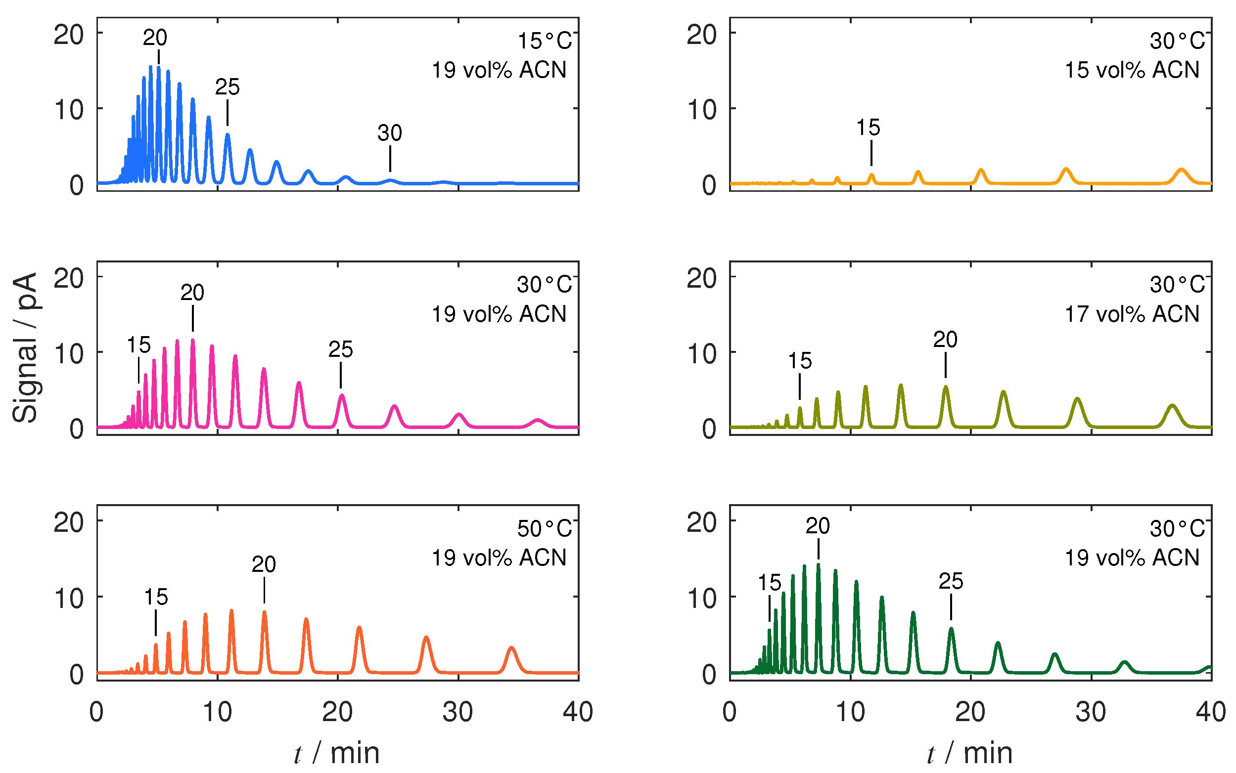
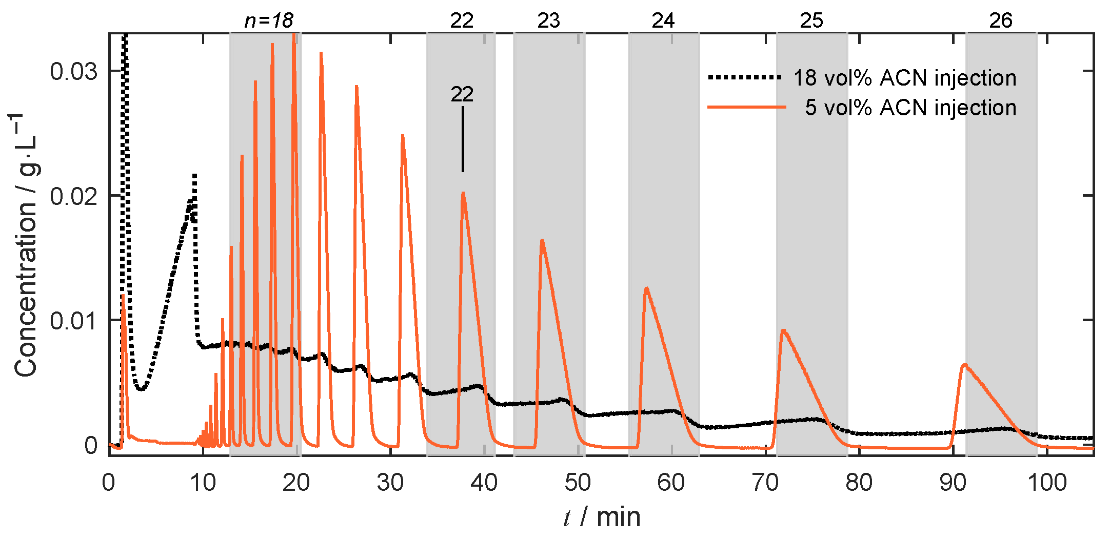
4.4.1. Isocratic Operation

In preparative separations, large injection amounts are used to achieve economic process performance, in terms of throughput and solvent consumption. Below, we investigate the system’s behavior under the corresponding conditions. Figure 8 compares five chromatograms for large injection amounts obtained for a constant injection volume of 500 μ L and increasing injection concentrations between 5 g/L and 100 g/L. It is observed that, in all cases, asymmetric chromatograms result in increasingly sharp fronts and dispersive waves (‘tails’) at their rear. This behavior corresponds to so-called favourable nonlinear sorption isotherms (as is, for example, the well-known Langmuir model). A qualitative comparison of the results to those in Figure 8 also underlines the beneficial role of water as an injection solvent.
The figure also contains the predicted elution times for the selected homologs. It is readily observed that the predicted times fall quite accurately into the end points of the tails (as expected from theory). This underlines that the retention model is also a helpful tool for designing preparative-scale separations under strongly overloaded conditions.
It should be noted that the example in Figure 8 was designed to demonstrate the fundamental behavior at short run times to save eluent. For this, intermediate values for temperature and ACN level were chosen. As shown in [15], this significantly limits the selectivity and achievable resolution. Nonetheless, even under these conditions, large injection amounts can be separated. Baseline resolution is achieved (for some peaks), even when injecting 25 mg PEG 1000 (50 g/L). For comparison, injected amounts for Figure 2 and Figure 6 were 0.25 mg, with 7.5 mg in the case of Figure 7. As an example, when assuming an injection concentration of 40 g/L and a run time of 25 min (including a regeneration step), the specific productivity for homolog n = 22 would be about 3.5 g/d/L (grams per day and liters column volume). This may be seen as a low value, but it appears acceptable for valuable reference standards, of which several can be produced simultaneously, since multiple homologs can be isolated from the same run. Furthermore, the separation of significantly larger amounts (and larger homologs, as shown later) is possible by using lower ACN levels and higher temperatures. However, this is at the cost of much longer run times, which, in turn, increases eluent consumption. Correspondingly, finding suitable operating parameters is a non-trivial optimization problem, even for isocratic separations. This is beyond the scope of this work and the subject of ongoing investigations.
It deserves to be mentioned that, due to the strong sensitivity of sorption, with respect to the ACN content of the mobile phase, even slight inaccuracies of the gradient pump (which are typical for preparative-scale equipment) led to significant deviations. Acceptable reproducibility was obtained only by careful premixing of the solvent using a balance.
Apart from this, the separation demonstrated above is seen as a promising example that motivates a further development of corresponding separations.

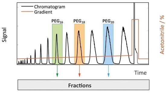
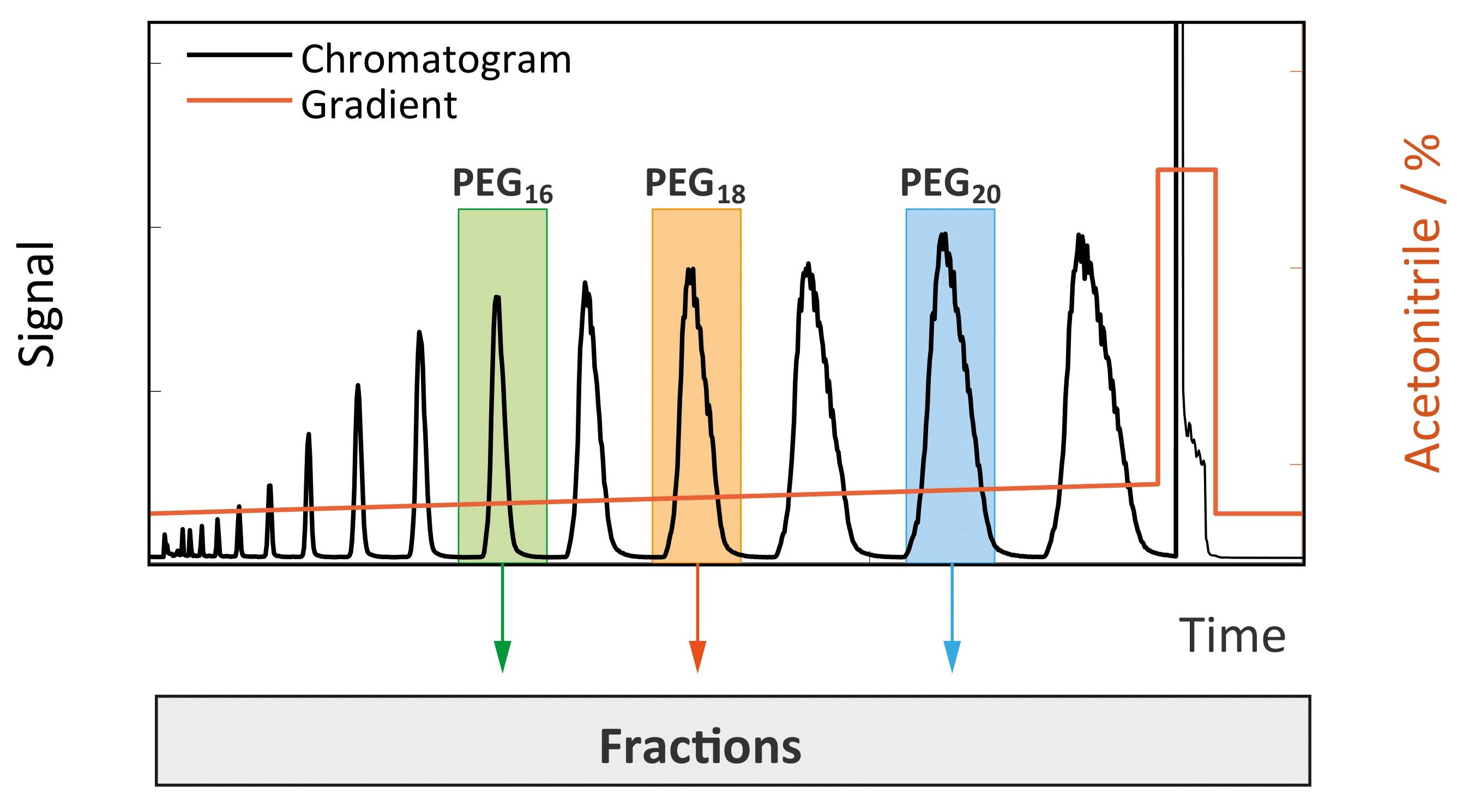
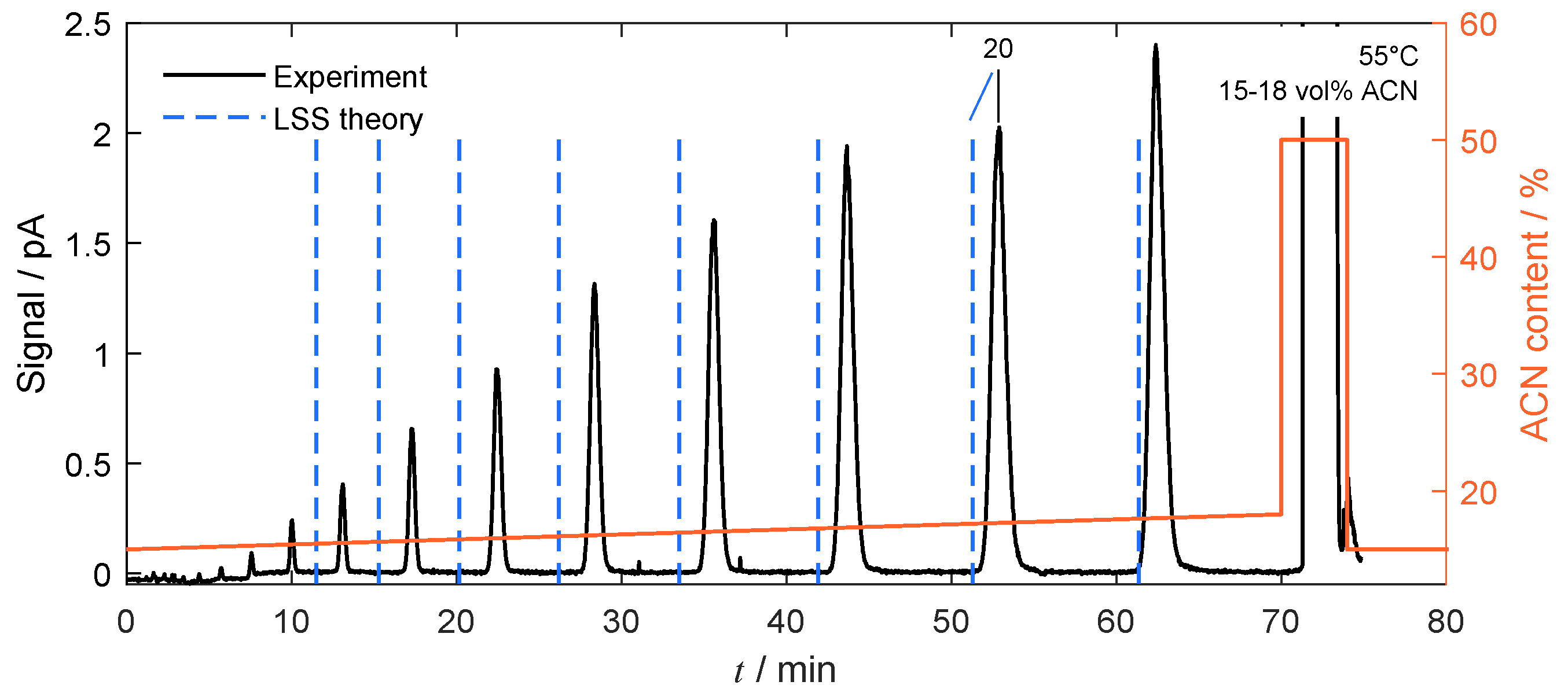
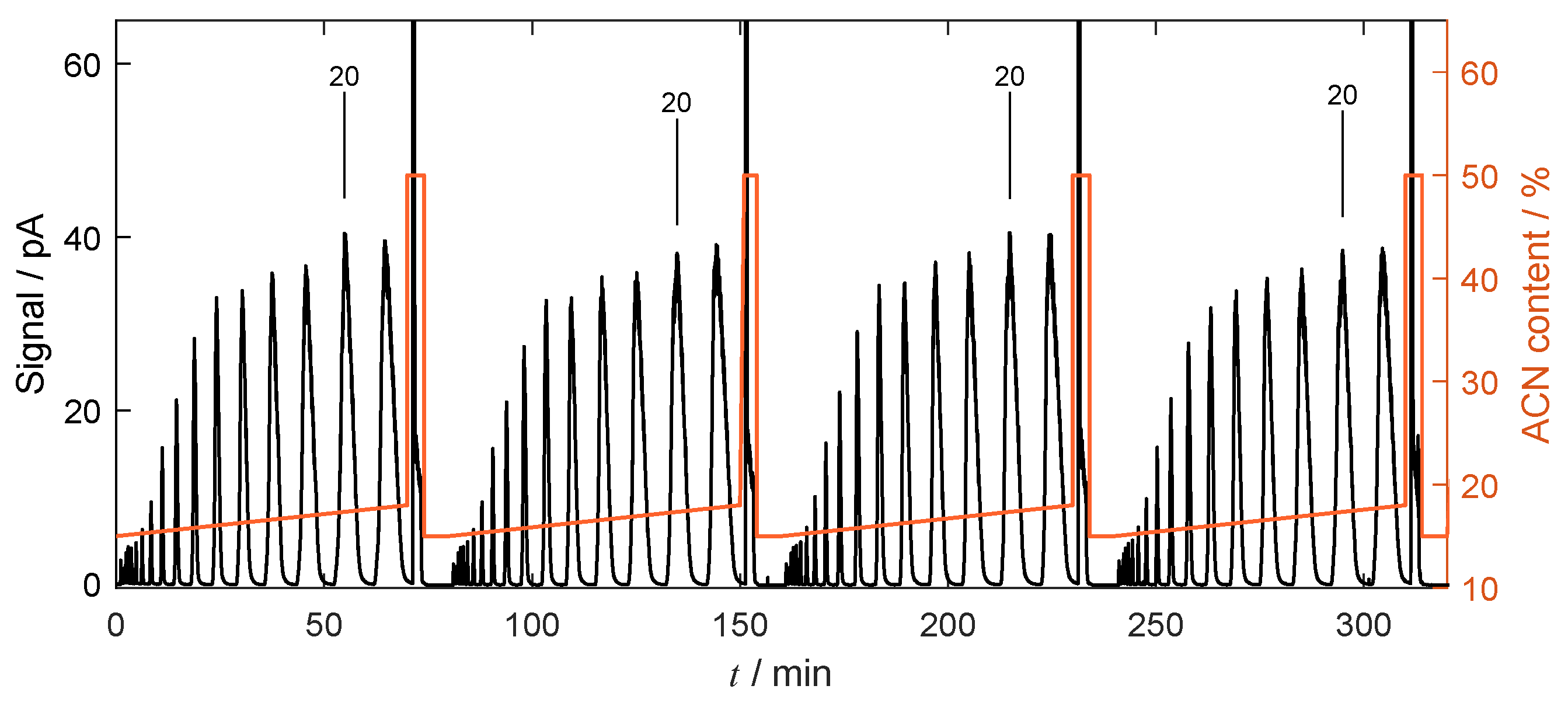
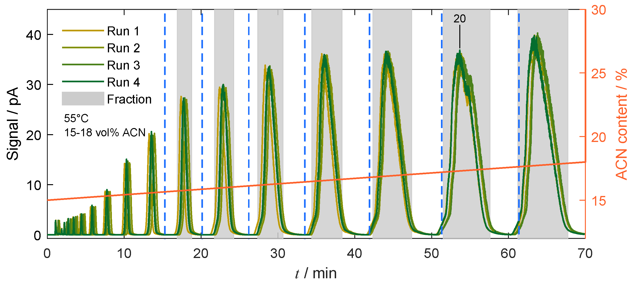
4.4.2. Gradient-Based Operation

The sensitivity of the operation discussed above can be attenuated by applying solvent gradients [30]. Below, experiments with linear ACN gradients are performed to prove the feasibility of a quantitative isolation of individual homologs in high purity. Specifically, the goal is to simultaneously isolate the early-eluting homologs with n = 15 to n = 21, which are present in relatively large amounts in PEG 1000 (see Figure 1). Moreover, the purity of the collected homologs should be maximized, since they are intended as reference materials. Thus, we aim at rather evenly distributed, baseline-separated peaks with additional safety margins between them, which also simplifies automatic peak detection by the fraction collector. A helpful design tool for this is the combination of the retention model (Section 4.2) with LSS theory (Section 2.3) to predict the retention times in the limit of low concentrations.
Figure 9 shows a linear gradient experiment performed under diluted conditions that was designed correspondingly. The chosen, rather flat, gradient leads to good resolution between neighboring homologs. The retention times are distributed rather evenly, with slightly increasing differences to account for the increasing bandwidth of the later eluting homologs. The predictions by LSS theory are shown in Figure 9. To apply this method, the two parameters in Equation (4), k i , w , and S i were fitted for each homolog i by linear regression to the corresponding values from the thermodynamic model. The obtained sets of k i , w and S i fit the thermodynamic model very well (a comparison is given in Figure S4 in the Supplementary Materials). The agreement in Figure 9 between experimental retention times and those calculated from Equation (5) is considered good, in particular, when considering the sensitivity of the system and the existing experimental uncertainties.
Based on this result, linear gradient runs were designed for preparative purposes using the same gradient as in Figure 9, but with increased injection concentrations. Figure 10 shows a series of four consecutive runs, performed using the automated setup with a large injection concentration of 250 g/L (corresponding to 12.5 mg PEG 1000 per injection). As intended, the target peaks are baseline separated, and their increasing bandwidth is accounted for, such that resolution between neighbouring peaks is very similar. There is no sign for deterioration of performance from cycle-to-cycle, leading to good reproducibility.
Finally, the same conditions were applied in collection runs with automated fractionation of the target homologs. Figure 11 shows an overlay of four corresponding runs, with the individual fractions highlighted. The reproducibility is considered very good. The figure also contains the retention times calculated from LSS (blue dashed lines). They, again, agree well with the experiments, but the experimental peaks elute somewhat later than predicted. This indicates that the LSS approach provides useful estimates for the initial design, but is not applicable for a detailed design of such experiments.
The individual eluting homologs were identified by online MS, such that the collected fractions could be allocated and pooled. Figure 12 shows the analyses of the injected mixture and the pooled fractions performed using the analytical column. All fractions are found to contain only the target homolog. The pure homologs were freeze-dried to obtain them in powder form. Subsequently, they were applied as reference standards for, among others, chromatographic experiments and for the development of diffusion measurement by heterodyne dynamic light scattering [7].
Finally, to assess the limits of the approach, gradient-based separations of larger PEGs were also performed. As an example, Figure 13 shows the separation of PEG 4000 into single homologs up to a degree of polymerization of n = 70, corresponding to a molar weight of 3100 g/mol. The more complex gradient used here was designed based on practical experience. Specifically, the later eluting homologs are baseline separated. It is noted that, despite the fact that the injected amount was similar to the examples above, the outlet concentrations are very low, due to band broadening and large retention times. Moreover, the sample contains hundreds of homologs, which translates into small proportions of the individual homologs.
Although the operating conditions in the examples above were not optimized against performance criteria, the results underline the remarkable separation power of RP-HPLC, in conjunction with the efficiency of modern columns also under conditions typical for preparative chromatography.

5. Summary and Conclusions

The applicability of reversed-phase chromatography for the preparative isolation of individual PEG homologs was investigated experimentally.
In a first step, pulse experiments were performed to assess the separation. Along this line, it was found that using a weak solvent for injection causes a ‘focusing’ effect that does not affect retention, but improves separation significantly by peak sharpening. From the pulse experiments, a thermodynamic retention model, devised in [15], was parametrized. Under diluted conditions, retention times and chromatograms were predicted with high accuracy as functions of the size of the homologs, temperature, and mobile phase compositions. The approach is directly applicable to other polymers, provided their retention follows Martin’s rule.
Next, the separation capacity of the column was evaluated using large injection amounts in isocratic operation. Baseline separation of the homologs could be achieved for large injection amounts, even under conditions that favor low cycle times, rather than resolution. The retention model agreed well with the observed dispersive waves of the peaks, making it useful for basic design. However, process stability was limited, due to the exponential dependency of the retention on the acetonitrile content in the mobile phase.
Robustness was enhanced by using linear solvent gradients, for which limiting retention times could be predicted using the retention model and LSS theory. This facilitated designing preparative experiments with shallow gradients and an automated fraction collection that delivered multiple pure PEG homologs simultaneously with molar weights up to 1000 g/mol (n = 21). Finally, the applicability to larger PEGs was confirmed by a gradient-based separation of PEG 4000, where the baseline resolution was achieved for homologs up to n = 70.
The obtained results underline that preparative chromatography may be a useful tool for the isolation of single homologs from polydisperse polymers. The optimization of operating conditions and the use of advanced operating concepts may enhance performance sufficiently to allow for economic productions of single homologs up to a certain size.

Supplementary Materials

The following supporting information can be downloaded at: https://www.mdpi.com/article/10.3390/pr11030946/s1.

Author Contributions

Conceptualization, M.S. and M.K.; data curation, M.S., R.J., B.B. and M.K.; formal analysis, M.S., R.J., B.B. and M.K.; investigation, M.S., R.J. and B.B.; methodology, M.S., R.J., B.B. and M.K.; resources, M.K.; validation, M.S.; writing—original draft, M.S. and M.K.; Writing—review and editing, M.S., R.J., B.B. and M.K. All authors have read and agreed to the published version of the manuscript.

Funding

This work was funded by the Deutsche Forschungsgemeinschaft (DFG, German Research Foundation)—project ID 416229255—SFB 1411.

Institutional Review Board Statement

Not applicable.

Informed Consent Statement

Not applicable.

Data Availability Statement

Not applicable.

Acknowledgments

The authors are grateful to Anna Brünner and Jan-Christoph Domagala for their help with some of the experiments.

Conflicts of Interest

The authors declare no conflict of interest.

References

  1. Trinh, T.T.; Laure, C.; Lutz, J.F. Synthesis of Monodisperse Sequence-Defined Polymers Using Protecting-Group-Free Iterative Strategies. Macromol. Chem. Phys. 2015, 216, 1498–1506. [Google Scholar] [CrossRef] [Green Version]
  2. Bohn, P.; Meier, M.A.R. Uniform poly(ethylene glycol): A comparative study. Polym. J. 2020, 52, 165–178. [Google Scholar] [CrossRef]
  3. Knop, K.; Hoogenboom, R.; Fischer, D.; Schubert, U. Poly(ethylene glycol) in Drug Delivery: Pros and Cons as Well as Potential Alternatives. Angew. Chem. Int. Ed. 2010, 49, 6288–6308. [Google Scholar] [CrossRef]
  4. Yu, Z.; Bo, S.; Wang, H.; Li, Y.; Yang, Z.; Huang, Y.; Jiang, Z.X. Application of Monodisperse PEGs in Pharmaceutics: Monodisperse Polidocanols. Mol. Pharm. 2017, 14, 3473–3479. [Google Scholar] [CrossRef]
  5. Wu, T.; Chen, K.; He, S.; Liu, X.; Zheng, X.; Jiang, Z.X. Drug Development through Modification of Small Molecular Drugs with Monodisperse Poly(ethylene glycol)s. Org. Process. Res. Dev. 2020, 24, 1364–1372. [Google Scholar] [CrossRef]
  6. Takahashi, K. Advanced reference materials for the characterization of molecular size and weight. J. Phys. Mater. 2020, 1193, 146–150. [Google Scholar] [CrossRef]
  7. Wu, W.; Supper, M.; Rausch, M.H.; Kaspereit, M.; Fröba, A.P. Mutual Diffusivities of Binary Mixtures of Water and Poly(ethylene) Glycol from Heterodyne Dynamic Light Scattering. Int. J. Thermophys. 2022, 43, 177. [Google Scholar] [CrossRef]
  8. Zhang, H.; Li, X.; Shi, Q.; Li, Y.; Xia, G.; Chen, L.; Yang, Z.; Jiang, Z.X. Highly Efficient Synthesis of Monodisperse Poly(ethylene glycols) and Derivatives through Macrocyclization of Oligo(ethylene glycols). Angew. Chem. Int. Ed. 2015, 54, 3763–3767. [Google Scholar] [CrossRef] [PubMed]
  9. Sun, C.; Baird, M.; Simpson, J. Determination of poly(ethylene glycol)s by both normal-phase and reversed-phase modes of high-performance liquid chromatography. J. Chromatogr. A 1998, 800, 231–238. [Google Scholar] [CrossRef]
  10. Chang, T. Polymer characterization by interaction chromatography. J. Polym. Sci. B Polym. Phys. 2005, 43, 1591–1607. [Google Scholar] [CrossRef]
  11. Meyer, T.; Harms, D.; Gmehling, J. Analysis of polyethylene glycols with respect to their oligomer distribution by high-performance liquid chromatography. J. Chromatogr. A 1993, 645, 135–139. [Google Scholar] [CrossRef]
  12. Rissler, K. Improved separation of polyethylene glycols widely differing in molecular weight range by reversed-phase high performance liquid chromatography and evaporative light scattering detection. Chromatographia 1999, 49, 615–620. [Google Scholar] [CrossRef]
  13. Cho, D.; Park, S.; Hong, J.; Chang, T. Retention mechanism of poly(ethylene oxide) in reversed-phase and normal-phase liquid chromatography. J. Chromatogr. A 2003, 986, 191–198. [Google Scholar] [CrossRef]
  14. Trathnigg, B.; Veronik, M. A thermodynamic study of retention of poly(ethylene glycol)s in liquid adsorption chromatography on reversed phases. J. Chromatogr. A 2005, 1091, 110–117. [Google Scholar] [CrossRef] [PubMed]
  15. Supper, M.; Heller, K.; Söllner, J.; Sainio, T.; Kaspereit, M. Separation of Molar Weight-Distributed Polyethylene Glycols by Reversed-Phase Chromatography—Analysis and Modeling Based on Isocratic Analytical-Scale Investigations. Processes 2022, 10, 2160. [Google Scholar] [CrossRef]
  16. Poulton, A.M.; Poulten, R.C.; Baldaccini, A.; Gabet, A.; Mott, R.; Treacher, K.E.; Roddy, E.; Ferguson, P. Towards improved characterisation of complex polyethylene glycol excipients using supercritical fluid chromatography-evaporative light scattering detection-mass spectrometry and comparison with size exclusion chromatography-triple detection array. J. Chromatogr. A 2021, 1638, 461839. [Google Scholar] [CrossRef] [PubMed]
  17. Shimada, K.; Nagahata, R.; Kawabata, S.I.; Matsuyama, S.; Saito, T.; Kinugasa, S. Evaluation of the quantitativeness of matrix-assisted laser desorption/ionization time-of-flight mass spectrometry using an equimolar mixture of uniform poly(ethylene glycol) oligomers. J. Mass Spectrom. 2003, 38, 948–954. [Google Scholar] [CrossRef] [PubMed]
  18. Shimada, K.; Kato, H.; Saito, T.; Matsuyama, S.; Kinugasa, S. Precise measurement of the self-diffusion coefficient for poly(ethylene glycol) in aqueous solution using uniform oligomers. J. Chem. Phys. 2005, 122, 244914. [Google Scholar] [CrossRef] [PubMed]
  19. Takahashi, K.; Matsuyama, S.; Saito, T.; Kato, H.; Kinugasa, S.; Yarita, T.; Maeda, T.; Kitazawa, H.; Bounoshita, M. Calibration of an evaporative light-scattering detector as a mass detector for supercritical fluid chromatography by using uniform Poly(ethylene glycol) oligomers. J. Chromatogr. A 2008, 1193, 146–150. [Google Scholar] [CrossRef]
  20. Takahashi, K.; Kishine, K.; Matsuyama, S.; Saito, T.; Kato, H.; Kinugasa, S. Certification and uncertainty evaluation of the certified reference materials of poly(ethylene glycol) for molecular mass fractions by using supercritical fluid chromatography. Anal. Bioanal. Chem. 2008, 391, 2079–2087. [Google Scholar] [CrossRef]
  21. Chester, T.L.; Coym, J.W. Effect of phase ratio on van’t Hoff analysis in reversed-phase liquid chromatography, and phase-ratio-independent estimation of transfer enthalpy. J. Chromatogr. A 2003, 1003, 101–111. [Google Scholar] [CrossRef] [PubMed]
  22. Martin, A.J.P. Some Theoretical Aspects of Partition Chromatography. Symposia Biochem. Soc. 1949, 3, 4–20. [Google Scholar]
  23. Lochmüller, C.; Moebus, M.A.; Liu, Q.; Jiang, C.; Elomaa, M. Temperature Effect on Retention and Separation of Poly(ethylene glycol)s in Reversed-Phase Liquid Chromatography. J. Chromatogr. Sci. 1996, 34, 69–76. [Google Scholar] [CrossRef] [Green Version]
  24. Trathnigg, B.; Skvortsov, A. Determination of the accessible volume and the interaction parameter in the adsorption mode of liquid chromatography. J. Chromatogr. A 2006, 1127, 117–125. [Google Scholar] [CrossRef]
  25. Trathnigg, B.; Jamelnik, O. Characterization of different reversed phase systems in liquid adsorption chromatography of polymer homologous series. J. Chromatogr. A 2007, 1146, 78–84. [Google Scholar] [CrossRef] [PubMed]
  26. Nguyen Viet, C.; Trathnigg, B. Determination of thermodynamic parameters in reversed phase chromatography for polyethylene glycols and their methyl ethers in different mobile phases. J. Sep. Sci. 2010, 33, 464–474. [Google Scholar] [CrossRef]
  27. Villermaux, J. Chemical engineering approach to dynamic modelling of linear chromatography: A flexible method for representing complex phenomena from simple concepts. J. Chromatogr. A 1987, 406, 11–26. [Google Scholar] [CrossRef]
  28. Nguyen, H.S.; Kaspereit, M.; Sainio, T. Intermittent recycle-integrated reactor-separator for production of well-defined non-digestible oligosaccharides from oat β-glucan. Chem. Eng. J. 2021, 410, 128352. [Google Scholar] [CrossRef]
  29. Nicoud, R.M. Chromatographic Processes: Modeling, Simulation, and Design; Cambridge Series in Chemical Engineering; Cambridge University Press: Cambridge, UK, 2015. [Google Scholar] [CrossRef] [Green Version]
  30. Guiochon, G.; Shirazi, D.G.; Felinger, A.; Katti, A.M. Fundamentals of Preparative and Nonlinear Chromatography, 2nd ed.; Academic Press: Boston, MA, USA, 2006. [Google Scholar]
  31. Snyder, L.R.; Dolan, J.W. High-Performance Gradient Elution: The Practical Application of the Linear-Solvent-Strength Model; John Wiley & Sons: Hoboken, NJ, USA, 2007. [Google Scholar]
  32. Van Middlesworth, B.J.; Dorsey, J.G. Quantifying injection solvent effects in reversed-phase liquid chromatography. J. Chromatogr. A 2012, 1236, 77–89. [Google Scholar] [CrossRef]
  33. Ströhlein, G.; Morbidelli, M.; Rhee, H.K.; Mazzotti, M. Modeling of modifier-solute peak interactions in chromatography. AIChE J. 2006, 52, 565–573. [Google Scholar] [CrossRef]
  34. Gedicke, K.; Antos, D.; Seidel-Morgenstern, A. Effect on separation of injecting samples in a solvent different from the mobile phase. J. Chromatogr. A 2007, 1162, 62–73. [Google Scholar] [CrossRef] [PubMed]
  35. Lei, H.; Bao, Z.; Xing, H.; Yang, Y.; Ren, Q.; Zhao, M.; Huang, H. Adsorption Behavior of Glucose, Xylose, and Arabinose on Five Different Cation Exchange Resins. J. Chem. Eng. Data 2010, 55, 735–738. [Google Scholar] [CrossRef]
Figure 1. MWD of PEG 1000 determined by LC/MS (symbols) and interpolation by a normal distribution (line; mean value 22.285, standard deviation 3.81). Measured using the analytical column (eluent 20 vol% ACN, 1 mL/min; 25 C; injection 10 μ L of 1 g/L PEG 1000 in water).
Processes 11 00946 g001
Figure 2. Example chromatograms demonstrating the roles of temperature and mobile phase composition for the separation of PEG 1000 on the preparative column. For better orientation, peaks are marked for the homologs with n = 15, 20, and 25. (Left) three different temperatures (15, 30, 50 C) at 19 vol% ACN in water as eluent. (Right) three different eluent compositions (15, 17, and 19 vol% ACN in water) at 30 C. Remark: The chromatogram in the left (middle) is the same as the one in the right (bottom). Samples: 50 μ L of 5 g/L PEG 1000 in water.
Processes 11 00946 g002
Figure 3. Determination of thermodynamic parameters for the separation of PEG 1000 on the preparative column for the example of an eluent with 17 vol% ACN. (Left) van’t Hoff plot of data and linear regression against Equation (1) (lines) for the different homologs. (Right) enthalpic and entropic contributions as a function of n corresponding to the slopes ( Δ H n ) and intercepts ( Δ S n * ) of the lines in the left (symbols). Linear regression against Equation (2) (lines) delivers Δ H r , Δ H e , and Δ S r * , Δ S e * as slopes and intercepts, respectively.
Processes 11 00946 g003
Figure 4. Comparison of thermodynamic parameters for the preparative and the analytical column as function of the mobile phase composition. Filled symbols—preparative column (for values see Table 2), open symbols—analytical column (data from [15]). Lines—interpolation by third-order polynomials. The coefficients are tabulated in the Supplementary Information.
Processes 11 00946 g004
Figure 5. Evaluation of the thermodynamic retention model for the preparative column at different conditions. Comparison of retention times for the chromatograms shown in Figure 2 (symbols) to the predictions by the thermodynamic retention model (lines).
Processes 11 00946 g005
Figure 6. Validation of the process model for the preparative column at two different conditions. Symbols—experimental data, lines—simulated total outlet concentration, Σ i c o u t , i ( t ) , acc. to Equation (3). (Left) experiment at 20 C. (Right) experiment at 35 C. Other conditions: eluent 20 vol% ACN, sample 50 μ L of 5 g/L PEG 1000 in water. Simulation with averaged values for N T P of 3330 (20 C) and 4670 (35 C).
Processes 11 00946 g006
Figure 7. Large-volume injections on the preparative column under strongly diluted conditions. Black—sample dissolved in the eluent. Orange—sample dissolved in pure water. For comparison, elution windows predicted by the thermodynamic model are marked for selected homologs. Conditions: 18 vol% ACN, 50 C, injection of 150 mL PEG 1000 with 0.05 g/L.
Processes 11 00946 g007
Figure 8. Overloading series under isocratic conditions for the preparative column. Overlay of five chromatograms with increasing injection concentrations ranging from 5 to 100 g/L (see legend) at an injection volume of 500 μ L, corresponding to injected amounts between 2.5 mg and 50 mg. For better orientation, the elution profiles for homolog n = 22 are marked. For comparison, the blue dashed lines mark the limiting retention times of the selected homologs for small injections calculated from the thermodynamic model. Measured at 18 vol% ACN and 30 C, the injection solvent is water.
Processes 11 00946 g008
Figure 9. Linear gradient experiment under diluted conditions (black) and comparison of retention times to the prediction by LLS theory (dashed blue lines). For better orientation, homolog n = 20 is marked. The orange line marks the solvent gradient (right axis). The dwell volume required to apply Equation (5) was measured as 11.4 mL. Conditions: Linear gradient from 15 vol% to 18 vol% ACN in 70 min, followed by a forced elution step at 70 min; 55 C; sample 50 μ L of 0.05 g/L PEG 1000 in water.
Processes 11 00946 g009
Figure 10. Experiment with four consecutively applied larger injections performed under linear gradient conditions. Conditions as in Figure 9, but injected concentration increased to 250 g/L.
Processes 11 00946 g010
Figure 11. Overlay of four preparative production runs performed with automated fraction collection to obtain the homologs, with n = 14 through n = 21 as products. Gray areas—Collected product fractions, blues dashed lines—retention times calculated from the LSS model. Fraction collector parameters: minimum peak height 2 pA, minimum start time 15 min. For chromatographic conditions, see Figure 10.
Processes 11 00946 g011
Figure 12. Analysis of the fractions collected during the preparative runs as marked in Figure 11. Top row—Feed mixture (1 g/L PEG 1000 in water). Further rows—Individual fractions. Conditions: analytical column, 20 vol% ACN, 25 C, 1 mL/min, injection volume 10 μ L.
Processes 11 00946 g012
Figure 13. Example for the separation of PEG 4000 by gradient chromatography on the preparative column. Baseline resolution up to at least n = 70 is achieved. Conditions: Linear gradient from 28 to 30 vol% ACN in 90 min, followed by isocratic elution with 30 vol% ACN; 55 C; sample 50 μ L of 200 g/L pEG 4000 in water.
Processes 11 00946 g013
Table 1. Role of the injection solvent. Dependency of k , N T P , and peak asymmetry, A P , on the amount of acetonitrile in the injection solvent, ACN inj , for the example of homolog n = 20. Deviations in % from the corresponding value for 100% water as injection solvent. Conditions: Analytical column, eluent 20 vol% ACN, 50 C, 0.7 mL/min, samples: 10 μ L of 0.2 g/L PEG 1000.
ACN inj k Δ k NTP Δ N T P A P Δ A P
vol%-%-%%
012.35 14,000 1.11
1012.25−0.812,810−8.51.197.2
2012.22−1.110,070−28.11.2916.2
3512.18−1.46170−55.91.3622.5
5012.20−1.26010−57.11.3723.4
Table 2. Determined thermodynamic parameters as function of the acetonitrile content (ACN) of the mobile phase.
ACN Δ H r Δ H e Δ S r * Δ S e *
vol%kJ/molkJ/molJ/(mol K)J/(mol K)
151.185−4.4236.401−29.390
171.365−4.7736.533−30.131
191.485−5.1536.551−30.999
211.566−5.4886.487−31.548
Disclaimer/Publisher’s Note: The statements, opinions and data contained in all publications are solely those of the individual author(s) and contributor(s) and not of MDPI and/or the editor(s). MDPI and/or the editor(s) disclaim responsibility for any injury to people or property resulting from any ideas, methods, instructions or products referred to in the content.

