Article

Influence of Gravity on Passively Cooled Heat Sink Using Experimental Data and Finite Element Analysis

by
George-Gabriel Chiriac
1,*,
Cătălin Gabriel Dumitraș
1,
Dragoș Florin Chitariu
1,
Petrică Vizureanu
2,3 and
Andrei Victor Sandu
2,4,5
1
Faculty of Machine Manufacturing and Industrial Management, Gheorghe Asachi Technical University of Iași, 39A D. Mangeron, 700050 Iasi, Romania
2
Faculty of Material Science and Engineering, Gheorghe Asachi Technical University of Iasi, 41 D. Mangeron St., 700050 Iasi, Romania
3
Technical Sciences Academy of Romania, Dacia Blvd 26, 030167 Bucharest, Romania
4
Romanian Inventors Forum, Str. Sf. P. Movila 3, 700089 Iasi, Romania
5
National Institute for Research and Development in Environmental Protection INCDPM, SplaiulIndependenței 294, 060031 Bucharest, Romania
*
Author to whom correspondence should be addressed.
Processes 2023, 11(3), 896; https://doi.org/10.3390/pr11030896
Submission received: 16 January 2023 / Revised: 7 March 2023 / Accepted: 14 March 2023 / Published: 16 March 2023
(This article belongs to the Special Issue New Advances in Heat Transfer and Fluid Flow)

Abstract

:
This paper studies the effect of gravity orientation on a heat sink, used to passively cool a thick film resistor, by changing the assembly orientation. Using the same geometry and boundary conditions as in the experimental setup, finite element simulations were conducted to evaluate the accuracy of Siemens Flotherm XT 2021.2 simulation software. In order to determine the influence of heat sink orientation, experimental measurements were performed on the resistor and heat sink temperature using thermocouples. Siemens Simcenter Flotherm XT 2021.2 software (Siemens, Munich, Germany) was used to perform finite element simulation. The influence of the heat sink position was evaluated on two setups, one where the resistor is placed directly on the heat sink using screws, and the second one, where a thermal pad was placed between the resistor and the heat sink. Screws were to clamp the parts in both cases. In total, four experiments and simulations were performed with two assemblies with two different gravity orientations for each assembly. In all the cases, the heat sink was placed on a wooden structure to prevent heat transfer through conduction, due to poor thermal conductivity of wood, and to allow unrestricted air flow underneath and around the heat sink. The first simulation was then calibrated for the first scenario, and the rest of the simulations were made using the calibrated one. No other changes in boundary conditions were made. Temperature measurements show an improved cooling when the air speed between the heat sink fins is enhanced due to natural hot air movement generated by the gravity. Gravity has an influence on the cooling regardless of the presence or absence of a thermal interface material. Measured temperatures were reduced up to 8.2 °C due to the rotation of the heatsink. Finite element analysis shows similar temperature values to the measured ones in all the scenarios.

1. Introduction

With consumers’ continuous demand for mobility, advanced features, and connectivity, there is a dynamic rise in the use of electronic components used in different applications, in order to improve or enhance the performance of existing products and solutions [1,2].
The increased performance of the electronic components is useful, but it also correlates with a higher dissipated power inside during functioning. Multiple electronic components or applications generate heat during functioning [3,4]. This results in a higher power density for the components. A higher power density on a component or a reduced surface also correlates to a higher component temperature for the same boundary conditions.
Temperature affects the efficiency of electronic components. For example, both electrical resistance and thermal conductivity are temperature dependent. A higher working temperature affects the electronic components long term and increases the risk of failure and accelerated ageing [5,6,7,8]. For more reliable electronic components, it is recommended to keep their temperature closer to the operating temperature with the best efficiency and remove the additional heat [9,10,11,12]. For a certain number of components, based on the size or amount of dissipated power, additional cooling is needed [13].
The cooling methods can be divided into two main categories, passive and active. The active cooling methods can usually dissipate a higher power; therefore, they are more efficient. Sometimes this type of cooling method is mandatory. The disadvantages of these methods are the need for additional external energy for functioning, additional pumps for cooling fluid, fans, moving elements, or complicated infrastructure. In addition, maintenance is also required, and the risk of failure is higher than in the passive cooling solutions [14,15,16].
If a component has a dissipated power small enough to be cooled by a passive cooling method, the use of active cooling is no longer necessary [17]. The advantages of passive cooling methods are the smaller size, low risk of damage, and continuous heat transfer due to its passive nature [18,19,20].
One of the most used passive cooling methods is the heat sink. The constructive and use advantages have generated the expansion of the use of this type of equipment in a multitude of domains, ranging from electronic equipment and photovoltaic systems to the aerospace industry. At the same time, off the shelf heat sinks can be found on the market, reducing the price of this cooling method even more thanks to the mass production [8].
Heat sinks provide a passive cooling method used for electronic components [21], where the cooling is made through convection and radiation into the surrounding fluid [8,20,22,23]. Systems where the cooling is achieved using passive cooling with heat sinks rely on the three basic heat transfer methods, the previously mentioned convection and radiation, and conduction [24].
The fluid temperature next to the heat sink influences convection. As with other cooling fluid solid interfaces, a boundary layer forms next to the heat sink walls. A higher fluid speed will reduce the boundary layer, thereby improving the natural convection cooling [24].
The thermal radiation coefficient dictates how much heat is dissipated by the heat sink through radiation. The aim is to have a radiation coefficient as close as possible to 1, the value of an ideal black body [25,26].
Conduction affects passively cooled systems mainly in two cases: One case is inside each component; therefore, the thermal conductivity of the material is important. A higher thermal conductivity of the heat sink can spread the heat more efficiently to the fins and release it into the ambient air using a higher surface.
The second case, where heat conduction is important, is at the boundary of two components in contact with each other. The best example found in every system is the contact between the heat source and the heat sink. An improper contact surface may lead to increased thermal resistance, thereby reducing the quantity of heat transferred between heat source and heat sink.
During the design phase, it is important to take into consideration the boundary conditions when designing or placing a passive cooling method. Hot air rises due to a lower density compared to the colder air. Therefore, the air next to the heat sink rises after the heat is transferred from heat sink to the surrounding air. The movement direction of the air is decided by gravity; therefore, gravity can have a role in improving or not improving the passive cooling process. This study investigates the effect gravity orientation relative to heat sink position and air moment has on cooling.
The finite element method is a method used to simulate the behavior of such a system with the same boundary conditions used in many applications and investigations [1,11,14,21]. The research conducted by other scholars shows that the finite element simulation software can provide similar results to the ones measured during experiments in the same conditions [9,27].
The second approach in this paper is to determine if the Siemens Simcenter Flotherm XT 2021.2 (Siemens, Munich, Germany) finite element analysis software is a reliable and fast method to investigate multiple designs of heatsinks. Due to a dynamic and fast product development, design engineers are searching for faster ways to choose the best design before reaching the testing stage. Finite element analysis is one of the best ways to reach the goal and choose the optimal design, but only if the results are similar to reality, especially when the changes to the designed part are incremental. In the second part of this paper, our own experimental results will be compared to the simulated results in order to evaluate the accuracy of the simulations [28,29].
Ataei et al. [30] concluded that it is important to enhance the heat transfer inside the systems in order to improve the cooling. Liu X. et al. [31] concluded that their simulation of thermal management systems using fins made with Flotherm simulation software provided similar results as the measurements. Liu X. et al. [32] used Flotherm to optimize the thermal management system used for hybrid battery cooling. Chen D. et al. [33] used Flotherm as a computation fluid dynamics software in their investigations and concluded that the design proposed after the numerical analysis shows similar results as the measurements, and that this method is a reliable one.
The results measured and simulated by Liu H et al. [34] helped them to state that the numerical method using Flotherm is an effective method. Yang H. et al. [35] found a maximum error between the measured and simulated values of 2.54%, concluding that Flotherm is considered to have a certain accuracy.
Krane P et al. [36] used Flotherm to predict hot spots within electronic packages. This approach is used as a mechanism during design and testing, and also as a tool for active thermal management. Jiang R. et al. [37] compares Flotherm with Abaqus in order to see the accuracy of both software since numerical simulation methods are frequently used in the design of the electronic products. Flotherm was also used for investigations by Chen P. et al. [38], Seetharaman R. et al. [39], Guggari S. [40], Kim J. K. [41], and Goswami A. et al. [42] for its thermal and computational fluid dynamics capabilities.

2. Materials and Methods

In order to evaluate the cooling capability of a heat sink, a heat source is needed. For this experiment, we used a thick film heating element, Telpod HTS-16-230-300-3/6.3 [43]. This thick film heating element is designed to be placed on flat surfaces and the heating elements are placed on a stainless-steel substrate. The shape of the heating element allows us to fix it on the heat sink using screws, creating a regular and known heat transfer area. Compared to the tubular heating elements, the heat transfer area in contact with the heat sink is easier to create in the virtual CAD model.
The supply voltage for this element is up to 230 V, and the generated power is up to 300 W. The maximum temperature of the element can reach 400 °C on the surface and 170 °C on the element temperature with soldered and wired connectors, which makes this type of heating element suitable for a wide range of applications. The current supply is made using two connectors of 6.3 mm width placed at a 90° angle on the heating element surface [43].
The dimensions of the heating element are 40 mm width and 75.6 mm length, as shown in Figure 1. With a thickness of only 1 mm, it is a very thin heating element, thereby reducing thermal resistance from the heating element to the heat sink. On the top, it has a reflective and transparent layer of lacquer or varnish, generating a heat transfer coefficient through radiation closer to 1.
The heating element was fixed using two M4 screws placed at 28 mm distance from each other. Using screws for the clamping of parts reduces the curvature or bending of the heating element, creating an improved contact area between the heating element and heat sink.
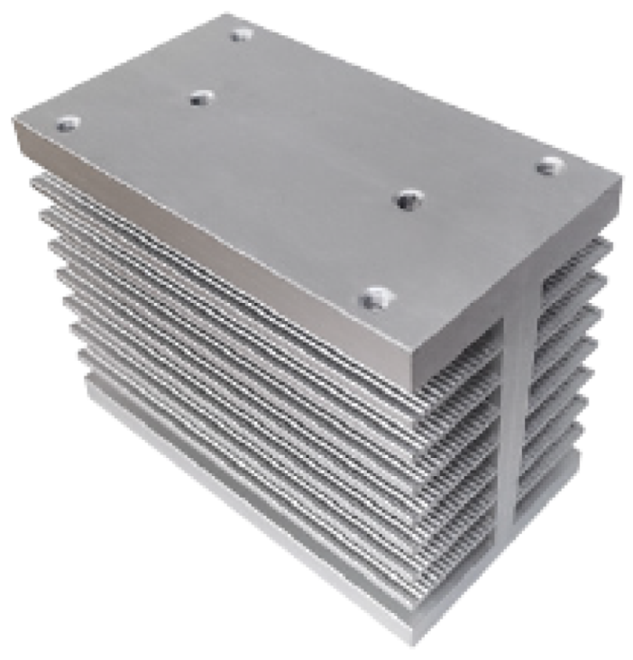
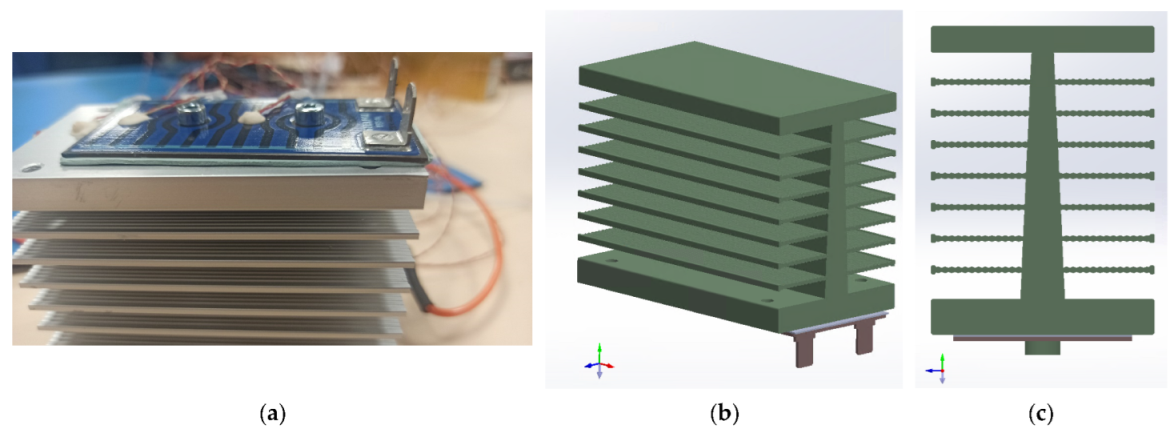
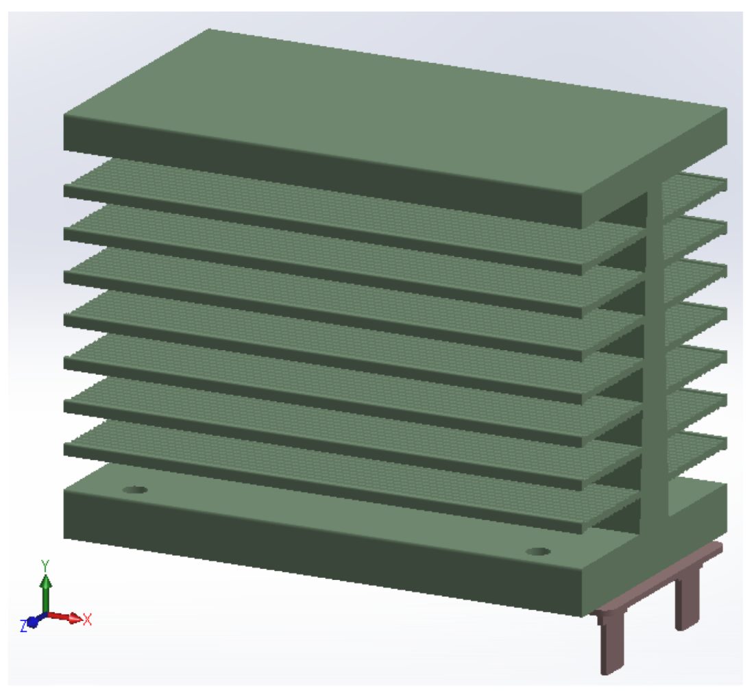
The heat sink used for cooling the heating element is the Relpol RH17A [44]. It is an aluminum heat sink with a 350 g weight. It has an anodized grey color, which means it also has a higher radiation coefficient compared to shiny aluminum. An isometric view of the heat sink can be seen in Figure 2.
It measures 90 mm in length and 50 mm in width, which is more than the surface of the heating element, and 69 mm in height. The fins have a wave-like surface geometry to increase the total surface area. It also has a central rib from the base of the heat sink to transfer the heat from the base to the top of the heat sink, then to each fin and to improve the cooling.
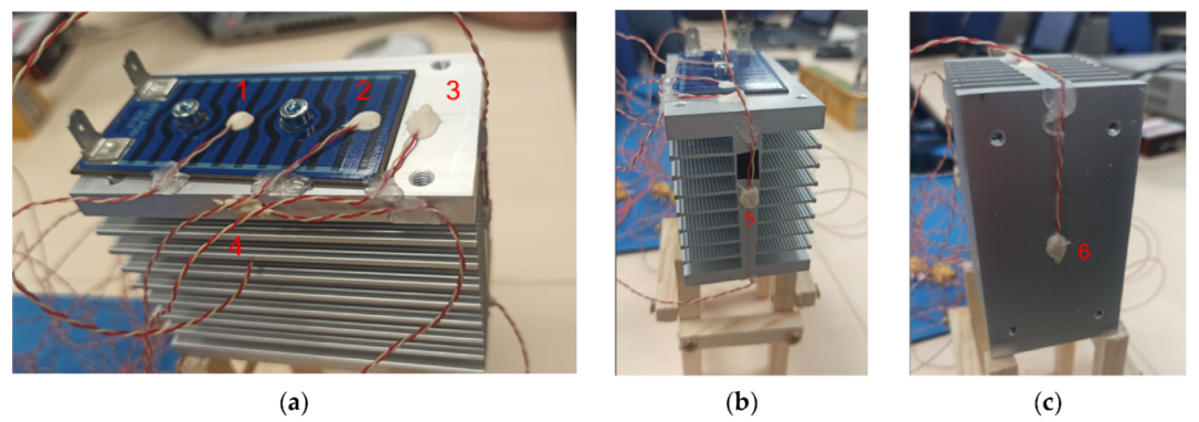
To measure the temperature, RS Pro Type K thermocouples are used. The thermocouples are attached to the thick film heater and heat sink using a ceramic glue. The effect of the ceramic glue on measuring was not evaluated; therefore, the error generated by this type of clamping is unknown. Seven thermocouples are used to measure the temperature as follows: two thermocouples on the thick film heater body (number 1 and 2), four thermocouples placed on the heat sink (number 3 to 6), and one thermocouple placed away from the heater to measure the ambient temperature. An overview of the thermocouple’s placement can be seen in Table 1, and the exact position of the thermocouples on the heat source and heat sink can be seen in Figure 3.
A power supply is used to supply current to the thick film element and generate heat. To gain the 17 W desired power, the power supply provided 56.7 V and 0.3 A. These values are fixed, and the same values were used for all the tested scenarios.
Figure 3a,b shows the measured assembly with thermocouples placed on it, and in Figure 3c, the assembly has the gravity orientation parallel with the heating element length.
  • Setup 1
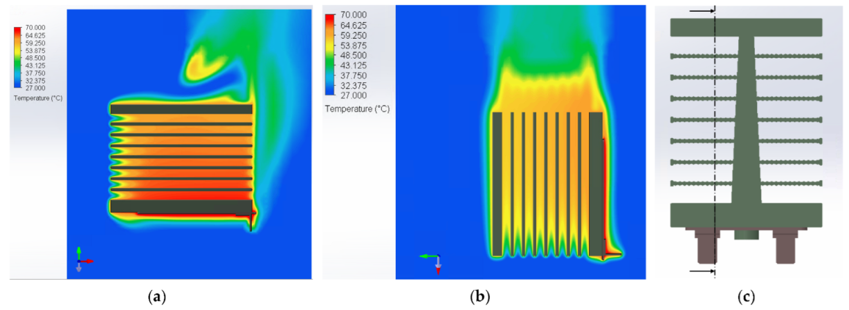
For the first measurement, the thick film heating element is placed under the heat sink. The corners of the heat sink are placed on the wood frame to allow the air natural movement around the heat sink and heat source. The placement of the assembly on the wood frame for Setup 1 measurements can be seen in Figure 4a and the 3D CAD model used for the simulation with the gray arrow that shows gravity orientation perpendicular to the heating element can be seen in Figure 4b.
  • Setup 2
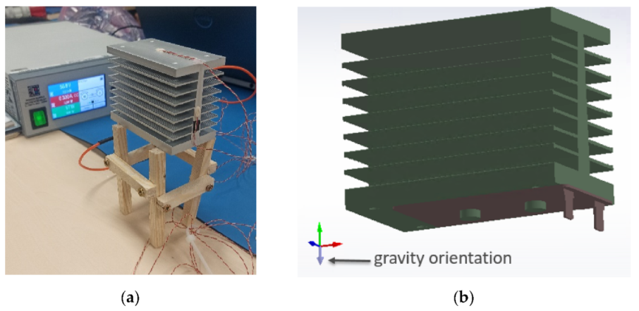
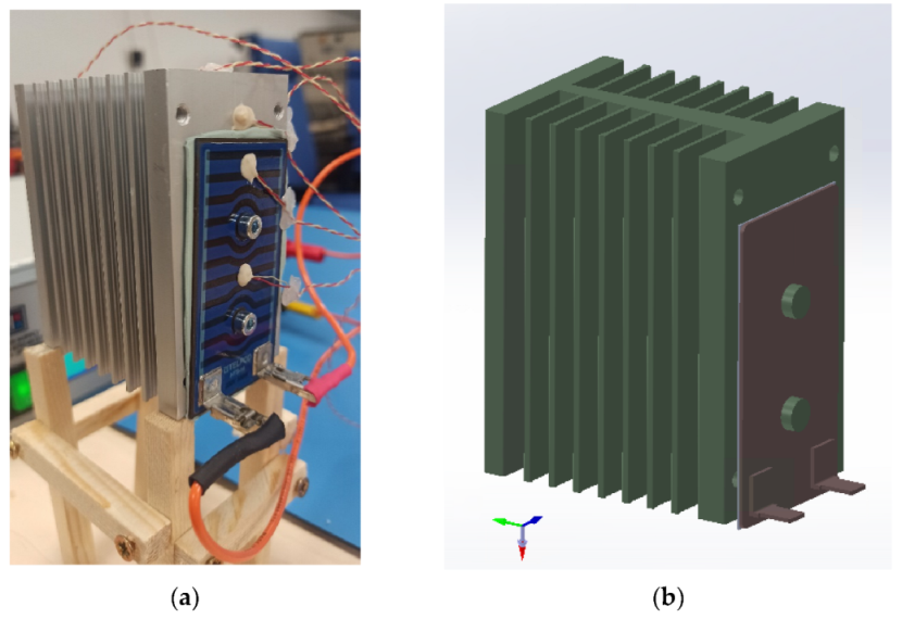
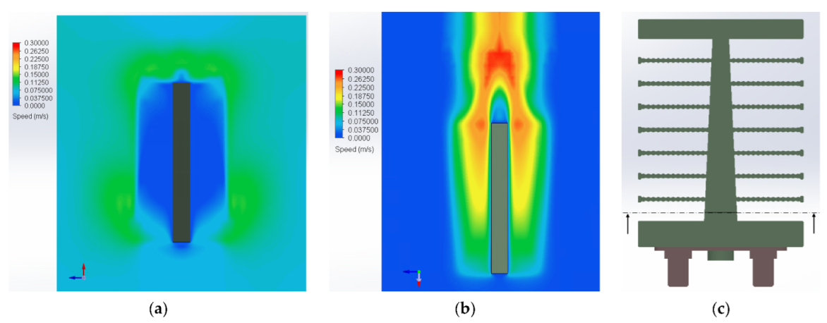
After the thick film heating element reached the steady state temperature, the heat sink was rotated 90° so that the fins are perpendicular to the working surface, as in Figure 5. In this position, the hot air between the heat sink’s fins is expected to rise and start the natural cooling of the components. The assembly was kept in this position until there was no change in the temperatures measured; therefore, the temperature values reached a steady state.
The differences in measured values between the Setup 1 and Setup 2 are due to natural air movement and the improved passive cooling that comes with it. In both setups, the thick film heating element is fixed directly to the heat sink using screws, without any thermal interface material.
  • Setup 3
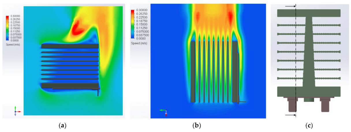
Setup 3 has the same orientation as the first one with the heating element parallel with the working surface. The only difference here is that a thermal interface material is used between the thick film heating element and heat sink, as can be seen in Figure 6. The thermal interface material has the role of improving the thermal transfer between the heat source and heat sink; therefore, improving the cooling.
  • Setup 4
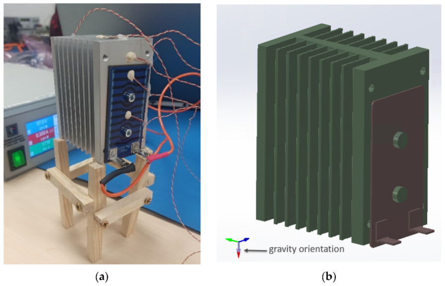
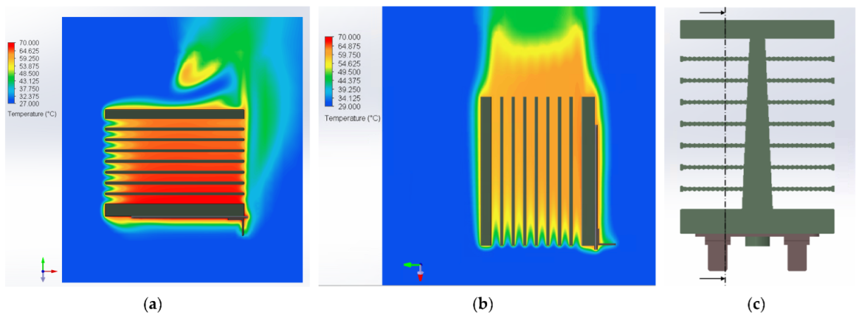
In the fourth setup used for the temperature measurement, the orientation of the assembly is same as in the second setup. The measured and simulated assembly can be seen in Figure 7. The aim is to compare the measured temperatures from this setup with the ones from the third setup and evaluate the impact that changing the orientation has on this assembly.
The aim of the measurement is not to compare the setups with and without thermal interface material; therefore, the first and second setup will not be compared with the third and fourth.
  • Finite element analysis description
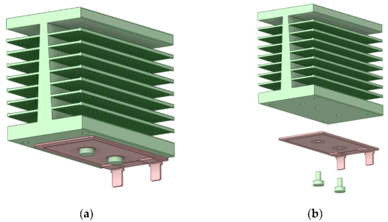
To evaluate the influence of gravity using finite element analysis, a 3D CAD geometry was created to replicate the experimental assembly. The thick film heating element was simplified, using a stainless-steel substrate, and the heat dissipation component was placed on top of it. The heating element was fixed with two screws, also simplified, as shown in Figure 8, since the thread of the screw requires too many computational resources to be simulated for a small thermal transfer influence.
An overview of the gravity vector orientation and use of thermal interface material can be seen in Table 2.
  • Simulation setup
The materials thermal conductivity used for the components are generic material from the Siemens Simcenter Flotherm XT 2021.2 library. The exact thermal conductivity and thermal radiation coefficient of the materials are unknown. The values used are the ones from Table 3 and are assumptions, slightly modified in the calibration process to get similar results as in the real-life test, without significant modifications that may lead to an unrealistic setup.
The thermal radiation coefficient used for the heat sink is 0.8 since the aluminum has an anodized surface, significantly increasing the coefficient, compared to the shiny aluminum. The thick film has an even higher radiation coefficient because it is covered in a lacquer substrate that increases the value of the coefficient.
The model data information are presented in Figure 9. The solution type is kept flowing. Additionally, the heat transfer analysis type is steady state, since the goal is to compare the temperature results after the system reaches thermal equilibrium, and no changes can be seen in the temperature values after that moment.
The turbulence type model is set to laminar and turbulent flow, which allows both types of fluid flows to be calculated in the simulation if needed. The default radiation surface emissivity is set to 0.4 for the components that do not have another thermal radiation coefficient applied particularly for that component.
The equations used by the software to calculate the solution are not visible, therefore, are not available to the user.
Flotherm XT 2021.2 uses a cell-centered finite volume method to obtain conservative approximations of the governing equations on the locally refined rectangular mesh. The governing equations are integrated over a control volume, which is a grid cell, then approximated with the cell centered values of the basic variables.
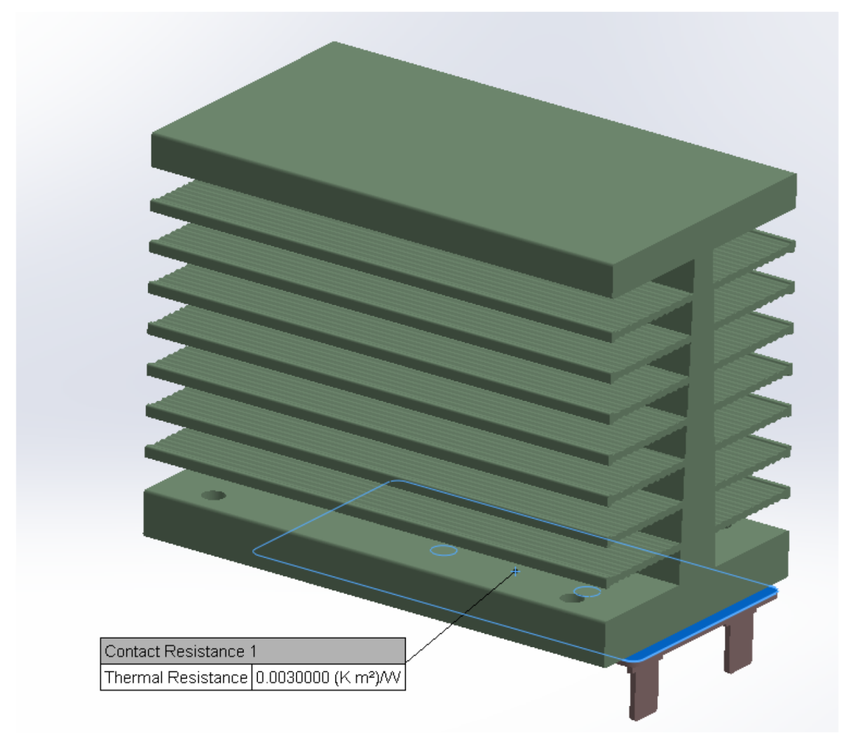
As in Setup 1 and Setup 2, the thick film is fixed directly on the heat sink without using any thermal interface material, a thermal resistance was added between the components, as shown in Figure 10. The value set for the thermal insolence is 0.003 (Km2)/W. As the virtual model the components are in perfect contact, which is ideal, the quantity of heat transferred between the heat source and heat sink was higher.
In Setup 1 and Setup 3, an external velocity value was set in the positive direction of the X axis, represented by the red arrow in Figure 11. This is due to the natural air movement that occurs in the lab due to people moving or equipment fans functioning. The value of the velocity is 0.075 m/s and is an assumption, the actual value of the air speed in the laboratory was not measured.
In Setup 2 and Setup 4, where gravity increases the air movement on the X axis direction due to hot air moving, the external velocity was removed.
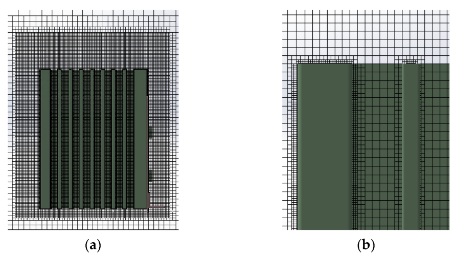
A mesh independent evaluation was completed at the beginning of the investigations. The goal was to reduce the error generated by the size of the mesh elements. An overview of the investigation results can be seen in Table 4. The simulation temperature values between Try 6 and Try 7, measured in the same points, are less than 0.05 °C; therefore, the mesh from Try 7 is used for all four simulations. The total number of mesh elements exceeded 15,000,000.
In Figure 12, the mesh resulted after Try 7 can be seen. A mesh region that includes all the components and surrounding areas is added, mesh refinement is applied on all the solid components, and a Surface Inflation Mesh was applied on the heat sink to reduce the element size in the proximity of the fins.
The first simulation, which replicates Setup 1, was calibrated. Therefore, certain parameters as emissivity, contact resistance and airflow were added until the simulation results were similar to the measured values.
For the rest of the simulation, the same parameters were kept, except the gravity orientation and thermal interface material for Setup 3 and Setup 4.
  • Governing equations
Flotherm XT 2021.2 uses Navier–Stokes Equations for laminar and turbulent fluid flows. The software also uses K-E model for the transport equations for the turbulent kinetic energy and its dissipation rate.
The conservation laws for mass, angular momentum and energy, in the conservation form, can be written as follows:
ρ t + x i ρ u i = 0
ρ u i t + ρ u i u j x j + p x i = T i j + T i j R x j + S i
ρ H t + ρ u i H x i = u j T i j + T i j R + q i x i + p t T i j R U i x j + ρ ε + S i u i + Q H
H = h + u 2 2
where:
u is the fluid velocity;
ρ is the fluid density;
S i is a mass-distributed external force per unit mass:
S i = S i p o r o u s + S i g r a v i t y + S i r o t a t i o n
where:
S i p o r o u s is due to porous media resistance;
S i g r a v i t y is due to buoyancy and = ρ g i ’; where g i is the gravitational acceleration component along the i-th coordinate direction;
S i r o t a t i o n is due to the coordinate system’s rotation;
h is the thermal enthalpy;
Q H is a heat source or sink per unit volume;
T i j is the viscous shear stress tensor;
q i is the diffusive heat flux.
For Newtonian fluids, the viscous shear stress tensor is defined as:
T i j = μ u i x j + u j x i 2 3 δ i j u k x k
Following Boussinesq assumption, the Reynolds-stress tensor has the following form:
T j R = μ t u i x j + u j x i 2 3 δ i j u k x k 2 3 ρ k δ i j
δ i j is the Kronecker delta function (equal to one when I = j, otherwise zero);
μ is the dynamic viscosity coefficient;
μ t is the turbulent eddy viscosity coefficient; and k is the turbulent kinetic energy.
Since Flotherm XT is also a thermal transfer simulation software, it is able to predict that the heat transfer is made through solids and fluids with energy exchanging between them. Heat transfer fluids are defined by Equation (3). Anisotropic heat conductivity in solids is described by the following equation:
ρ e t = λ i T x i x i + Q H
e is the specific internal energy: = c T , where c is specific heat;
Q H is specific heat release (or absorption) per unit volume;
λ i are the eigenvalues of the thermal conductivity tensor.
Heat dissipated through radiation by a surface or radiation source can be defined, for thermal radiation, as:
Q T o u t = ε σ T 4 A + 1 ε Q T i n
ε is the surface emissivity;
σ is the Stefan-Boltzmann constant;
T is the temperature of the surface ( ε σ T 4 is the heat radiated by this surface in accordance with the Stefan-Boltzmann law);
A is the radiative surface area;
Q T i n is the incident thermal radiation arriving at this surface.

3. Results and Discussion

3.1. Measured Temperature Results

Table 5 shows an overview of the measured and simulation temperatures. In the first column, the thermocouple number is shown with the same numbering used when presenting the thermocouple positioning. For each setup, the measured and the simulated temperature values are presented side by side.
In Table 6, a comparison of the measured temperatures of Setup 1 and Setup 2 can be seen, and the difference between the two of them. In Setup 1 and Setup 2, it can be observed that the difference generated by the gravity orientation relative to the heat sink fins is between 7.7 °C and 8.2 °C. On the thick film heater, the temperature dropped in the Setup 2 by 7.9 °C and 7.7 °C in the measured points. On the heat sink, the difference is higher, up to 8.2 °C.
The main reason for the difference is the hot air moving due to lower density and creating a natural movement of the air that enhances convection. Therefore, the thick film heater and the heat sink are locally cooled better.
Additionally, because the thick film heater is cooled better in the first place by improved natural convection, less heat is conducted into the heat sink. This is why the temperature drop in the heat sink body is higher than the temperature drop in the thick film heater.
In Table 7, a similar temperature comparison can be seen for Setup 3 and Setup 4, both with a different ambient temperature (thermocouple 7). The ambient temperature is 0.5 °C higher in Setup 4’s measurement, therefore the measured temperatures are with approximately 0.5 °C higher than would be at the same ambient temperature as in Setup 3.
To evaluate the difference between Setup 3 and Setup 4 as if both were measured at the same ambient temperature, 0.5 °C was subtracted from the Setup 4 measured values. This value of 0.5 °C is the difference between the ambient temperature for Setup 3 and Setup 4. The adjusted temperature values can be seen in Table 8.
In this comparison, where the contact between the heater and heat sink is made using a thermal interface material, the temperatures measured dropped by between 6.2 °C and 6.9 °C. The difference between Setup 3 and Setup 4 is smaller than the difference between Setup 1 and Setup 2 because, in this situation, the thick film heater is cooled more efficiently by using a thermal interface material. Changing the gravity orientation improved the cooling for the same reason as in the first comparison, but the temperatures reached in Setup 3 relative to the ambient temperature are smaller than the temperatures measured in Setup 1.
In both comparisons, we can conclude that the gravity orientation has an impact on passively cooled heat sink elements, and a proper orientation and placement, which will allow the air to move freely around the heat sink fins, will have a positive effect on cooling.

3.2. Results from Finite Element Simulations

Setup 1 simulation was calibrated until the simulation temperatures reached almost the same temperatures as the measured values for similar areas. The simulated temperature values can be seen in Table 9. Therefore, the difference between the simulated Setup 1 and simulated Setup 2 can be compared with the difference between the measured values for the same setups. In this case, the difference in temperatures is between 4.8 °C and 5.4 °C.
For the measured values, where the difference between setups is between 7.7 °C and 8.2 °C, we can say that the effect of the gravity orientation is less precisely observed in the simulation. This difference can be caused by a higher calculation error of the simulation software. The difference between the measured and simulated temperatures for Setup 2 are between 1.2 °C and 3.5 °C, which is very pleasing and useful result for the usual simulation purposes in the industry.

3.2.1. Setup 1 and Setup 2 Simulation Results Comparison

Figure 13 shows a temperature plot of the assembly for Setup 1 and Setup 2 using the same temperature plot history. It can be seen that in Setup 2 the cooling is improved, since the heat sink temperature is lower.
As expected, the air speed between the fins is higher in Setup 2. A section view plot of the air speed for Setup 1 and Setup 2 can be seen in Figure 14, as well where the section plane is placed.
Since the air velocity has an influence on cooling and air temperature, in Figure 15, the air temperature can be seen for the same section view. The air temperature between the fins in Setup 1 is higher than the air temperature between the fins in Setup 2, reducing the convection and radiation effect.
Another air velocity plane plot for a section view can be seen in Figure 16. One can observe that, in Setup 2, the air velocity increases as the temperature of the air increases, and improves the natural effect of hot air rising.

3.2.2. Setup 3 and Setup 4 Simulation Results Comparison

Simulations were made at an ambient temperature similar to the measurement ambient temperature. The obtained temperature values in simulations for Setup 3 and Setup 4 can be seen in Table 10. Since, for Setup 3 and Setup 4, the ambient temperature is different, a temperature adjustment was completed to make a proper comparison between the simulations.
Since for Setup 3 and Setup 4 the ambient temperature is different, a temperature adjustment was completed to make a proper comparison between the simulations. The adjusted values, with 0.8 °C subtracted from the Setup 4 temperature values, can be seen in Table 11. The value of 0.8 °C is the difference between the ambient temperature for Setup 3 and Setup 4.
The difference between the temperature values from the simulation of Setup 3 and Setup 4 is between 4.9 °C and 5.5 °C. Compared with the measured values for the same setups, where the difference is between 6.2 °C and 6.9 °C, one can say that the simulations are more precise and reliable than the previous case.
The similarity with the previous case is that the temperature reduction in simulation on the heat sink is smaller than the temperature reduction in the heat sink in the real-life measurements. Therefore, we can conclude, as in the previous case, that the heat transfer from the heat sink to the ambient may be the higher source of error in the simulation.
The difference between the measured and simulated temperature values for Setup 3 and Setup 4 are up to 2.2 °C, which makes the simulation reliable and useful to predict the thermal behavior of the assembly.
As in the previous visual evaluation, when comparing temperature plot of Setup 3 with the one of Setup 4, we can clearly see that, for the same plot history, the components in Setup 4 are cooled better, as in Figure 17.
For an air velocity comparison between the fins, which can be seen in Figure 18, the same position for the section view was used as before. It can be also seen that gravity has an influence on air velocity.
Figure 19 is a good example of why heat sink orientation is important because it can be easily seen that the hot air passes through the fins and is released in the ambient air, cooling the heat sink fins. Even if Setup 3 has an air velocity on X axis, the velocity values are too slow to have a significant influence and force the air to pass through the fins.
Figure 20 shows us again that gravity increases the hot air velocity between the fins.

4. Conclusions

The investigation focused first on the influence of gravity orientation, and second, on the reliability of finite element analysis in predicting the temperature values of passive cooled heat sinks.
Heat sink fins orientation relative to the gravity vector has an impact in passively cooling the heat sink. During performed experiments, in various setups, measured temperatures were reduced up to 8.2 °C by changing the gravity orientation. The temperature measurement during the experiments was carried out in seven points using thermocouples, distributed on the heat sink structure, and allowed the evaluation of the temperature between the two experimental setups and later the calibration of the analysis with finite elements. Gravity improves the air natural movement between the heat sink fins and thereby increases the air speed, resulting in a reduced heat sink and heat source temperature.
Gravity should be taken into consideration when designing a passively cooled system.
In addition, finite element analysis proved to be a reliable method of predicting the thermal behavior of the assemblies. The simulated temperature values are similar to the measured ones, considering that there are multiple possible error sources. An advantage of the simulation is that it is easier to have an overview of the air movement and its role in cooling the heat sink, also allows faster evaluation of designed structure, especially when the changes to the designed part are incremental.

Author Contributions

Conceptualization, G.-G.C.; methodology, G.-G.C. and D.F.C.; software, A.V.S.; validation, G.-G.C., C.G.D. and P.V.; formal analysis, G.-G.C.; investigation, G.-G.C. and C.G.D.; resources, P.V. and D.F.C.; data curation, C.G.D.; writing—original draft preparation, G.-G.C.; writing—review and editing, G.-G.C., C.G.D. and A.V.S.; visualization, D.F.C.; supervision, C.G.D.; project administration, G.-G.C.; funding acquisition, G.-G.C. All authors have read and agreed to the published version of the manuscript.

Funding

This paper was financially supported by the Project “Network of excellence in applied research and innovation for doctoral and postdoctoral programs/InoHubDoc”, Gheorghe Asachi Technical University of Iasi, Iași, Romania, project co-funded by the European Social Fund financing agreement no. POCU/993/6/13/153437.

Data Availability Statement

The data presented in this study are available on request from the corresponding author.

Acknowledgments

We want to thank Preh Romania for letting us use the testing and measurement equipment.

Conflicts of Interest

The authors declare no conflict of interest. The funders had no role in the design of the study; in the collection, analyses, or interpretation of data; in the writing of the manuscript; or in the decision to publish the results.

References

  1. Merrikh, A.A. Compact thermal modeling methodology for predicting skin temperature of passively cooled devices. Appl. Therm. Eng. 2015, 85, 287–296. [Google Scholar] [CrossRef]
  2. Moore, A.L.; Shi, L. Emerging challenges and materials for thermal management of electronics. Mater. Today 2014, 17, 163–174. [Google Scholar] [CrossRef]
  3. Khetib, Y.; Sedraoui, K.; Melaibari, A.A.; Alzaied, A.; Alsulami, R.; Sharifpur, M. Heat transfer and pressure drop in turbulent nanofluid flow in a pin-fin heat sink: Fin and nanoparticles shape effects. Case Stud. Therm. Eng. 2021, 28, 101378. [Google Scholar] [CrossRef]
  4. Abbas, A.; Muneeshwaran, M.; Wang, C.C. Performance of displaced fin heatsink in natural convection subject to upward and downward arrangement. Int. J. Therm. Sci. 2021, 162, 106797. [Google Scholar] [CrossRef]
  5. Quitadamo, M.V.; Piumatti, D.; Raviola, E.; Fiori, F.; Reorda, M.S. A new technique to check the correct mounting of the power module heatsinks. Microelectron. Reliab. 2022, 128, 114416. [Google Scholar] [CrossRef]
  6. Dusmez, S.; Duran, H.; Akin, B. Remaining useful lifetime estimation for thermally stressed power MOSFETS based on on-state resistance variation. IEEE Trans. Ind. Appl. 2016, 52, 2554–2563. [Google Scholar] [CrossRef]
  7. Russo, S.; Bazzano, G.; Cavallaro, D.; Sitta, A.; Calabretta, M. Thermal analysis approach for predicting power device lifetime. IEEE Trans. Device Mater. Reliab. 2019, 19, 159–163. [Google Scholar] [CrossRef]
  8. Zhang, J.; Sadiqbatcha, S.; Chen, L.; Thi, C.; Sachdeva, S.; Amrouch, H.; Tan, S.X.-D. Hot-spot aware thermoelectric array based cooling for multicore processors. Integration 2023, 89, 73–82. [Google Scholar] [CrossRef]
  9. El Ghandouri, I.; El Maakoul, A.; Saadeddine, S.; Meziane, M.; Dhriss, I. Comparison of thermal performance of plate and corrugated fin heatsinks with a modified base under free convection. Mater. Today Proc. 2022, 66, 100–108. [Google Scholar] [CrossRef]
  10. Hejri, S.; Malekshah, E.H. Cooling of an electronic processor based on numerical analysis on natural convection and entropy production over a dissipating fin equipped with copper oxide/water nanofluid with Koo-Kleinstreuer-Li model. Therm. Sci. Eng. Prog. 2021, 23, 100916. [Google Scholar] [CrossRef]
  11. Toprak, B.İ.; Oskouei, S.B.; Bayer, Ö.; Solmaz, İ. Experimental and numerical investigation of a novel pipe-network mini channel heatsink. Int. Commun. Heat Mass Transf. 2022, 136, 106212. [Google Scholar] [CrossRef]
  12. Torosyan, K.S.; Sedegov, A.S.; Kuskov, K.V.; Abedi, M.; Arkhipov, D.I.; Kiryukhantsev-Korneev, P.V.; Vorotilo, S.; Moskovskikh, D.O.; Mukasyan, A.S. Reactive, nonreactive, and flash spark plasma sintering of Al2O3/SiC composites—A comparative study. J. Am. Ceram. Soc. 2020, 103, 520–530. [Google Scholar] [CrossRef] [Green Version]
  13. Saini, R.A.; Vohra, M.; Singh, A.; Rabbani, T.; Choudhary, M. Comparative thermal performance evaluation of a heat sink based on geometrical and material amendments: A numerical study. Mater. Today Proc. 2022, 50, 816–822. [Google Scholar] [CrossRef]
  14. Hernandez-Perez, J.G.; Carrillo, J.G.; Bassam, A.; Flota-Banuelos, M.; Patino-Lopez, L.D. A new passive PV heatsink design to reduce efficiency losses: A computational and experimental evaluation. Renew. Energy 2020, 147, 1209–1220. [Google Scholar] [CrossRef]
  15. Zhan, Z.; ElKabbash, M.; Li, Z.; Li, X.; Zhang, J.; Rutledge, J.; Singh, S.; Guo, C. Enhancing thermoelectric output power via radiative cooling with nanoporous alumina. Nano Energy 2019, 65, 104060. [Google Scholar] [CrossRef]
  16. Sajid, M.; Hassan, I.; Rahman, A. An overview of cooling of thermoelectric devices. Renew. Sustain. Energy Rev. 2017, 78, 15–22. [Google Scholar] [CrossRef]
  17. Baudoin, A.; Saury, D.; Boström, C. Optimized distribution of a large number of power electronics components cooled by conjugate turbulent natural convection. Appl. Therm. Eng. 2017, 124, 975–985. [Google Scholar] [CrossRef]
  18. Xie, Y.; Lai, Q.; Guo, P.; Tan, J. Investigating the infrared spectral radiative properties of self-ordered anodic aluminum oxide for passive radiative heat dissipation. Infrared Phys. Technol. 2020, 109, 103438. [Google Scholar] [CrossRef]
  19. Lu, X.; Xu, P.; Wang, H.; Yang, T.; Hou, J. Cooling potential and applications prospects of passive radiative cooling in buildings: The current state-of-the-art. Renew. Sustain. Energy Rev. 2016, 65, 1079–1097. [Google Scholar] [CrossRef]
  20. Refaey, H.A.; Abdelrahman, M.A.; Alharthi, M.A.; Bendoukha, S.; Khan, S.G.; Emam, M. Passive cooling of highly-concentrator triple-junction solar cell using a straight-finned heat sink: An experimental investigation. Case Stud. Therm. Eng. 2022, 40, 102521. [Google Scholar] [CrossRef]
  21. Haque, M.R.; Hridi, T.J.; Haque, M.M. CFD studies on thermal performance augmentation of heat sink using perforated twisted, and grooved pin fins. Int. J. Therm. Sci. 2022, 182, 107832. [Google Scholar] [CrossRef]
  22. Subahan, K.; Siva Reddy, E.; Meenakshi Reddy, R. CFD analysis of pin-fin heat sink used in electronic devices. Int. J. Sci. Technol. Res. 2019, 8, 562–569. [Google Scholar]
  23. Mu, E.Z.; Wu, Z.H.; Wu, Z.M.; Chen, X.; Liu, Y.; Fu, X.C.; Hu, Z.Y. A novel self-powering ultrathin TEG device based on micro/nano emitter for radiative cooling. Nano Energy 2019, 55, 494–500. [Google Scholar] [CrossRef]
  24. Hasanuzzaman, M.; Malek, A.; Islam, M.; Pandey, A.; Rahim, N. Global advancement of cooling technologies for PV systems: A review. Sol. Energy 2016, 137, 25–45. [Google Scholar] [CrossRef]
  25. Liu, Z.; Sun, Q.; Song, Y.; Yang, J.; Chen, X.; Wang, H.; Jiang, Z. High-emissivity composite-oxide fillers for high temperature stable aluminum-chromium phosphate coating. Surf. Coat. Technol. 2018, 349, 885–893. [Google Scholar] [CrossRef]
  26. Taylor, S.; Yang, Y.; Wang, L. Vanadium dioxide based Fabry-Perot emitter for dynamic radiative cooling applications. J. Quant. Spectrosc. Radiat. Transfer. 2017, 197, 76–83. [Google Scholar] [CrossRef]
  27. Sait, H. Cooling a plate lithium-ion battery using a thermoelectric system and evaluating the geometrical impact on the performance of heatsink connected to the system. J. Energy Storage 2022, 52, 104692. [Google Scholar] [CrossRef]
  28. Karthikeyan, K.; Karthikeyan, P.; Baskonus, H.M.; Venkatachalam, K.; Chu, Y.M. Almost sectorial operators on Ψ-Hilfer derivative fractional impulsive integro-differential equations. Math. Methods Appl. Sci. 2021, 45, 8045–8059. [Google Scholar] [CrossRef]
  29. Iqbal, M.A.; Wang, Y.; Miah, M.M.; Osman, M.S. Study on Date–Jimbo–Kashiwara–Miwa equation with conformable derivative dependent on time parameter to find the exact dynamic wave solutions. Fractal Fract. 2022, 6, 4. [Google Scholar] [CrossRef]
  30. Ataei, M.; Sadegh Moghanlou, F.; Noorzadeh, S.; Vajdi, M.; Asl, M.S. Heat transfer and flow characteristics of hybrid Al2O3/TiO2–water nanofluid in a minichannel heat sink. Heat Mass Transf. 2020, 56, 2757–2767. [Google Scholar] [CrossRef]
  31. Liu, X.; Zhang, C.F.; Zhou, J.G.; Xiong, X.; Wang, Y.P. Thermal performance of battery thermal management system using fins to enhance the combination of thermoelectric Cooler and phase change Material. Appl. Energy 2022, 322, 119503. [Google Scholar] [CrossRef]
  32. Liu, X.; Zhang, C.F.; Zhou, J.G.; Xiong, X.; Zhang, C.C.; Wang, Y.P. Numerical simulation of hybrid battery thermal management system combining of thermoelectric cooler and phase change material. Energy Rep. 2022, 8, 1094–1102. [Google Scholar] [CrossRef]
  33. Chen, D.; Xiao, L.; Yan, W.; Li, Y.; Guo, T. A heat dissipation design strategy based on computational fluid dynamics analysis method for shunt active power filter. Energy Rep. 2022, 8, 229–238. [Google Scholar] [CrossRef]
  34. Liu, H.; Yu, J.; Wang, R. Model predictive control of portable electronic devices under skin temperature constraints. Energy 2022, 260, 125185. [Google Scholar] [CrossRef]
  35. Yang, H.; Zhang, J.; Xia, G.; Zhao, H.; Song, X. Analysis of air-cooling module with multi-TEC. Int. Commun. Heat Mass Transf. 2022, 134, 106041. [Google Scholar] [CrossRef]
  36. Krane, P.; Gonzalez, C.D.; Lozano, F.; Paniagua, G.; Marconnet, A. Sensitivity coefficient-based inverse heat conduction method for identifying hot spots in electronics packages: A comparison of grid-refinement methods. J. Electron. Packag. Trans. ASME 2022, 144, 011008. [Google Scholar] [CrossRef]
  37. Jiang, R.; Zhong, C.; Li, C.; Li, Y.; Peng, X.; Lu, J.; Sun, R. The influence of external factors on the temperature distribution of flip-chip package–Comparative Analysis between Flotherm and Abaqus. In Proceedings of the 23rd International Conference on Electronic Packaging Technology, Dalian, China, 10–13 August 2022; p. 182631. [Google Scholar]
  38. Chen, P.; Tsai, R. Simulation Study On The Heat Transfer Rate Of Thermal Modules With Different Fin Array Modes. J. Chin. Soc. Mech. Eng. 2021, 42, 255–261. [Google Scholar]
  39. Seetharaman, R.; Anitha, D. Analysis of reliability based on thermal cycle and aging effect in electron devices. Pramana-J. Phys. 2021, 95, 55. [Google Scholar] [CrossRef]
  40. Guggari, S.I. Analysis of Thermal Performance Metrics-Application to CPU Cooling in HPC Servers, IEEE Transactions on Components. Packag. Manuf. Technol. 2021, 11, 222–232. [Google Scholar] [CrossRef]
  41. Kim, J.K. Thermal characterization of automotive power module with SHERPA. In Proceedings of the 2021 IEEE 23rd Electronics Packaging Technology Conference, Virtual, 1–3 December 2021; pp. 479–482. [Google Scholar]
  42. Goswami, A.; Guggari, S. Thermal Characterization of Battery Cold Plates. In Proceedings of the 2021 IEEE 23rd Electronics Packaging Technology Conference, Virtual, 1–3 December 2021; pp. 488–492. [Google Scholar]
  43. Telpod. Product Information Telpod HTS-16. Available online: https://www.telpod.eu/en/_files/ugd/b5b7b4_213029500ebd4cee8096ac38f280e67b.pdf (accessed on 13 January 2023).
  44. TME. Product Information Relpol RH17A. Available online: https://www.tme.eu/Document/629098d34a5e4ce9cf4f46f359a8a36e/RH04A-F220AC.PDF (accessed on 13 January 2023).
Figure 1. Telpod HTS-16-230-300-3/6.3 thick film heating element dimensions expressed in mm.
Processes 11 00896 g001
Figure 2. Relpol RH17A heat sink.
Processes 11 00896 g002
Figure 3. (a) Top view of the assembly and position of thermocouples 1 to 4; (b) Side view of the measured assembly and position of thermocouple 5; (c) Bottom view of the simulation assembly and position of thermocouple 6.
Processes 11 00896 g003
Figure 4. (a) Measurement of Setup 1; (b) Simulated model of Setup 1 and gravity orientation.
Processes 11 00896 g004
Figure 5. (a) Measurement of Setup 2; (b) Simulated model of Setup 2 and gravity orientation.
Processes 11 00896 g005
Figure 6. (a) Measurement of Setup 3 with thermal pad added; (b) Isometric view of simulated model of Setup 3 and gravity orientation; (c) Side view of Setup 3.
Processes 11 00896 g006
Figure 7. (a) Measurement of Setup 4; (b) Simulated model of Setup 4 and gravity orientation.
Processes 11 00896 g007
Figure 8. (a) Simulated geometry; (b) Exploded view of the simulated geometry.
Processes 11 00896 g008
Figure 9. Model Data used in the FEA simulation.
Processes 11 00896 g009
Figure 10. Thermal resistance between thick film heating element and heat sink.
Processes 11 00896 g010
Figure 11. Velocity of 0.075 m/s on X axis, marked with the red arrow.
Processes 11 00896 g011
Figure 12. (a) Global mesh on plane plot; (b) Mesh detail in heatsink fins proximity.
Processes 11 00896 g012
Figure 13. (a) Temperature plot of Setup 1 simulation; (b) Temperature plot of Setup 2 simulation.
Processes 11 00896 g013
Figure 14. (a) Air velocity of Setup 1—section view; (b) Air velocity of Setup 2—section view; (c) Section plane.
Processes 11 00896 g014
Figure 15. (a) Air temperature of Setup 1—section view; (b) Air temperature of Setup 2—section view; (c) Section plane.
Processes 11 00896 g015
Figure 16. (a) Air velocity of Setup 1—section view; (b) Air velocity of Setup 2—section view; (c) Section plane.
Processes 11 00896 g016
Figure 17. (a) Temperature plot of Setup 3 simulation; (b) Temperature plot of Setup 4 simulation.
Processes 11 00896 g017
Figure 18. (a) Air velocity of Setup 3—section view; (b) Air velocity of Setup 4—section view; (c) Section plane.
Processes 11 00896 g018
Figure 19. (a) Air temperature of Setup 3—section view; (b) Air temperature of Setup 4—section view; (c) Section plane.
Processes 11 00896 g019
Figure 20. (a) Air velocity of Setup 3—section view; (b) Air velocity of Setup 4—section view; (c) Section plane.
Processes 11 00896 g020
Table 1. Thermocouple positions.
Thermocouple NumberThermocouple Placement PartDetails
1Thick film heating elementMiddle of the thick film
2Thick film heating elementSide of the thick film; opposite side of the current connections
3Heat sinkBottom area, next to the thick film
4Heat sinkSide area of the heat sink, next to the thick film middle
5Heat sinkSide middle area of the heat sink; central column;
6Heat sinkTop of the heat sink, center area
7Ambient
Table 2. Setup overview.
Setup NameGravity Vector orientation Relative to Heatsink finsThermal Interface Material
Setup 1PerpendicularNo
Setup 2ParallelNo
Setup 3PerpendicularYes
Setup 4ParallelYes
Table 3. Material definition used in simulations.
ComponentMaterial UsedThermal Conductivity [W/(mK)]Thermal Radiation
Coefficient
Heat sinkAnodized aluminum1400.8
ScrewsSteel51.90.8
Thick film substrateStainless Steel16.30.9
Thick film–heat generatorCopper3950.9
Table 4. Simulations temperatures in mesh independent model evaluation.
Try 1Try 2Try 3Try 4Try 5Try 6Try 7
No. of mesh elements181,644257,0321,761,4821,795,3182,332,3498,531,62815,247,324
T.C. numberTemperature [°C]
163.9764.0364.7464.7864.9165.1965.17
263.563.5464.2464.364.4364.7264.7
361.661.6362.3462.3862.5262.8162.77
462.7862.8263.5663.663.7364.0263.98
559.8659.960.5460.5760.726160.97
657.8657.958.5358.5658.6858.9758.94
Table 5. Temperature results overview: measurements and simulations.
Setup 1Setup 2Setup 3Setup 4
Thermocouple NumberMeasurement [°C]Simulation [°C]Measurement [°C]Simulation [°C]Measurement [°C]Simulation [°C]Measurement [°C]Simulation
180.480.972.575.772.069.965.665.2
281.880.374.275.369.569.263.664.7
365.165.557.460.566.367.160.662.8
466.266.858.061.567.568.661.564.0
563.963.456.058.665.165.159.561.0
662.562.154.456.763.963.757.758.9
727.327.027.327.028.228.228.729.0
Table 6. Temperature measurements for Setup 1 and Setup 2.
Setup 1Setup 2Delta T
Thermocouple NumberMeasurement [°C]Measurement [°C]S1–S2
180.472.57.9
281.874.27.7
365.157.47.7
466.258.08.2
563.956.07.9
662.554.48.0
Table 7. Temperature measurements for Setup 3 and Setup 4.
Setup 3Setup 4Delta T
Thermocouple NumberMeasurement [°C]Measurement [°C]S3–S4
172.065.66.4
269.563.65.9
366.360.65.7
467.561.56.0
565.159.55.6
663.957.76.2
728.228.7-0.5
Table 8. Temperature measurements for Setup 3 and Setup 4 with adjusted temperatures for Setup 4.
Setup 3Setup 4Delta T
Thermocouple NumberMeasurement [°C]Measurement [°C]S3–S4
172.065.16.9
269.563.16.4
366.360.16.2
467.561.06.5
565.159.06.2
663.957.16.8
28.228.20.0
Table 9. Simulations temperature for Setup 1 and Setup 2.
Setup 1Setup 2Delta T
Thermocouple NumberSimulation [°C]Simulation [°C]S1–S2
180.975.75.2
280.375.34.9
365.560.55.0
466.861.55.3
563.458.64.8
662.156.75.4
727.027.00.0
Table 10. Simulations temperature for Setup 3 and Setup 4.
Setup 3Setup 4Delta T
Thermocouple NumberSimulationSimulationS3–S4
169.965.24.7
269.264.74.5
367.162.84.3
468.664.04.6
565.161.04.1
663.758.94.7
728.229.0-0.8
Table 11. Simulations temperature for Setup 3 and Setup 4 with adjusted temperatures for Setup 4.
Setup 3Setup 4Delta T
Thermocouple NumberSimulationSimulationS3–S4
169.964.45.5
269.263.95.3
367.162.05.1
468.663.25.4
565.160.24.9
663.758.15.5
728.228.20.0
Disclaimer/Publisher’s Note: The statements, opinions and data contained in all publications are solely those of the individual author(s) and contributor(s) and not of MDPI and/or the editor(s). MDPI and/or the editor(s) disclaim responsibility for any injury to people or property resulting from any ideas, methods, instructions or products referred to in the content.

