
Structure Size Optimization and Internal Flow Field Analysis of a New Jet Pump Based on the Taguchi Method and Numerical Simulation
 ,
,
Abstract
:1. Introduction
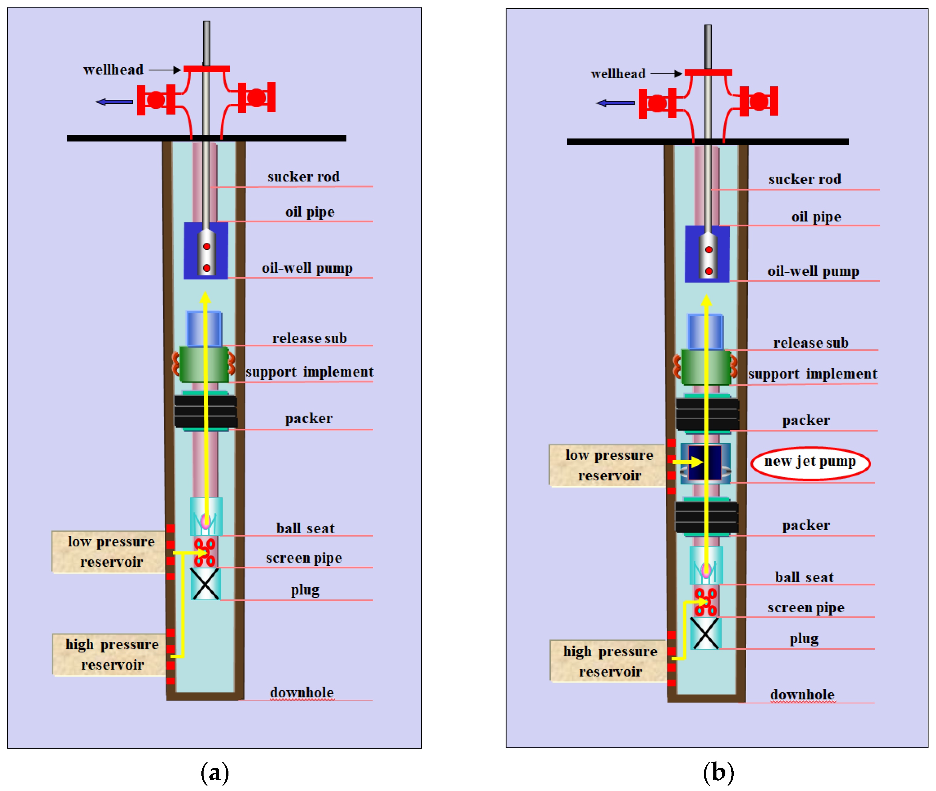
2. The Structure and Working Principle of the New Jet Pump
3. Establishment of Calculation Method and Simulation Model
3.1. Basic Governing Equations of Fluids
3.2. Choice of Turbulence Model
3.3. Calculation Formula of Pump Efficiency
3.4. Basic Characteristic Equation of Jet Pump
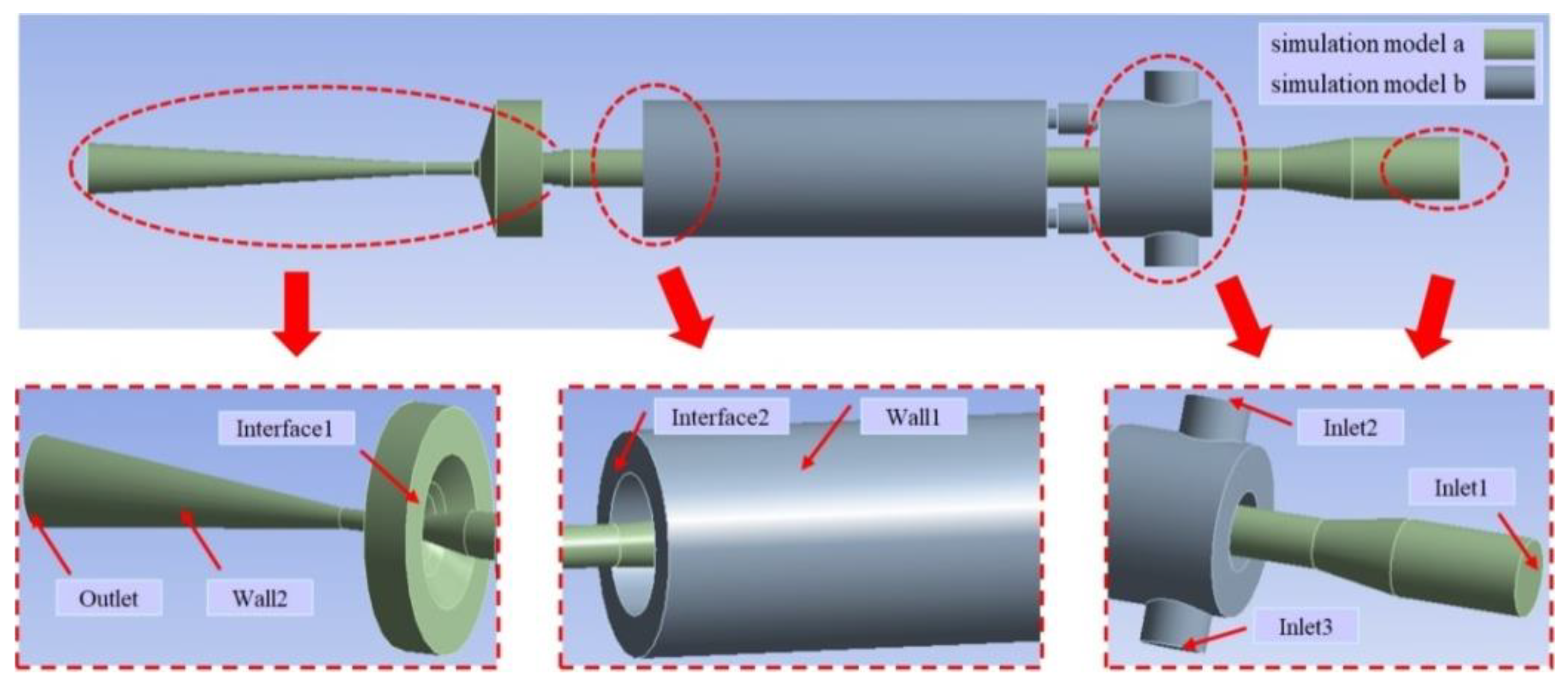
3.5. Establishment of a Simulation Model of the New Jet Pump
4. Meshing and Convergence Analysis of Simulation Model
5. Analysis of Influencing Factors of Pump Efficiency
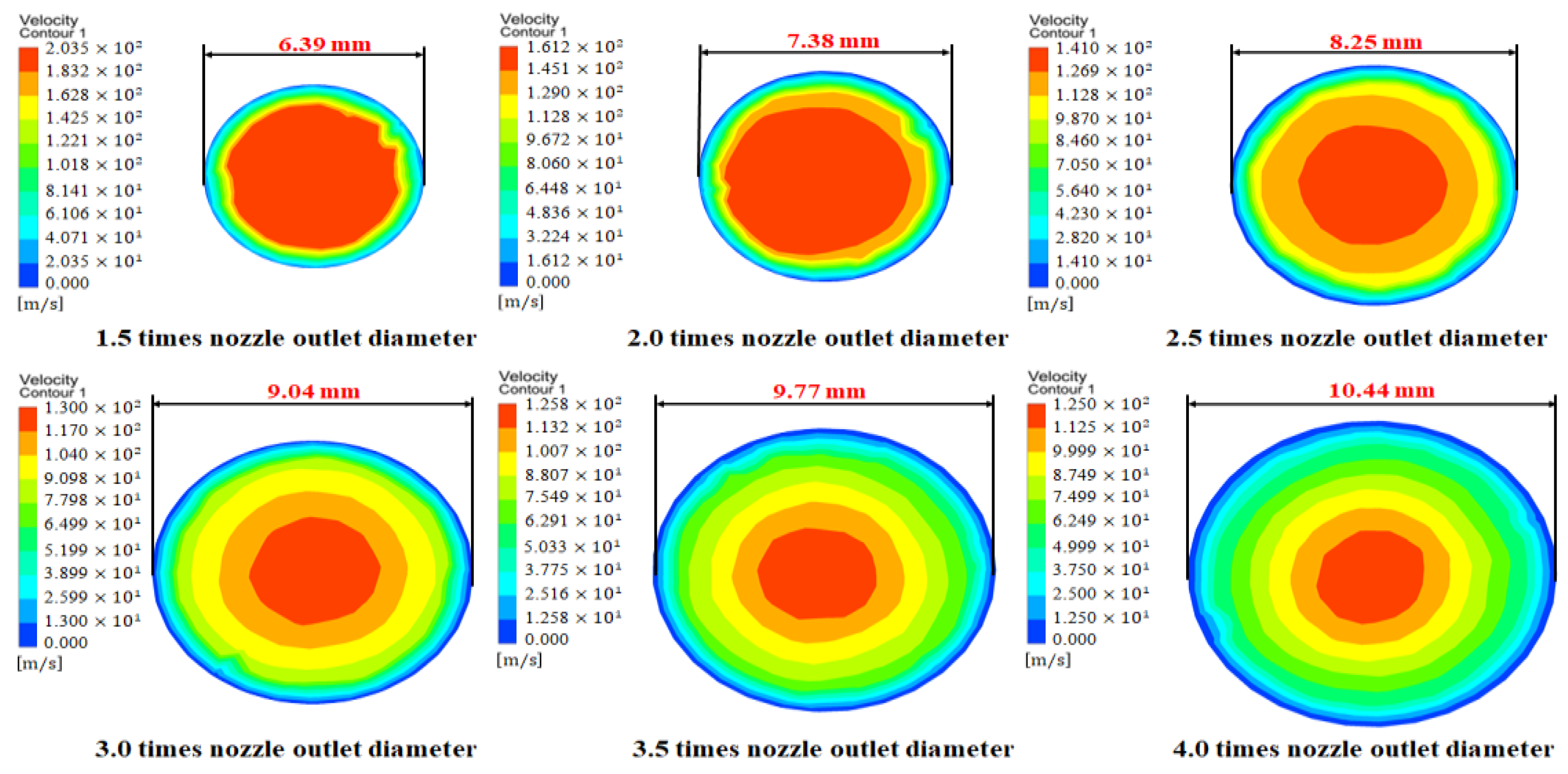
5.1. Effect of the Throat–Nozzle Distance on Pump Efficiency
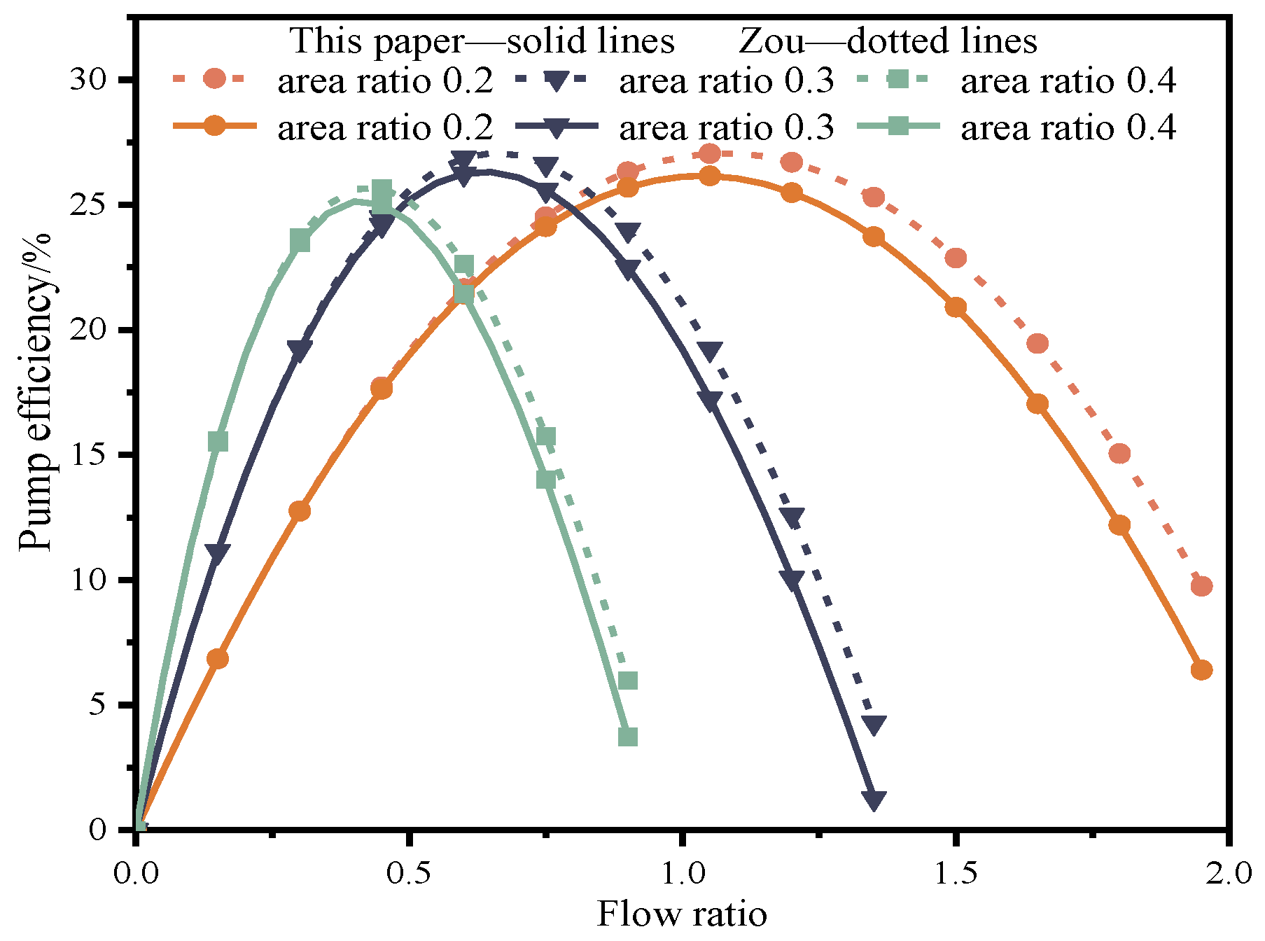
5.2. Effect of Area Ratio on Pump Efficiency
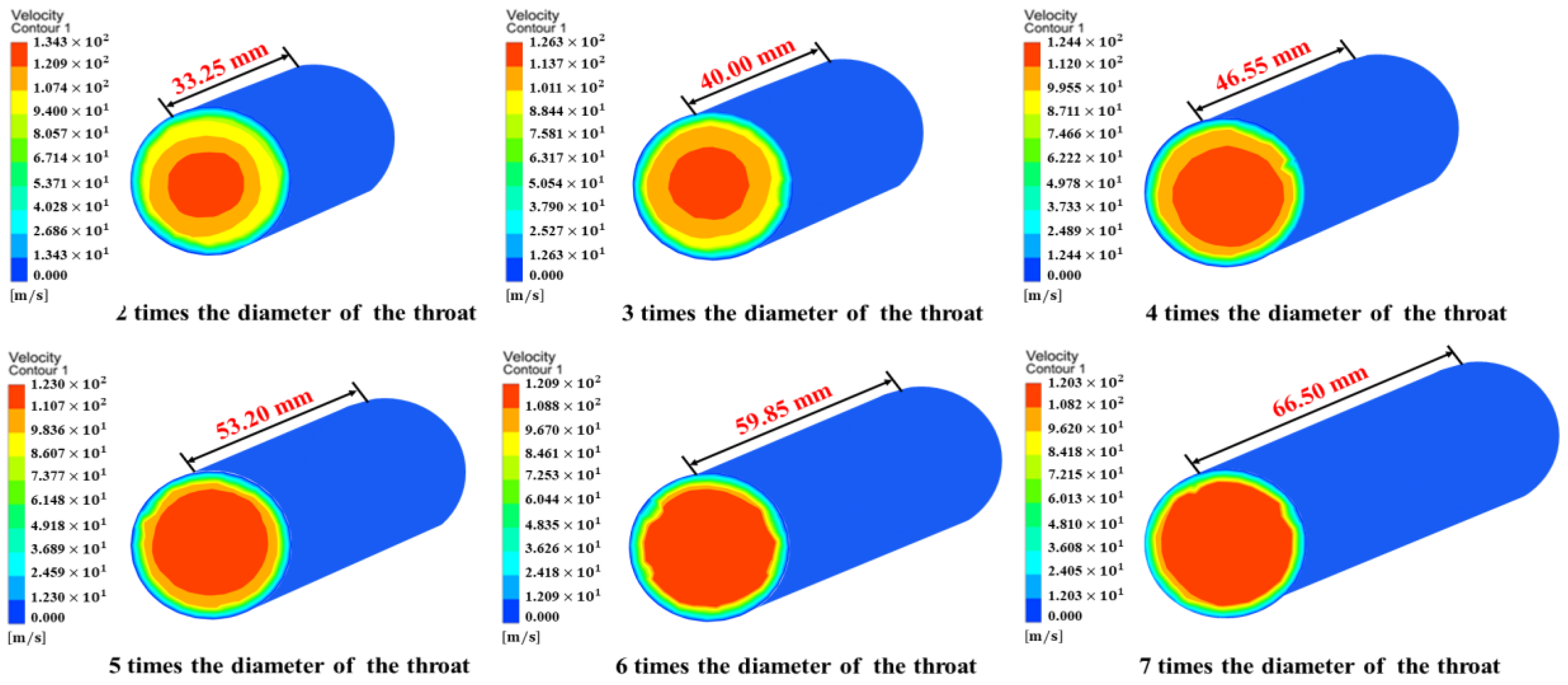
5.3. Effect of the Throat Length–Diameter Ratio on Pump Efficiency
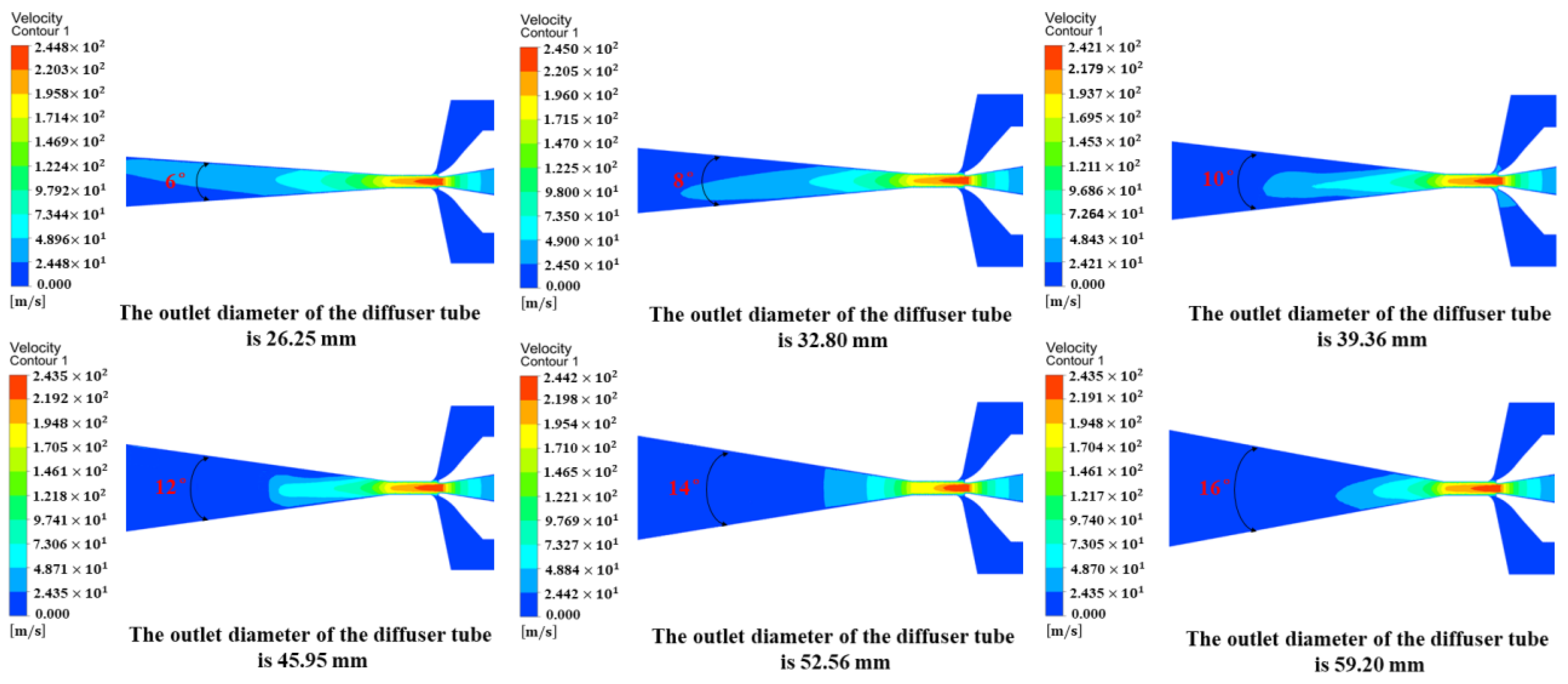
5.4. Effect of Angle of the Diffuser Tube on Pump Efficiency
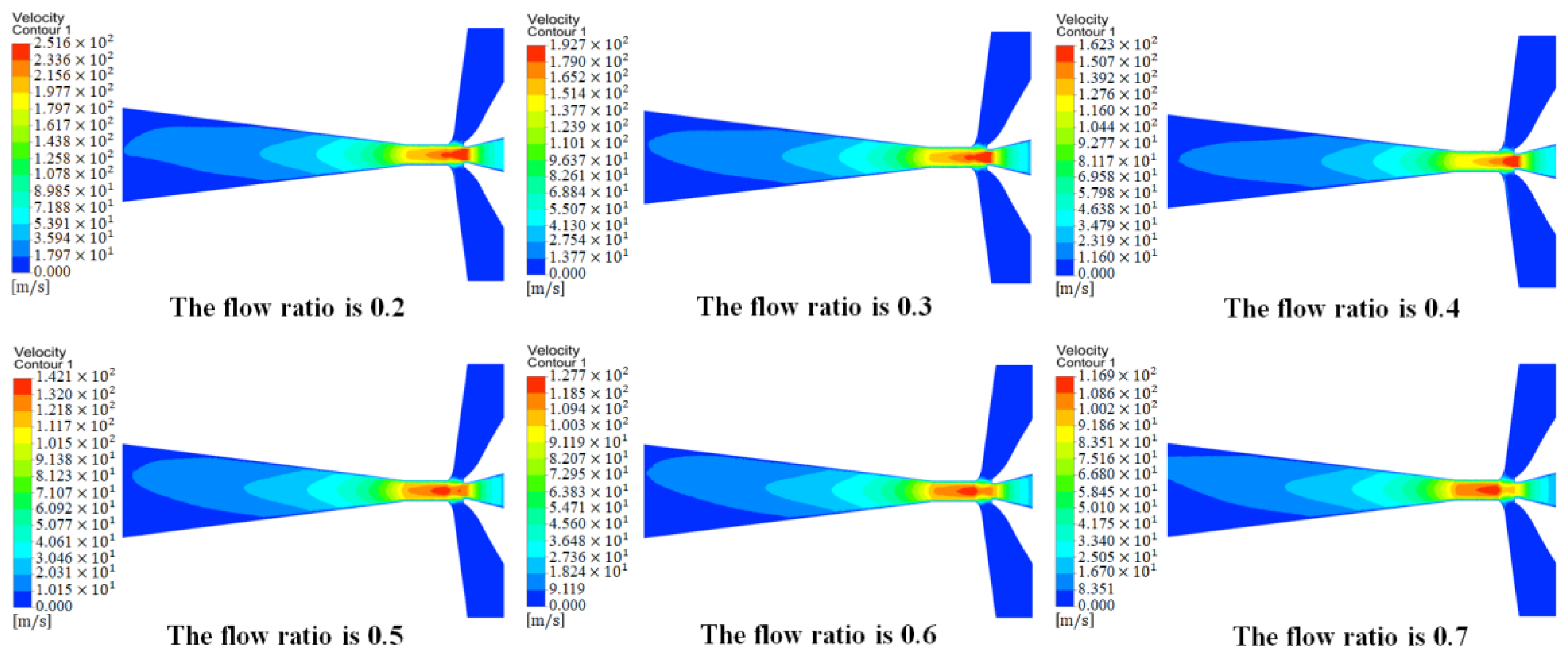
5.5. Effect of the Flow Rate on the Pump Efficiency
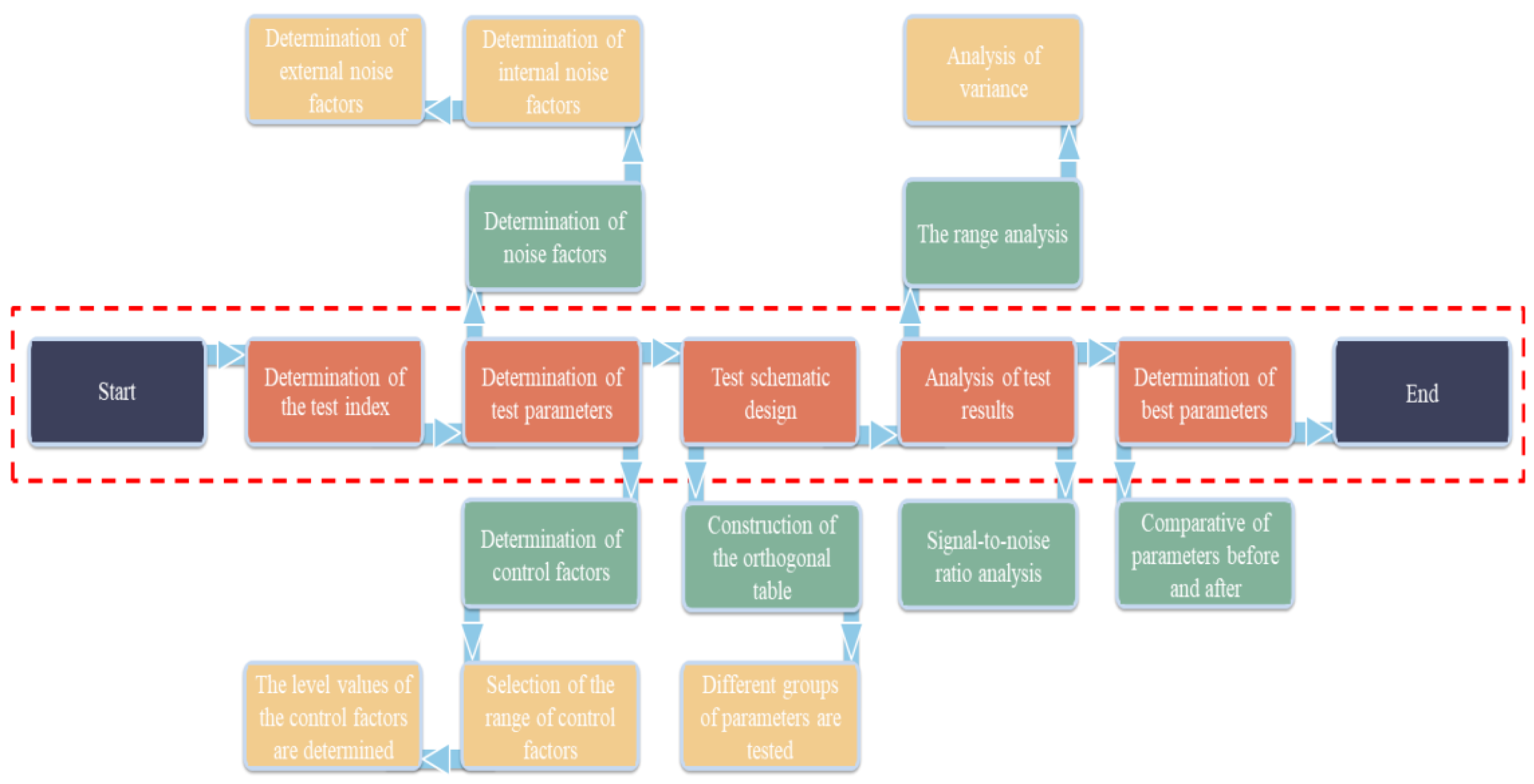
6. Structure Size Analysis of a New Jet Pump Based on the Taguchi Method
6.1. Determination of the Test Index and Control Factors
6.2. The Range and Level of the Control Factors
6.3. Determination of Noise Factors
6.4. Construction of Orthogonal Tables and Orthogonal Tests
6.5. Signal-to-Noise Ratio Analysis of Test Results
6.6. Range Analysis of Test Results
6.7. Variance Analysis of Test Results
7. Comparative Analysis of the New Jet Pump before and after Optimization
8. Conclusions
- A new type of jet pump was designed to enhance the efficiency of oil recovery in wells in Eastern Shandong, China and to effectively exploit low-energy and low-yield zones. The jet pump simultaneously extracts oil from high- and low-pressure reservoirs by transforming the existing contradiction between layers in the well based on the Venturi jet principle. The method further lowers costs and enhances efficiency compared with traditional oil-recovery methods. Thanks to its simple structure, good practicality, and high reliability, the new jet pump also reduces the risk of underground safety accidents.
- A new equation for the basic characteristics of the new jet pump was derived. A comparison of this new equation with the existing equations verified the correctness of this equation. According to the analysis of the envelope curve of the performance (drawn in the 2016 version of MATLAB using the derived equation of basic characteristics) of the jet pump, the density ratio, flow rate ratio, and area ratio had a significant influence on pump efficiency; in addition, as the density ratio gradually increased, both the highest pumping efficiency among different density ratios and the flow ratio corresponding to the highest pumping efficiency gradually decreased.
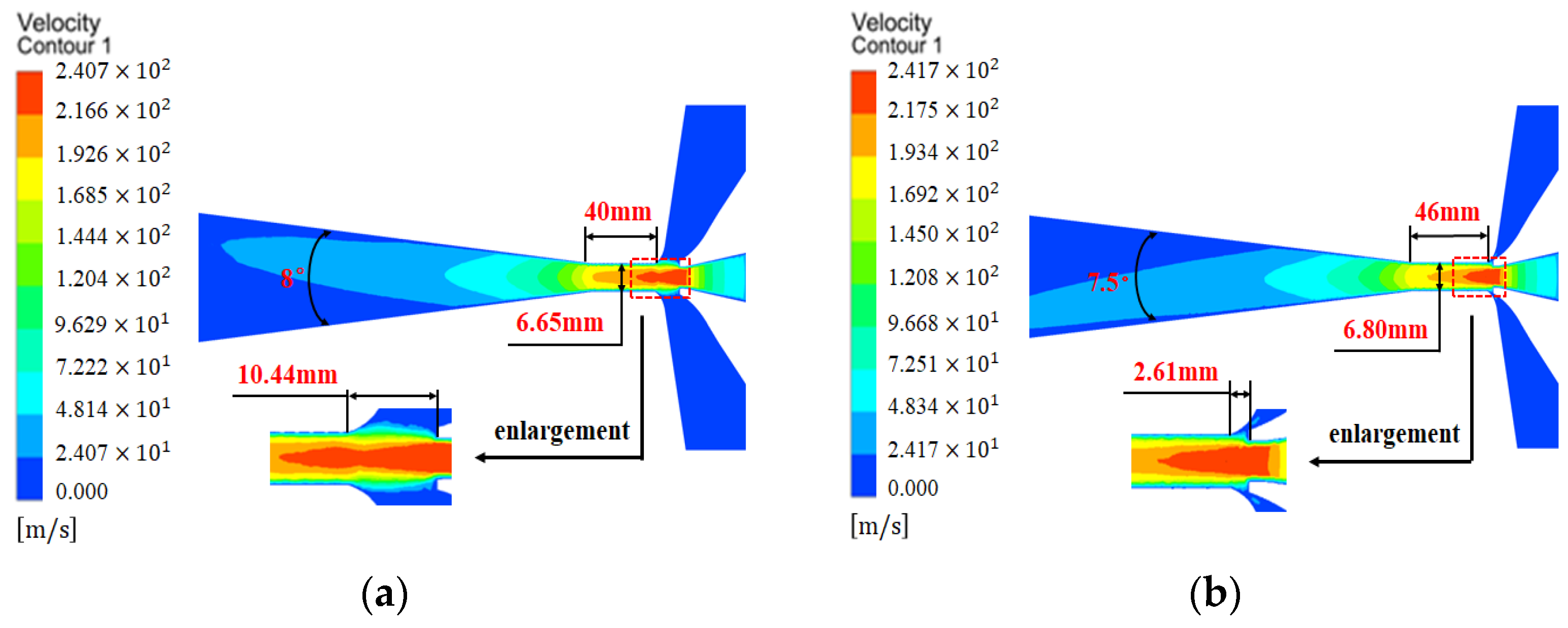
- According to an analysis of the internal flow field of the new jet pump, the increase in the throat–nozzle distance attenuated the flow core area because the effective action distance of the intake fluid being carried became longer due to the power fluid; thus, the velocity of the fluid was significantly reduced before it entered the throat. As the area ratio increased, both the maximum velocity at the throat outlet and the area of the maximum velocity gradually decreased (the reason for this is that as the area ratio gradually increased, the power fluid and the intake fluid carried out a more adequate energy transfer in the throat tube). An increase in the aspect ratio caused the maximum velocity area at the throat outlet to gradually increase (the reason for this is that the contact time between the power fluid and the intake fluid in the throat became longer, and therefore, the two could allow for a more full energy transfer). The increase in the diffuser angle resulted in the velocity distribution area in the diffuser tube not being able to cover the whole cross-section of the diffuser tube (the reason for this is that the velocity of miscible fluids decreased significantly less than the increase in the diffuser angle, which caused the velocity distribution surface in the diffuser tube to not fill the entire diffuser tube section).
- To improve the pumping efficiency of the new jet pump in the extraction of high- and low-pressure reservoirs, its structural dimensions were optimized using the Taguchi method and numerical simulations (this is a new method for optimizing the structure of jet pumps). According to an analysis of the test results using signal-to-noise ratio and range analyses, the factors influencing pumping efficiency are, in descending order, the throat diameter, diffuser angle, throat–nozzle distance, and throat length. The contributions (relative influence on pumping efficiency) of these control factors were then obtained using an ANOVA. The throat diameter had the highest contribution (75.93%), followed by the diffuser angle (9.64%), throat–nozzle distance (9.12%), and throat length (5.31%).
- The efficiency of the new jet pump was optimized with a combination of parameters including a level 1 throat–nozzle distance, a level 2 throat diameter, a level 2 throat length, and a level 3 diffuser angle (i.e., a throat–nozzle distance of 2.62 mm, a throat diameter of 6.8 mm, a throat length of 46 mm, and a diffuser angle of 7.5°). A comparison with the jet pump before optimization indicated that the pump efficiency was increased from 21.81% to 31.26%, further demonstrating a considerable improvement in the performance of the new jet pump.
Author Contributions
Funding
Data Availability Statement
Conflicts of Interest
References
- Wang, H.; Huang, H.; Bi, W.; Ji, G.; Zhou, B.; Zhuo, L. Deep and ultra-deep oil and gas well drilling technologies: Progress and prospect. Nat. Gas Ind. B 2022, 9, 141–157. [Google Scholar] [CrossRef]
- Wu, X.; Wan, F.; Chen, Z.; Han, L.; Li, Z. Drilling and completion technologies for deep carbonate rocks in the Sichuan Basin: Practices and prospects. Nat. Gas Ind. B 2020, 7, 547–556. [Google Scholar] [CrossRef]
- Bintarto, B.; Auliya, R.R.; Putra, R.A.M.; Pradipta, A.S.; Kurnia, R.A. Production Data Analysis and Sonolog for Determining Artificial Lift Design and Well Characteristic. J. Pet. Geotherm. Technol. 2020, 1, 28–35. [Google Scholar] [CrossRef]
- Kolawole, O.; Gamadi, T.D.; Bullard, D. Artificial lift system applications in tight formations: The state of knowledge. SPE Prod. Oper. 2020, 35, 422–434. [Google Scholar] [CrossRef]
- Clegg, J.; Bucaram, S.; Hein, N. Recommendations and Comparisons for Selecting Artificial-Lift Methods (includes associated papers 28645 and 29092). J. Pet. Technol. 1993, 45, 1128–1167. [Google Scholar] [CrossRef]
- Holden, J. Fixing the Deep-Well Jet Pump. Midwest Q. 2009, 50, 357–359. [Google Scholar]
- Zou, C.H.; Li, H.; Tang, P.; Xu, D.H. Effect of structural forms on the performance of a jet pump for a deep well jet pump. In Proceedings of the 17th International Conference on Computational Methods and Experimental Measurements, Opatija, Croatia, 5–7 May 2015. [Google Scholar]
- Zhang, H.; Zou, D.; Yang, X.; Mou, J.; Zhou, Q.; Xu, M. Liquid–Gas Jet Pump: A Review. Energies 2022, 15, 6978. [Google Scholar] [CrossRef]
- van der Lingen, T.W. A jet pump design theory. J. Fluids Eng. 1960, 82, 1128–1167. [Google Scholar] [CrossRef]
- Mallela, R.; Chatterjee, D. Numerical investigation of the effect of geometry on the performance of a jet pump. Proc. Inst. Mech. Eng. Part C J. Mech. Eng. Sci. 2011, 225, 1614–1625. [Google Scholar] [CrossRef]
- Lu, H.Y. Theory and Application of Jet Technology; Wuhan University Press: Wuhan, China, 2004. [Google Scholar]
- Reddy, Y.R.; Kar, S. Theory and performance of water jet pump. J. Hydraul. Div. 1968, 94, 1261–1282. [Google Scholar] [CrossRef]
- Cunningham, R.G. Gas compression with the liquid jet pump. J. Fluids Eng. 1974, 96, 203–215. [Google Scholar] [CrossRef]
- Grupping, W.; Coppes, J.L.R.; Groot, J.G. Fundamentals of oil well jet pumping. SPE Prod. Eng. 1988, 3, 9–14. [Google Scholar] [CrossRef]
- Winoto, S.H.; Li, H.; Shah, D.A. Efficiency of jet pumps. J. Hydraul. Eng. 2000, 126, 150–156. [Google Scholar] [CrossRef]
- Wang, C.B. Research on the Jet Pumps Used in the Drain Sand of Petroleum Well. Ph.D. Thesis, Zhejiang University, Hangzhou, China, 2004. (In Chinese). [Google Scholar]
- Kwon, O.B.; Kim, M.K.; Kwon, H.C.; Bae, D.S. Two-dimensional numerical simulations on the performance of an annular jet pump. J. Vis. 2002, 5, 21–28. [Google Scholar] [CrossRef]
- Moghaddam, M.A.E.; Abandani, M.R.H.S.; Hosseinzadeh, K.; Shafii, M.B.; Ganji, G.G. Metal foam and fin implementation into a triple concentric tube heat exchanger over melting evolution. Theor. Appl. Mech. Lett. 2022, 12, 100332. [Google Scholar] [CrossRef]
- Hosseinzadeh, K.; Moghaddam, M.A.E.; Asadi, A.; Mogharrebi, A.R.; Jafari, B.; Hasani, M.R.; Ganji, D.D. Effect of two different fins (longitudinal-tree like) and hybrid nano-particles (MoS2-TiO2) on solidification process in triplex latent heat thermal energy storage system. Alex. Eng. J. 2021, 60, 1967–1979. [Google Scholar] [CrossRef]
- Yamazaki, Y.; Yamazaki, A.; Narabayashi, T.; Suzuki, J.; Shakouchi, T. Studies on mixing process and performance improvement of jet pumps (Effect of nozzle and throat shapes). J. Fluid Sci. Technol. 2007, 2, 238–247. [Google Scholar] [CrossRef] [Green Version]
- Aldaş, K.; Yapıcı, R. Investigation of effects of scale and surface roughness on efficiency of water jet pumps using CFD. Eng. Appl. Comput. Fluid Mech. 2014, 8, 14–25. [Google Scholar] [CrossRef] [Green Version]
- Xu, K.; Wang, G.; Zhang, L.; Wang, L.; Yun, F.; Sun, W.; Wang, X.; Chen, X. Multi-objective optimization of jet pump based on RBF neural network model. J. Mar. Sci. Eng. 2021, 9, 236. [Google Scholar] [CrossRef]
- Chen, S.; Yang, D.; Zhang, Q.; Wang, J. An integrated sand cleanout system by employing jet pumps. J. Can. Pet. Technol. 2009, 48, 17–23. [Google Scholar] [CrossRef]
- Gao, C.C.; Wang, X.H. Application of jet pump technology in environmental protection. Environ. Prot. Sci. 2009, 35, 11–14. (In Chinese) [Google Scholar]
- Sarshar, S. The Recent Applications of Jet Pump Technology to Enhance Production from Tight Oil and Gas Fields. In Proceedings of the SPE Middle East Unconventional Gas Conference and Exhibition, Abu Dhabi, United Arab Emirates, 23–25 January 2012. [Google Scholar]
- Sun, B. Study on Gas Production Technology of Coalbed Methane Jet Pump. Master’s Thesis, Southwest Petroleum University, Chengdu, China, 2016. (In Chinese). [Google Scholar]
- Chen, S.; Li, H.; Zhang, Q.; He, J.; Yang, D. Circulating usage of partial produced fluid as power fluid for jet pump in deep heavy-oil production. SPE Prod. Oper. 2007, 22, 50–58. [Google Scholar] [CrossRef]
- Gazzar, M.E.; Meakhail, T.; Mikhail, S. Numerical study of flow inside an annular jet pump. J. Thermophys. Heat Transf. 2006, 20, 930–932. [Google Scholar] [CrossRef]
- Kurkjian, A.L. Optimizing Jet-Pump Production in the Presence of Gas. SPE Prod. Oper. 2019, 34, 373–384. [Google Scholar] [CrossRef]
- Samad, A.; Nizamuddin, M. Flow analyses inside jet pumps used for oil wells. Int. J. Fluid Mach. Syst. 2013, 6, 1–10. [Google Scholar] [CrossRef] [Green Version]
- Sheha, A.A.A.; Nasr, M.; Hosien, M.A.; Wahba, E. Computational and experimental study on the water-jet pump performance. J. Appl. Fluid Mech. 2018, 11, 1013–1020. [Google Scholar] [CrossRef]
- Wang, Z.L. Structure Design and Simulation Analysis of Jet Pump in High and Low Pressure Reservoir. Master’s Thesis, Yangtze University, Jingzhou, China, 2022. (In Chinese). [Google Scholar]
- Hosseinzadeh, K.; Moghaddam, M.A.E.; Asadi, A.; Mogharrebi, A.; Ganji, D. Effect of internal fins along with hybrid nano-particles on solid process in star shape triplex latent heat thermal energy storage system by numerical simulation. Renew. Energy 2020, 154, 497–507. [Google Scholar] [CrossRef]
- Hosseinzadeh, K.; Mogharrebi, A.R.; Asadi, A.; Paikar, M.; Ganji, D. Effect of fin and hybrid nano-particles on solid process in hexagonal triplex latent heat thermal energy storage system. J. Mol. Liq. 2020, 300, 112347. [Google Scholar] [CrossRef]
- Zou, M.M. Design and Analysis of Deep Well Jet Pump. Master’s Thesis, Southwest Petroleum University, Chengdu, China, 2016. (In Chinese). [Google Scholar]
- Lyu, Q.; Xiao, Z.; Zeng, Q.; Xiao, L.; Long, X. Implementation of design of experiment for structural optimization of annular jet pumps. J. Mech. Sci. Technol. 2016, 30, 585–592. [Google Scholar] [CrossRef]
- Long, X.; Zhang, J.; Wang, Q.; Xiao, L.; Xu, M.; Lyu, Q.; Ji, B. Experimental investigation on the performance of jet pump cavitation reactor at different area ratios. Exp. Therm. Fluid Sci. 2016, 78, 309–321. [Google Scholar] [CrossRef]
- Long, X.; Yan, H.; Zhang, S.; Yao, X. Numerical simulation for influence of throat length on annular jet pump performance. J. Drain. Irrig. Mach. Eng. 2010, 28, 198–201, 206. (In Chinese) [Google Scholar]
- Liu, B.; Dong, S.; Tan, J.; Li, D.; Yang, J. Design and flow simulation of a micro steam jet pump. Mod. Phys. Lett. B 2022, 36, 2250018. [Google Scholar] [CrossRef]
- Gan, J.; Zhang, K.; Wang, D. Research on Noise-Induced Characteristics of Unsteady Cavitation of a Jet Pump. ACS Omega 2022, 7, 12255–12267. [Google Scholar] [CrossRef] [PubMed]
- Karna, S.K.; Sahai, R. An overview on Taguchi method. Int. J. Eng. Math. Sci. 2012, 1, 1–7. [Google Scholar]
- Tsui, K.L. An overview of Taguchi method and newly developed statistical methods for robust design. Iie Trans. 1992, 24, 44–57. [Google Scholar] [CrossRef]
- Mathews, P.G. Design of Experiments with MINITAB; ASQ Quality Press: Milwaukee, WI, USA, 2005. [Google Scholar]


| Meshing Method | Meshing Size (mm) | Number of Grid Nodes | Total Number of Units | Pressure of the Power Fluid at Inlet 1 (MPa) |
|---|---|---|---|---|
| #1 | 1 | 2,219,303 | 12,580,271 | 36.89 |
| #2 | 1.5 | 670,295 | 3,693,996 | 37.01 |
| #3 | 2 | 291,678 | 1,566,177 | 36.90 |
| #4 | 2.5 | 154,344 | 807,660 | 37.08 |
| #5 | 3 | 91,142 | 465,920 | 37.17 |
| #6 | 3.5 | 58,893 | 294,429 | 37.26 |
| #7 | 4 | 40,866 | 199,317 | 37.31 |
| Locations | Theoretical Pressure Values (MPa) | Simulated Pressure Values (MPa) | Relative Errors (%) |
|---|---|---|---|
| Pressure of the power fluid at Inlet 1 | 34.02 | 36.90 | 8.4 |
| Pressure of the intake fluid at Inlet 2 | 10 | 10.79 | 7.6 |
| Pressure of the intake fluid at Inlet 3 | 10 | 10.84 | 8.0 |
| Main Parameter Names | Units | Numerical Values |
|---|---|---|
| The number of the nozzle | 1 | |
| Diameter of the nozzle outlet | mm | 5.22 |
| Diameter of the nozzle inlet | mm | 15 |
| Length of the throat at the nozzle outlet | mm | 2.61 |
| The convergence angle | ° | 14 |
| Diameter of the throat | mm | 6.65 |
| Length of the throat | mm | 40 |
| Throat–nozzle distance | mm | 10.44 |
| Angle of the diffuser tube | ° | 8 |
| Length of the diffuser tube | mm | 167 |
| Diameter of Nozzle Outlet (mm) | Distance from the Throat to Nozzle (mm) | Flow Ratio | Water Head Ratio | Pump Efficiency (%) |
|---|---|---|---|---|
| 5.22 | 2.61 | 0.3156 | 0.4802 | 29.15 |
| 5.22 | 5.22 | 0.3156 | 0.4789 | 29.01 |
| 5.22 | 7.83 | 0.3156 | 0.4379 | 24.58 |
| 5.22 | 10.44 | 0.3156 | 0.4263 | 23.45 |
| 5.22 | 13.05 | 0.3156 | 0.3906 | 20.23 |
| 5.22 | 15.66 | 0.3156 | 0.3633 | 18.01 |
| Diameter of Nozzle Outlet (mm) | Diameter of Throat Inlet (mm) | Flow Ratio | Water Head Ratio | Pump Efficiency (%) |
|---|---|---|---|---|
| 5.22 | 6.39 | 0.3156 | 0.4549 | 26.34 |
| 5.22 | 7.38 | 0.3156 | 0.4585 | 26.72 |
| 5.22 | 8.25 | 0.3156 | 0.4410 | 24.90 |
| 5.22 | 9.04 | 0.3156 | 0.404 | 21.39 |
| 5.22 | 9.77 | 0.3156 | 0.3599 | 17.74 |
| 5.22 | 10.44 | 0.3156 | 0.3215 | 14.95 |
| Diameter of the Throat (mm) | Length of the Throat (mm) | Flow Ratio | Water Head Ratio | Pump Efficiency (%) |
|---|---|---|---|---|
| 6.65 | 33.25 | 0.3156 | 0.4519 | 26.02 |
| 6.65 | 39.90 | 0.3156 | 0.4625 | 27.16 |
| 6.65 | 46.55 | 0.3156 | 0.4712 | 28.12 |
| 6.65 | 53.20 | 0.3156 | 0.4679 | 27.76 |
| 6.65 | 59.85 | 0.3156 | 0.4626 | 27.16 |
| 6.65 | 66.50 | 0.3156 | 0.4572 | 26.58 |
| Outlet Diameter of the Diffuser Tube (mm) | Angle of the Diffuser Tube (°) | Flow Ratio | Water Head Ratio | Pump Efficiency (%) |
|---|---|---|---|---|
| 26.25 | 6 | 0.3156 | 0.4727 | 28.29 |
| 32.80 | 8 | 0.3156 | 0.4765 | 28.72 |
| 39.36 | 10 | 0.3156 | 0.4677 | 27.73 |
| 45.95 | 12 | 0.3156 | 0.4439 | 25.20 |
| 52.56 | 14 | 0.3156 | 0.4294 | 23.75 |
| 59.20 | 16 | 0.3156 | 0.4090 | 21.84 |
| Flow of Intake Fluid (m3/min) | Flow Ratio | Outlet Pressure of Diffuser Tube (MPa) | Water Head Ratio | Pump Efficiency (%) |
|---|---|---|---|---|
| 0.09 | 0.2 | 22.45 | 0.4714 | 17.84 |
| 0.09 | 0.3 | 22.45 | 0.4449 | 24.04 |
| 0.09 | 0.4 | 22.45 | 0.3743 | 23.93 |
| 0.09 | 0.5 | 22.45 | 0.3224 | 23.79 |
| 0.09 | 0.6 | 22.45 | 0.2720 | 22.42 |
| 0.09 | 0.7 | 22.45 | 0.2210 | 19.86 |
| The Control Factors | The Range of Factors | Level 1 | Level 2 | Level 3 | Level 4 | Level 5 |
|---|---|---|---|---|---|---|
| Distance from the throat to nozzle (mm) | 2.62~5.22 | 2.62 | 3.27 | 3.92 | 4.57 | 5.22 |
| Diameter of the throat (mm) | 6.4~8.0 | 6.4 | 6.8 | 7.2 | 7.6 | 8.0 |
| Length of the throat (mm) | 44~52 | 44 | 46 | 48 | 50 | 52 |
| The diffuser angle (°) | 6~9 | 6 | 6.75 | 7.5 | 8.25 | 9 |
| Number | Distance from the Throat to the Nozzle | Diameter of the Throat | Length of the Throat | The Diffuser Angle | Pump Efficiency | |
|---|---|---|---|---|---|---|
| (mm) | (mm) | (mm) | (°) | |||
| 1 | 2.62 | 6.4 | 44 | 6 | 27.144 | 27.142 |
| 2 | 2.62 | 6.8 | 46 | 6.75 | 31.007 | 31.010 |
| 3 | 2.62 | 7.2 | 48 | 7.5 | 30.532 | 30.514 |
| 4 | 2.62 | 7.6 | 50 | 8.25 | 28.368 | 28.348 |
| 5 | 2.62 | 8 | 52 | 9 | 25.454 | 25.452 |
| 6 | 3.27 | 6.4 | 46 | 4.5 | 30.406 | 30.389 |
| 7 | 3.27 | 6.8 | 48 | 8.25 | 29.351 | 29.327 |
| 8 | 3.27 | 7.2 | 50 | 9 | 28.939 | 29.060 |
| 9 | 3.27 | 7.6 | 52 | 6 | 28.798 | 28.803 |
| 10 | 3.27 | 8 | 44 | 6.75 | 24.540 | 24.524 |
| 11 | 3.92 | 6.4 | 48 | 9 | 27.086 | 27.189 |
| 12 | 3.92 | 6.8 | 50 | 6 | 30.641 | 30.646 |
| 13 | 3.92 | 7.2 | 52 | 6.75 | 30.426 | 30.426 |
| 14 | 3.92 | 7.6 | 44 | 7.5 | 27.752 | 27.755 |
| 15 | 3.92 | 8 | 46 | 8.25 | 25.668 | 25.668 |
| 16 | 4.57 | 6.4 | 50 | 6.75 | 27.857 | 27.937 |
| 17 | 4.57 | 6.8 | 52 | 7.5 | 29.610 | 29.556 |
| 18 | 4.57 | 7.2 | 44 | 8.25 | 28.293 | 28.324 |
| 19 | 4.57 | 7.6 | 46 | 9 | 25.660 | 25.702 |
| 20 | 4.57 | 8 | 48 | 6 | 25.455 | 25.431 |
| 21 | 5.22 | 6.4 | 52 | 8.25 | 25.899 | 25.942 |
| 22 | 5.22 | 6.8 | 44 | 9 | 27.970 | 28.084 |
| 23 | 5.22 | 7.2 | 46 | 6 | 29.270 | 29.435 |
| 24 | 5.22 | 7.6 | 48 | 6.75 | 26.852 | 26.944 |
| 25 | 5.22 | 8 | 50 | 7.5 | 25.431 | 25.453 |
| Level | Distance from the Throat to the Nozzle | Diameter of the Throat | Length of the Throat | The Diffuser Angle |
|---|---|---|---|---|
| (mm) | (mm) | (mm) | (°) | |
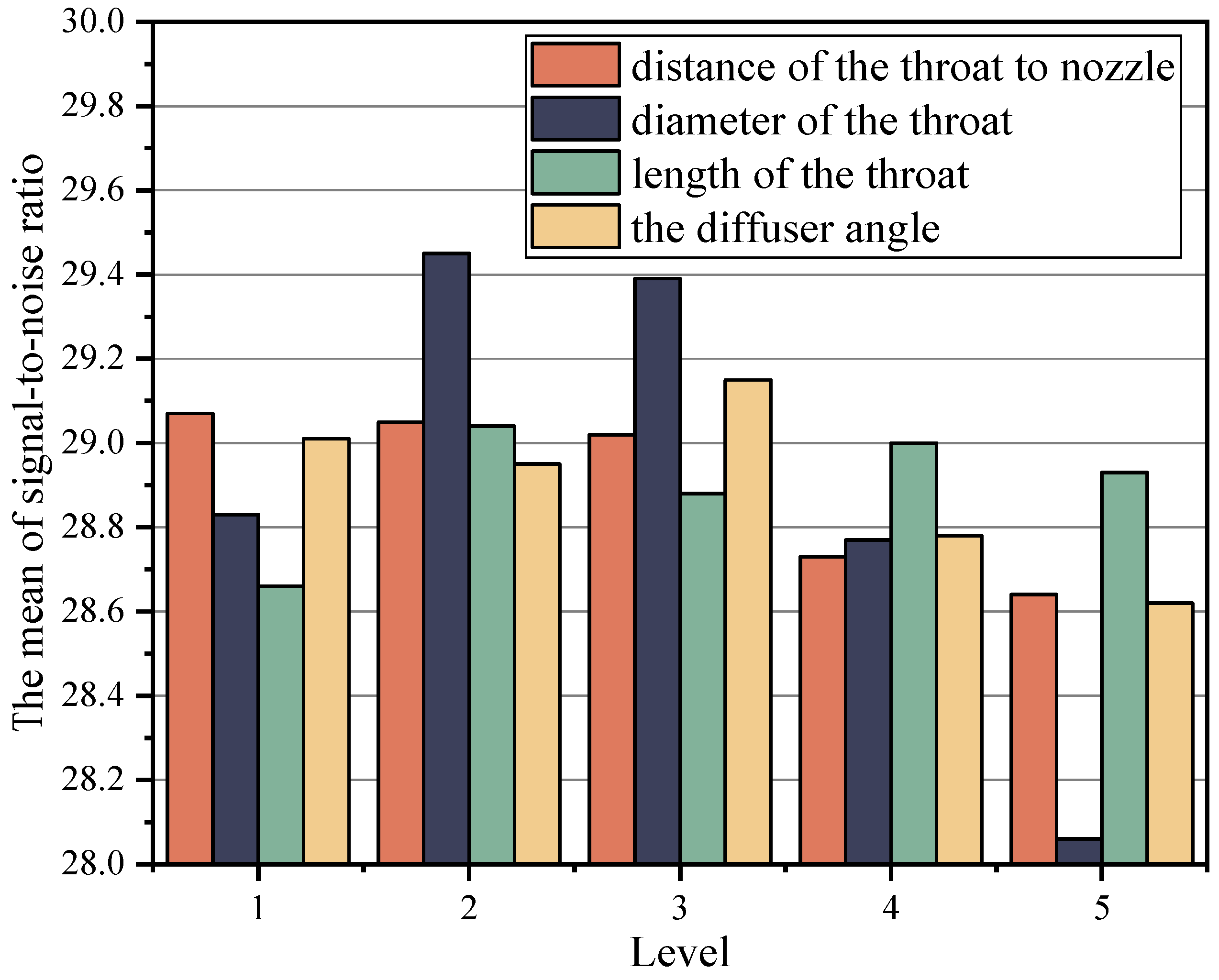
| 1 | 29.07 | 28.83 | 28.66 | 29.01 |
| 2 | 29.05 | 29.45 | 29.04 | 28.95 |
| 3 | 29.02 | 29.39 | 28.88 | 29.15 |
| 4 | 28.73 | 28.77 | 29.00 | 28.78 |
| 5 | 28.64 | 28.06 | 28.93 | 28.62 |
| Delta | 0.43 | 1.39 | 0.38 | 0.53 |
| Rank | 3 | 1 | 4 | 2 |
| Level | Distance from the Throat to the Nozzle | Diameter of the Throat | Length of the Throat | The Diffuser Angle |
|---|---|---|---|---|
| (mm) | (mm) | (mm) | (°) | |
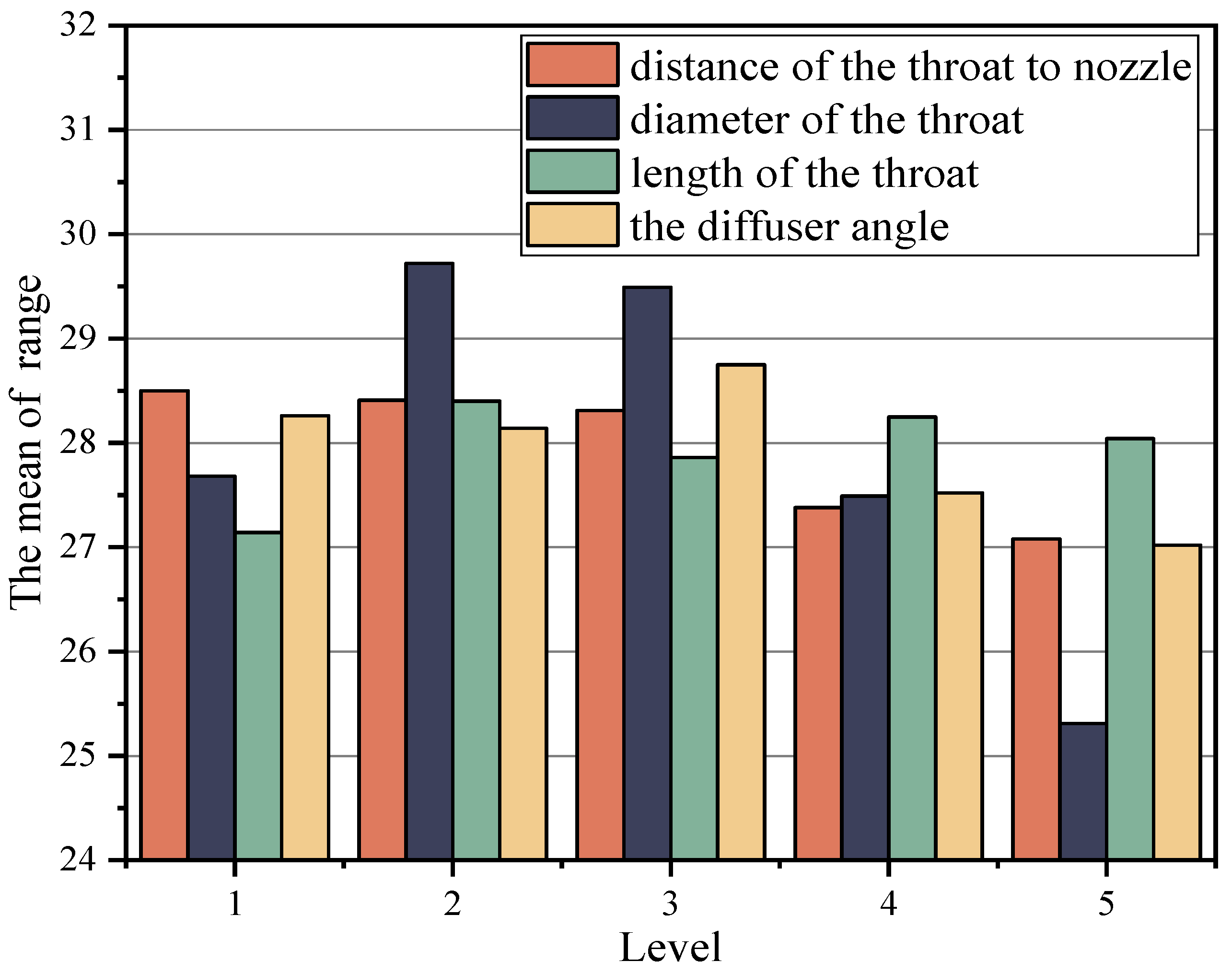
| 1 | 28.50 | 27.68 | 27.14 | 28.26 |
| 2 | 28.41 | 29.72 | 28.40 | 28.14 |
| 3 | 28.31 | 29.49 | 27.86 | 28.75 |
| 4 | 27.38 | 27.49 | 28.25 | 27.52 |
| 5 | 27.08 | 25.31 | 28.04 | 27.02 |
| Delta | 1.44 | 4.41 | 1.26 | 1.72 |
| Rank | 3 | 1 | 4 | 2 |
| Control Factors | Quadratic Sum | Degree of Freedom | Variance | Values of F | Contribution Degree |
|---|---|---|---|---|---|
| Distance from the throat to nozzle | 0.766 | 4 | 0.192 | 1.721 | 9.12% |
| Diameter of the throat | 6.378 | 4 | 1.595 | 14.293 | 75.93% |
| Length of the throat | 0.446 | 4 | 0.112 | 1.004 | 5.31% |
| The diffuser angle | 0.810 | 4 | 0.203 | 1.819 | 9.64% |
| The New Jet Pump | Distance from the Throat to the Nozzle | Diameter of the Throat | Length of the Throat | The Diffuser Angle | Flow Ratio | Pump Efficiency |
|---|---|---|---|---|---|---|
| (mm) | (mm) | (mm) | (°) | (%) | ||
| Before optimization | 10.44 | 6.65 | 40 | 8.0 | 0.3156 | 21.81 |
| After optimization | 2.62 | 6.80 | 46 | 7.5 | 0.3156 | 31.26 |
Disclaimer/Publisher’s Note: The statements, opinions and data contained in all publications are solely those of the individual author(s) and contributor(s) and not of MDPI and/or the editor(s). MDPI and/or the editor(s) disclaim responsibility for any injury to people or property resulting from any ideas, methods, instructions or products referred to in the content. |
© 2023 by the authors. Licensee MDPI, Basel, Switzerland. This article is an open access article distributed under the terms and conditions of the Creative Commons Attribution (CC BY) license (https://creativecommons.org/licenses/by/4.0/).
Share and Cite
Wang, Z.; Lei, Y.; Wu, Z.; Wu, J.; Zhang, M.; Liao, R. Structure Size Optimization and Internal Flow Field Analysis of a New Jet Pump Based on the Taguchi Method and Numerical Simulation. Processes 2023, 11, 341. https://doi.org/10.3390/pr11020341
Wang Z, Lei Y, Wu Z, Wu J, Zhang M, Liao R. Structure Size Optimization and Internal Flow Field Analysis of a New Jet Pump Based on the Taguchi Method and Numerical Simulation. Processes. 2023; 11(2):341. https://doi.org/10.3390/pr11020341
Chicago/Turabian StyleWang, Zhiliang, Yu Lei, Zhenhua Wu, Jian Wu, Manlai Zhang, and Ruiquan Liao. 2023. "Structure Size Optimization and Internal Flow Field Analysis of a New Jet Pump Based on the Taguchi Method and Numerical Simulation" Processes 11, no. 2: 341. https://doi.org/10.3390/pr11020341