

Designing Dispatching Rules via Novel Genetic Programming with Feature Selection in Dynamic Job-Shop Scheduling
School of Mechanical Engineering, Xinjiang University, Urumqi 830047, China
*
Author to whom correspondence should be addressed.
Processes 2023, 11(1), 65; https://doi.org/10.3390/pr11010065
Submission received: 24 November 2022
/
Revised: 23 December 2022
/
Accepted: 25 December 2022
/
Published: 27 December 2022
(This article belongs to the Special Issue Computer-Aided Manufacturing Technologies in Mechanical Field)
Abstract
:Genetic Programming (GP) has been widely employed to create dispatching rules intelligently for production scheduling. The success of GP depends on a suitable terminal set of selected features. Specifically, techniques that consider feature selection in GP to enhance rule understandability for dynamic job shop scheduling (DJSS) have been successful. However, existing feature selection algorithms in GP focus more emphasis on obtaining more compact rules with fewer features than on improving effectiveness. This paper is an attempt at combining a novel GP method, GP via dynamic diversity management, with feature selection to design effective and interpretable dispatching rules for DJSS. The idea of the novel GP method is to achieve a progressive transition from exploration to exploitation by relating the level of population diversity to the stopping criteria and elapsed duration. We hypothesize that diverse and promising individuals obtained from the novel GP method can guide the feature selection to design competitive rules. The proposed approach is compared with three GP-based algorithms and 20 benchmark rules in the different job shop conditions and scheduling objectives. Experiments show that the proposed approach greatly outperforms the compared methods in generating more interpretable and effective rules for the three objective functions. Overall, the average improvement over the best-evolved rules by the other three GP-based algorithms is 13.28%, 12.57%, and 15.62% in the mean tardiness (MT), mean flow time (MFT), and mean weighted tardiness (MWT) objective, respectively.
1. Introduction
Production scheduling aims to assign available production resources to several different demands within a reasonable running time in order to optimize one or more target values [1,2]. The Job shop scheduling (JSS) problem has attracted much interest from academics and industry experts due to its extensive applications and inherent difficulties in the manufacturing area [3,4]. A set of jobs and machines are given on the job shop floor, and each job contains several operations that need to be executed by an appropriate machine. Then, the goal of JSS is to construct a scheduling procedure that processes the operation with machines under a predefined sequence to optimize some defined objectives, such as minimizing the makespan, flow time, and tardiness [5].
In general, job shop conditions can be divided into static and dynamic. Jobs are ready for processing at time zero in static conditions, and their operational information, such as arrival time, number of operations, and due date, is always available. Unlike the static environment, dynamic job shop scheduling (DJSS) deals with situations where job arrivals are usually unknown in advance. The processing attributes can only be obtained gradually over time. Therefore, traditional search-based techniques that are capable of obtaining high-quality solutions are not applicable because they search a solution space that is not only computationally expensive but also too slow to react adequately to unanticipated disruptions such as the arrival of new jobs, a change in the due date, or the malfunctioning of machines. Thus, scheduling heuristics that deliver acceptable but not necessarily optimal solutions in a short computational time have been employed to solve DJSS. Due to its adaptability, low time complexity, and rapid response to varying conditions, the dispatching rule, which is a particularly simple type of scheduling heuristic, is now widely used [6]. In each decision situation, the dispatching rule decides the job with the highest priority value to be scheduled next when a machine is free. However, dispatching rules are challenging to design manually due to these reasons. It is hard to determine the relative factors from the various job shop characteristics and to understand their influence on rule performance. In addition, selecting and testing the best dispatching rules through complex simulation runs in job shop scenarios is very time-consuming.
In recent years, researchers have devoted more attention to automated heuristic design, which uses AI and machine learning to address complicated computational issues known as “Hyper-heuristics.” [7]. This approach is motivated by a desire to shorten the time required for experts to design effective heuristics for various circumstances and to get important insights by investigating a broad variety of unexplored heuristics [8]. Genetic Programming (GP) is a well-known hyper-heuristics approach for creating efficient scheduling heuristics for a variety of industrial applications [9,10]. Due to the powerful search engine, GP can automatically determine the structure and parameters of the program compared to other artificial intelligence methods. The three factors: maximal depth of the tree, function set, and terminal set, are the factors that determine the GP search area. Therefore, decreasing the number of terminals is one of the ways to reduce the scope of GP search and enhance the search capability. In DJSS, a wide range of features can be included in the terminal sets, such as system-related, job-related, and machine-related features [11,12]. Previous studies often consider all the potential attributes to construct GP trees. Not all the attributes in the terminal section are helpful, and some might be unrelated or redundant for producing superior dispatching rules in the specific job shop settings. For example, the due date of the job is considered to be a useless feature for optimizing the mean flow time. Similarly, the weight of the job plays an important role if the objective is mean-weighted tardiness rather than mean flow time. Therefore, selecting important terminal sets for different scenarios is challenging without losing promising areas in the search space.
Feature selection in machine learning provides a good idea for solving this challenging task. It has been proven to be an effective way when dealing with classification [13,14], clustering [15], and regression tasks [16]. Although GP can identify relevant features and use them to evolve the best GP trees simultaneously in the adaptive evolutionary process, there are still some irrelevant or redundant features. More in-depth research is needed in this area.
As far as we know, there is little research on feature selection in DJSS. The feature selection approach that calculates the terminal frequency in the best-evolved rules was designed to improve the evolutionary ability of GP [17]. A novel feature selection method instead of frequency was first introduced to identify the crucial features for different job shop scheduling situations [18]. To improve the efficiency of feature selection, an efficient feature selection algorithm with niching and surrogate techniques was proposed to produce superior dispatching rules in dynamic job-shop scenarios [19]. The construction of dispatching rules for the flexible DJSS issue was then proposed using a novel two-stage genetic programming-based hyper-heuristic (GPHH) framework with feature selection and individual adaptive strategy [20]. However, the existing feature selection approaches in GP evolution for DJSS have revealed some challenges and gaps in the current approaches, as described below:
- (1)
- Most feature selection methods assess the effect of each terminal by the frequency with which it occurs in the best-evolved rules. The main shortcoming of this technique is that the results may be biased towards irrelevant features because of the occurrence of redundant features.
- (2)
- Obtaining a diverse set of excellent individuals is a challenging task and is considered a key factor in achieving high accuracy in feature selection. Although the niching-based GP feature selection method has been proven to be an effective algorithm, it is still difficult and complex to determine the parameter of the niche.
- (3)
- The proposed feature selection approaches for DJSS are usually based on the mode of offline selection mechanisms or a checkpoint to obtain relative terminal sets. This offline approach not only requires a significant expenditure of time and code effort but may also waste some of the excellent individual structures that have been generated during the feature selection process.
- (4)
- The enhancement of the solution quality of dispatching rules in different job shop scenarios is not taken into account by current techniques, which primarily concentrate on rule interpretability via the feature selection process.
Therefore, this paper aims to address the literature limitations by proposing an integration approach that combines a novel GP method with a feature selection mechanism to design interpretable and high-quality dispatching rules for DJSS. The main contributions of this work can be summarized as follows:
- (1)
- Develop a three-stage GP framework to utilize the information of both the selected features and the promising diverse individuals in the feature selection process.
- (2)
- Propose a novel GP method, GP via dynamic diversity management, with a feature selection mechanism to acquire compact, interpretable, and high-quality rules for DJSS automatically. In this strategy, the level of population diversity is related to the stopping criterion and the time elapsed to gradually adjust the search space of the algorithm from exploration to exploitation.
- (3)
- Verify the effectiveness of the proposed approach compared to the three GP-based algorithms and 20 benchmark rules from the existing literature under mean tardiness, mean weighted tardiness, and mean flowtime objectives, respectively.
The rest of the paper is organized as follows: The problem description and literature on the automated design of dispatching rules, genetic programming-based hyper heuristic, and genetic programming with feature selection are reviewed in Section 2. The suggested technique is detailed in Section 3, while Section 4 provides the experimental design. Section 5 covers the experimental results and discussions, and further analysis is provided in Section 6. Finally, conclusions and future recommendations are given in Section 7.
2. Background
2.1. Problem Definitions for DJSS
The Dynamic Job Shop Scheduling (DJSS) problem is a typical optimization problem that can be described as follows. The job shop floor has a number of machines. An arriving job has a sequence of operations .The th operation of job , denoted as . Each operation can only be processed by its eligible machine , and its processing time is denoted as (abbreviated as ). The time when the job arrives on the shop floor is the operation ready time of the first operation of job (labeled as ) and is referred to as the release time of the job [21]. A job also has a due date . This paper focuses on DJSS problems with dynamic job arrival, which means that the properties of a job can only be known when it arrives.
2.2. Related Work
Automated design of dispatching rules. Job shop scheduling problem (JSSP) as an NP-complete combinatorial optimization problem [3]. Due to this, accurate optimization techniques are difficult for solving large-scale production issues [22]. Therefore, approximate optimization methods such as genetic algorithm [23], simulated annealing [24], and ant colony algorithm [25] have been developed to find quasi-optimal solutions for static JSSP in an acceptable amount of computing time. Under dynamic conditions, traditional scheduling methods are impractical due to the limited information horizon in DJSS problems, which need precise job shop information in advance. Therefore, dispatching rules is considered an effective heuristic search method for real-time events for dealing with DJSS problems. Specifically, the dispatching rule assigns a score to each waiting job according to its priority function when a machine is available. Then, the job with the highest priority among the waiting ones is then selected to be processed next. Numerous research has been conducted to manually establish suitable dispatching rules for a variety of workshop situations and goals. More details are available in several articles [26].
The manual design of dispatching rules begins with creating a collection of job shop qualities, then attempting to achieve the optimal mathematical combination of these terminals. All candidate rules are then hard-coded and assessed using a discrete event simulation (DES) model. This cycle is conducted several times to determine the optimal rule for optimizing a performance metric under specific job shop conditions. Since man-made dispatching rules cannot achieve satisfactory performance, many researchers aim to develop a hyper-heuristic approach that can automatically discover adaptive rules for the JSS problems. Hyper-heuristics combine the components utilized in current heuristics by different operators to build new heuristics, which are then trained on training problem cases and developed to become more successful. Regarding the automated construction of scheduling rules, it has been shown that GP is a promising hyper-heuristic method that outperforms conventional machine learning techniques [27].
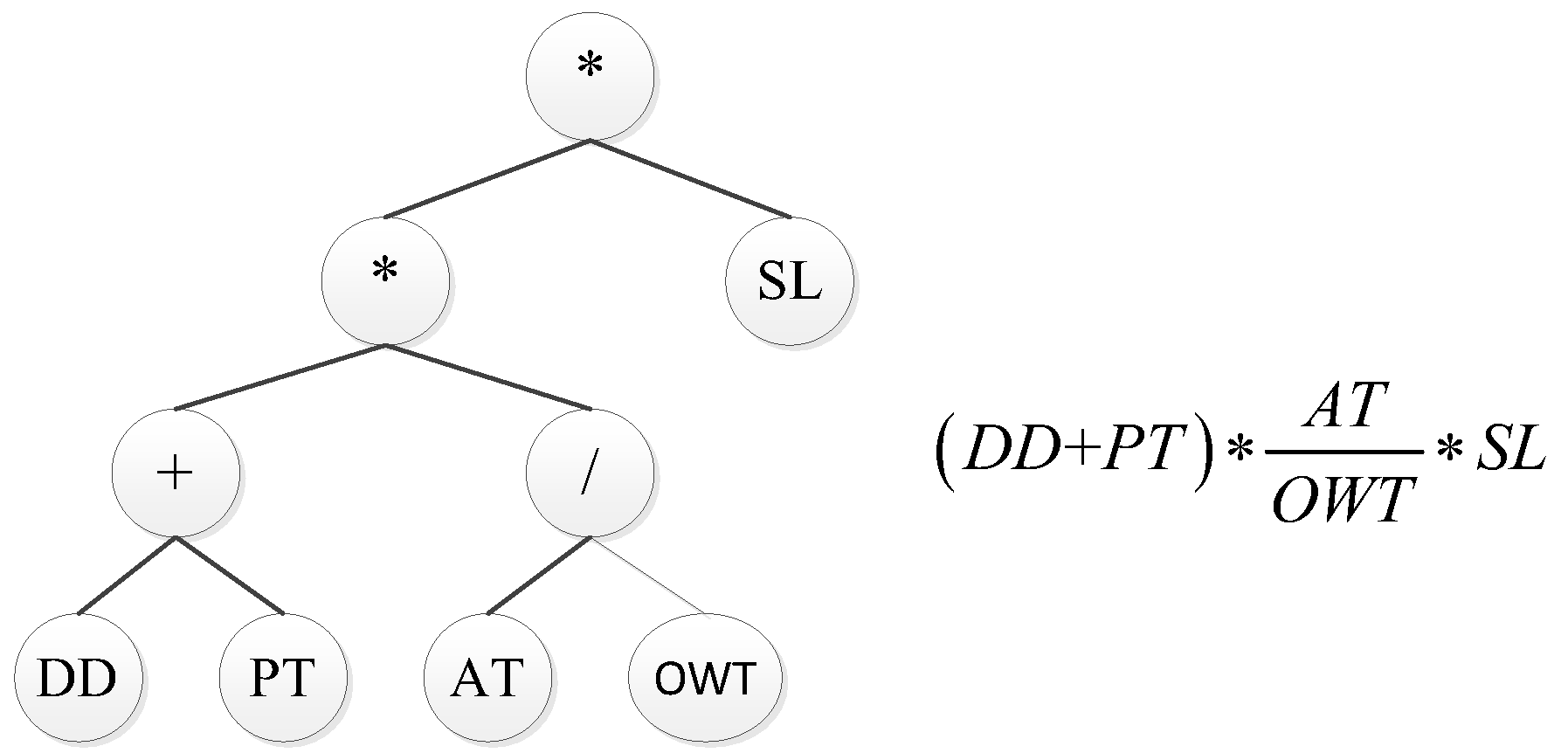
Genetic programming-based hyper-heuristic. As a hyper-heuristic method, GP can automatically design new dispatching rules based on structure and parameters without rich domain knowledge. Individuals in GP may be represented in several ways [28], with the tree-based representation being the most common. The intuitive nature of the GP’s individual representation approach allows it to build trees of various formats and lengths, making it suited for use as a hyper-heuristic in automatically producing dispatching rules. Figure 1 gives an example of a parse tree and the corresponding dispatching rule. The tree is usually interpreted from left to right in depth-first order.
The GPHH technique examines the space of heuristics via the GP to uncover the heuristics that may be utilized to successfully address the production scheduling difficulties. Burke et al. [7] presented a categorization of hyper-heuristic techniques according to their search process, which includes choosing and creating hyper-heuristics. A quick overview of hyper-heuristic applications for a variety of scheduling and combinatorial optimization issues was also provided. According to the authors, GP is well suited for adapting dispatching rules in dynamic situations, even if it is seldom employed to directly handle production scheduling problems. The article by Branke et al. [1] included a comprehensive analysis of the design decisions and important concerns that arose throughout the course of the development process. In the survey, significant design considerations such as feature selection, rule representation, and fitness function analysis are discussed. In the same context, Nguyen et al. [29] present an overview of the automated design of dispatching rules in the area of production scheduling using genetic programming. They provided a detailed discussion of the key components and practical issues that should be considered before developing a GP system for generating production scheduling heuristics. This article also showed that the number of works on the subject of automated design of scheduling heuristics had increased significantly since 2010. Branke et al. [28] studied the automatic construction of dispatching rules in DJSS by comparing GP in a tree structure, neural network, and linear representation. The GP tree form offered the highest quality answer, followed by the neural network representation, while the linear representation yielded the lowest outcomes. One major factor is that the GP method concurrently investigates a heuristic’s structure and associated parameters without supposing any specific distribution or domain expertise.
In addition to the above research, the GPHH approach has been utilized to generate scheduling heuristics for production scheduling problems with diverse characteristics, such as the DJSP with dynamic job arrivals and machine breakdowns [30,31] and the dual-constrained flow shop scheduling with machines and operators [32]. Furthermore, several research projects aimed at increasing the performance of the GPHH technique using diverse strategies. By using ensemble learning for the ensemble GPHH technique through different combination strategies for the DJSP, Park et al. [33] increased the robustness of the GPHH approach. Zhou et al. [34] proposed a surrogate-assisted cooperative coevolution GP technique for the dynamic flexible JSP, which increased the computational efficiency and the offline learning process of the hyper-heuristic without compromising its performance.
Genetic programming with feature selection. Regardless of the chosen representation, the selection of appropriate job and shop characteristics that constitute the evolvable components of priority functions is a crucial design issue. In DJSS, the terminal set may consist of different shop attributes for constructing dispatching rules. The list of attributes could be anything from common attributes (e.g., the processing time of the operation) to multiple attributes (e.g., the remaining processing time of the job), but not all of them are equally relevant in a specific job shop case. Removing the irrelevant and redundant attributes in evolving dispatching rules may bring the following benefits. First, it will improve GP’s searchability by reducing search space. Scend, GP tends to derive effective, compact, and meaningful dispatching rules without irrelevant or redundant attributes. Third, it can reduce the computational time of GP with shorted rules. In order to create compact and interpretable dispatching rules, it is important to select the vital few attributes for the different scenarios. Although GP can detect the hidden relationships between a subset of features, it is not very effective and accurate. Previous research has shown that the best individuals still have some irrelevant and redundant features. In other words, GP’s ability is limited. Several academics have advocated attribute selection or simplification as a means to decrease the number of terminals accessible for the evolution of dispatching rules.
Friedlander et al. [17] suggested a feature selection approach based on frequency analysis, that is, the number of times a certain terminal appears in rules (genotypic analysis). This approach has its own limitation: some features are incorrectly estimated based on their frequency in the redundant priority function. Therefore, Mei et al. [18] proposed an offline feature selection approach in GP, which measures the importance of features based on their contribution to the priority function. Although this method can select the important features more accurately, it requires expensive computational time to obtain a set of good individuals with diversity. In a follow-up study, Mei et al. [19] designed an offline feature selection algorithm with niching and surrogate techniques to produce superior dispatching rules in DJSS. Specifically, a niching-based GP algorithm was applied to initially obtain a set of good individuals with diversity. Then, the feature’s contribution to the performance of good rules was estimated using a weighted voting mechanism. Finally, the selected terminal set was applied to evolve the best rules in future GP runs. The limitation of this work is that the program size of the evolved rules is still large, even though the approach is sufficient to identify a compact set of features. Nguyen et al. [35] added an attribute vector to the tree representation of each rule in an effort to improve the interpretability of the rules by choosing relevant characteristics. The most significant restriction is that it disregards scenarios in which a certain property may not be included in the priority function. Based on Nguyen’s research [35], Shady et al. [36] proposed a new representation of the GP rules by modifying the attribute vector that abstracts the importance of each terminal during the evolution process. Later, Shady et al. [37] extended this attribute vector into the liner representation of gene expression programming (GEP) to evolve effective rules in simple structures with an affordable computational budget. Moreover, Panda et al. [38] suggested a novel GP with simplification for DJSS and examined its effectiveness in developing effective and simple/small rules. In addition to adopting the general algebraic simplification operators, additional problem-specific numerical and behavioral simplification operators were designed for DJSS. Huang et al. [39] developed scheduling strategies for multitasking issues utilizing the building block reuse of liner genetic programming. Fan et al. [40] employed the GPHH approach to solving DJSS with extended technical precedence restrictions. To improve the performance of GP-evolved rules, they proposed problem-specific GP attribute selection by incorporating store state information that is important for scheduling. Recently, Zhang et al. [20] proposed a novel two-stage GPHH framework with feature selection and individual adaptive strategies for the flexible DJSS problem. Using a predetermined checkpoint, this approach separates the whole GP procedure into two phases. A niching-based method combined with a surrogate module to achieve selected terminals in the first phase. While the new terminal replaces the original one, it is used for individual evolution after checkpoint generation in the second stage. Although this feature selection framework was adapted online and obtained compact rules, it neglected to consider the improvement of rule performance.
There is, as already suggested, a growing body of research literature on the design of scheduling rules with attribute selection or simplification, but there are still some gaps in rule interpretability and the impact of improved strategies on rule performance that deserve attention. The focus of the recent literature is obtaining more compact rules with fewer features rather than improving the performance of evolved rules. Few studies have considered both feature selection mechanisms and rule quality improvement. Therefore, this work aims at designing interpretable and high-quality rules simultaneously for the DJSS problem.
3. Proposed Methods
3.1. Framework of the Proposed Approach
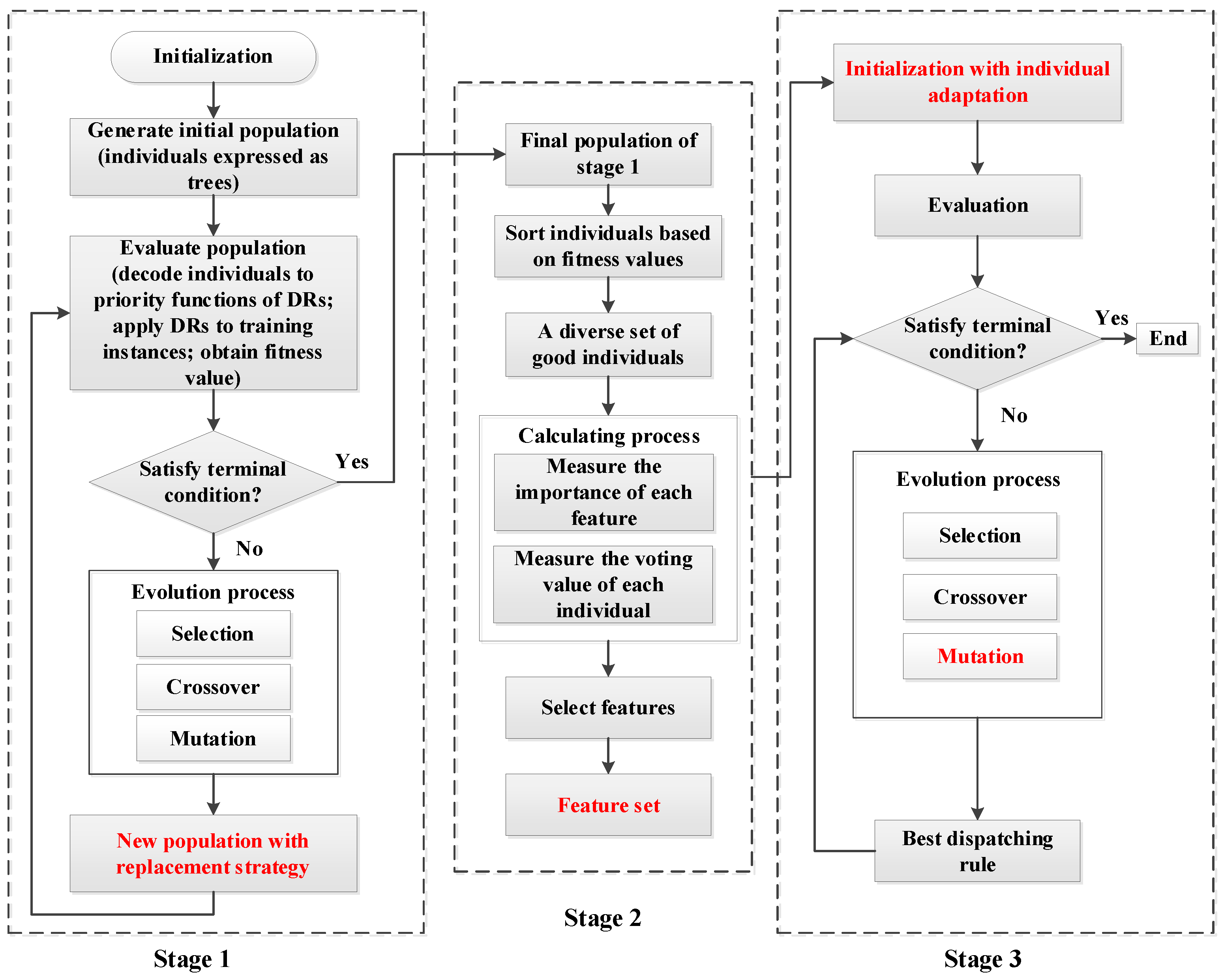
The existing literature on feature selection methods for DJSS generally employs an offline selection mechanism. The overall process is usually divided into two parts, in which feature selection is taken as a preprocessing step to obtain the feature set first. Then the selected features are used in another independent GP run to solve the DJSS problem. The whole process is completed independently and separately, which is time-consuming and impractical. In order to evolve high-quality rules with compact structures effectively, this paper proposes a novel GP algorithm with online feature selection based on the idea in Zhang’s research [20]. As illustrated in Figure 2, the framework of the proposed approach comprises of three steps. In the first stage, the GP proceeds with a diversity management strategy that considers the stopping criterion and elapsed period to obtain a diverse set of superior individuals for feature selection. An essential feature of this diversity management strategy is the dynamic penalization scheme that considers similarity measures between individuals in the replacement phase. This way, a diverse set of best dispatching rules can be derived, which is a key factor in achieving high accuracy in feature selection [19]. In the second stage, the feature selection mechanism is carried out to obtain feature subsets based on the final population obtained in the first phase for the different scenarios. Based on the final population with individual adaptation and selected feature subsets getting from previous steps, stage three is used to evolve more compact and high-quality rules. In the third stage, the standard GP algorithm is used, except for the initialization and mutation process. The initialization process takes the final population of stage 1 as the initial population. The standard subtree mutation is applied by generating random trees using only the selected features.
3.2. A Novel GP Method
Diversity management in the population is crucial to the success of evolutionary algorithms. In the case of GP, several methods and strategies have been developed to measure diversity or maintain the level of population diversity [41,42]. Recently, Ricardo et al. proposed a design concept for GP that relates the level of population diversity to the stopping criterion and the time elapsed to enhance the performance of GP in symbolic regression problems [43]. The most important feature of this design principle is the inclusion of a dynamic penalization scheme in the replacement phase, which aims to avoid the existence of similar individuals. Compared with other diversity management schemes, it has been demonstrated to be competitive in solving combinatorial optimization problems. Inspired by their research, this paper applies this idea but explores it for the DJSS problem in production scheduling.
- (1)
- The replacement strategy: The pseudocode of the proposed replacement strategy in GP is described in Algorithm 1. The algorithm aims to select the number of desired survivors to create a new population for the next generation. Initially, the current population and offspring are added to create a set of candidates . Since the fitness in this article is to be reduced, the smallest candidate is chosen and removed from the present candidates and utilized to create a new population. A threshold value is then computed for penalizing the candidates in subsequent steps (line 4). After the previous initial steps, the survivors are chosen from the candidate set to create the new population through iterations (see lines 5–15). The algorithm categorizes the candidates into the penalized set () and the non-penalized set () at each iteration (line 6). To be specific, any candidate with a distance to the nearest survivor below the threshold , is classified as a penalty candidate or else as a non-penalized candidate. If there are non-penalized candidates, a multi-objective method that considers fitness and simplicity is used to choose randomly dominated candidates, while penalized candidates are disregarded. If there are non-penalized candidates, a multi-objective selection procedure that takes into account fitness and simplicity is applied to select randomly dominated candidates, with penalized individuals being overlooked (lines 7–9). Otherwise, if all candidates are penalized, the algorithm will choose the farthest (line 11). It may imply that the population diversity is too limited under this condition; thus, it seems more promising to select the individual with the farthest distance. Lastly, the selected candidate is removed from the candidates set and incorporated into the new population.
Input: A current population , offspring , number of survivors , elapsed iterations , termination criterion , initial distance threshold Output: New Population 1 ; 2 ; 3 ; 4 ; 5 while do 6 categorize-individuals ; 7 if then
8 non-dominated-set9 random-sampling 10 else 11 farthest 12 end
13
14
15 end
16 return
- (2)
- Phenotypic Characterization of Dispatching Rules: The minimum required distance function used in Algorithm 1 to establish the threshold value, which is then utilized to distinguish between individuals who are penalized and those who are not. The threshold is a dynamic value that decreases linearly during the evolution process. This indicates that more closely related individuals are accepted as the iteration goes on, gradually moving the focus away from exploration and toward exploitation. In this way, the dynamic threshold automatically focuses the search toward the most promising areas in the final stage of the optimization.
In this paper, the threshold is set as follows:
where is the initial distance value, is the average of the closest distance between individuals in a population , is the elapsed iterations, is the stopping criterion.
In the above threshold function, a distance measure between two rules and is needed. Different from traditional tree distance measures like distance, it is possible that two rules with different genotype structures will make the same behavior decisions in GP tree. So, the distance metric should reflect the difference in phenotypic behavior, not the difference in genotype structure. Therefore, this paper employs phenotypic characterization of dispatching rules based on a decision vector [44], which is a record of all decisions made by a rule under decision situations . Specifically, the reference dispatching rule is first used to rank all candidate jobs in to obtain the ranking vector . The rule to be characterized is also applied to rank the jobs to obtain the ranking vector . Then, the index of the jobs with the highest priority assigned by the reference rule is identified. Finally, the rank of the th job in the ranking vector is set to the th element of the characteristic vector. In Algorithm 2, this phenotypic characterization of dispatching rules is described in pseudocode.
| Algorithm 2. Compute the phenotypic characterizationof dispatching rule. |
| Input: the dispatching rule to be characterized, the reference rule , set of decision situations . |
| Output: decision vector . |
| 1 for do; |
| 2 ; for each decision situation |
| 3 ; determine ranks, highest priority gets rank 1 |
| 4 ; |
| 5 |
| 6 |
| 7 end for 8 return |
3.3. Feature Selection
In this paper, the feature selection idea is taken from Mei’s research [19], which considers the importance of features related to both individual fitness and its contribution to individuals. Therefore, given a set of good and diverse individuals , features can be selected by a Feature Selection function . Algorithm 3 describes the pseudo-code of the feature selection approach. First, a certain number of top individuals with better fitness values are selected from the final population at stage 1, and then taken as diverse and good individuals . Second, the contribution of each feature to each individual is measured by (4), where denotes the fitness value of the rule that fixed the feature with the constant of 1. For example, . A positive value of indicates that the rule performance becomes worse after removing the feature . So, the measured feature can be given voting weight from the rule .
Since the objective functions included in this article are to be minimized, the smaller the fitness of dispatching rules, the greater their voting weights. Then, the “voting weight” of a dispatching rule should be a monotonically decreasing function of its fitness. The calculation is given by (5)–(8). Finally, if the weight voting for a feature is greater than the weight against it, the feature is selected (from lines 10 to 13).
| Algorithm 3. Feature Selection process. |
| Input: A set of good and diverse individuals . |
| Output: The selected feature set F. |
| ; |
| do |
| do |
| by Equation (4); |
| by Equations (5)–(7) |
| then |
| 7 |
| 8 end 9 end |
| 10 if then 11 ; 12 end 13 end 14 return F |
3.4. Individual Adaptation Strategy
In the third stage, the promising individuals obtained from the novel GP algorithm and the selected features are utilized to evolve interpretable and high-quality rules. However, there are still unselected features in the final population. To address this problem, two representative individual adaptation strategies have been proposed in previous studies [20]. Setting the unselected feature in the dispatching rule to a constant number one is a common strategy. Another works by assuring that phenotypically similar individuals evolving only with selected features replace the promising ones in the final population at stage one. The experimental results obtained in their research show that both strategies can effectively inherit information from the final population of individuals. It also demonstrated that the first strategy has a more promising inheritance ability compared to the second. Therefore, in order to reduce the computing costs of generating behavioral similar individuals, the first strategy is adopted to eliminate the unselected features while retaining the individual structure as much as possible. The standard GP algorithm is used in the third stage, except for the initialization and mutation process. In the initialization process, the first part of the initial population contains the promising individuals from the novel GP algorithm, while the remaining part stores the random individuals evolved by the selected features. The standard subtree mutation is applied by generating random trees using only the selected features.
4. Experimental Design
To investigate the effectiveness and interpretability of the proposed approach in a wide range of scenarios, a set of experiments has been designed.
4.1. Discrete Event Simulation Model
To evaluate various GP-HH methods for DJSS, discrete event-based simulations have been designed in previous literature [35,45]. In our experimental settings, there are ten machines; jobs are released, and they arrive at the shop stochastically. Job parameters are randomly generated, such as the route of the job, the processing time, the number of operations, etc. Job arrival follows a Poisson process with rate which is based on a predetermined utilization . The number of operations per job is randomly sampled from 2 to 10, and the mean processing time of each operation is sampled between 25 and 100. Job due dates are assigned using the total work content method with different tightness factor values. In terms of the weights of the jobs, the 4:2:1 rule recommended by Shady’s research is adopted [36].
In the experiment, the job shop starts running from an empty state; a warm-up time period is needed to achieve a reliable state. The statistics are only recorded for the 501st through 2500th jobs to assess the performance of dispatching rules. To evaluate the effectiveness of the designed rules, it is necessary to define a wide range of scenarios reflecting different types of problem instances. A simulation scenario is represented by a tuple 〈〉 whose parameters are described in Table 1. Past research has shown that the tightness factor and machine utilization are the main factors to define the load conditions, which play a major part in rules’ performance. This article takes into account both light-load and heavy-load situations in order to assess the quality of the created rules. To do this, two or three values are set for α and μ in the job-shop simulation, ranging from 2 to 7 and 80% to 99%, respectively. Simulator runs a single replication for each scenario during the training phase. For testing the generated rules, 20 simulation replications are executed for each test configuration.
The objective functions investigated in this paper are Mean Tardiness (MT), Mean Weighted Tardiness (MWT), and Mean Flow Time (MFT), respectively. MT and MWT are given in Equations (9) and (10), where is the completion time of job , and is the weight of the job . denotes the set of delayed jobs, while represents the collection of completed jobs. In addition, Equation (11) is used to estimate the MFT objective, where means the flowtime of job .
Moreover, when evaluating the overall performance of each dispatching rules , the fitness function is calculated by Equation (12), where is the value of scheduling objective, which is calculated by applying the rule to a training instance , denotes the target value, obtained by the reference rule in the same training instance. Due to the impressive results for minimizing the MT, MWT, MFT objectives, the Covert, WATC, PT+WINQ rules are adopted as reference rules, respectively [5,19].
4.2. Algorithm Parameters
Table 2 includes the list of terminal and function sets. The terminal set used for the experiment contains the common features used in the existing literature about GP-HH approaches [19,20,36]. These features range from job-related features (e.g., the number of operations remaining for a job NOR) to machine-related terminals (e.g., waiting time of a machine) and the current state of the shop (e.g., current time NOW). Four traditional mathematical operators “,” are included in the function set. The operator “” works as a protected division, returning a value of 1 in the case of the dominator is zero. Also, the “max” and “min” functions are used.
Details of other parameter settings of the algorithm are listed in Table 3.
4.3. Comparison Design
In order to validate the achievements of the proposed approach (NGP-FS), three algorithms are considered for comparison. The standard genetic programming algorithm (SGP) without feature selection is adopted as the baseline approach. The SGP with feature selection approach, designated as SGP-FS, is compared to investigate the impact of the online feature selection mechanism on the standard GP algorithm. Additionally, the novel genetic algorithm (NGA) is compared to determine if dynamic diversity management in GP without feature selection enhances the algorithm’s ability to develop concise and high-quality dispatching rules. All methods are evaluated and compared according to the solution quality and interpretability of the rules. In addition, the rule performance is also compared to the representative benchmark rules, as given in Table 4.
5. Results and Discussion
The experimental findings of the evolved rules for three objective functions are presented in this section. As mentioned earlier, the proposed NGP-FS approach is compared to SGP, SGP-FS, and NGP to verify its effectiveness. The three key performance metrics, including test performance, mean rule length (number of nodes), and computational time, are applied to compare the four GP-based methods. For these three metrics, the smaller the metrics, the better the evolved rules’ performance. For statistical significance testing, the Wilcoxon rank sum test is used, with a significance level of 0.05.
5.1. Training Performance
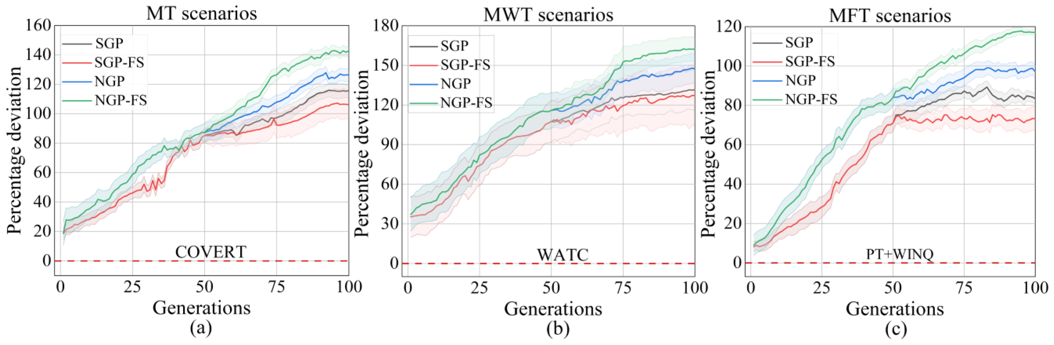
Table 5 shows the statistical analysis of the proposed algorithm NGP-FS compared to the three algorithms in the three objective functions. The marks “+”, “−”, and “=” inside the findings indicate that the associated result is considerably superior to, inferior to, or equal to its counterparts, respectively. The test performance of the evolved rule is defined as the percentage deviation from the reference rule, i.e., , where is estimated by Equation (12). The percentage deviation for the MT, MWT, and MFT targets is shown in Figure 3a–c, respectively.
Concerning the performance of the designed rules, the NGP-FS algorithm outperforms all other algorithms for the three analyzed goals. It is also noted that the SGP-FS algorithm performs poorly in all objectives. It seems counter-intuitive because feature selection is considered an effective way to reduce irrelevant features in the GP algorithm to enhance the quality of the solution. However, this might indicate that the quality of the final population from stage 1 affects the accuracy of feature selection, even though the same adaptation strategy and mutation process are used for SGP-FS and NGP-FS in stage three.
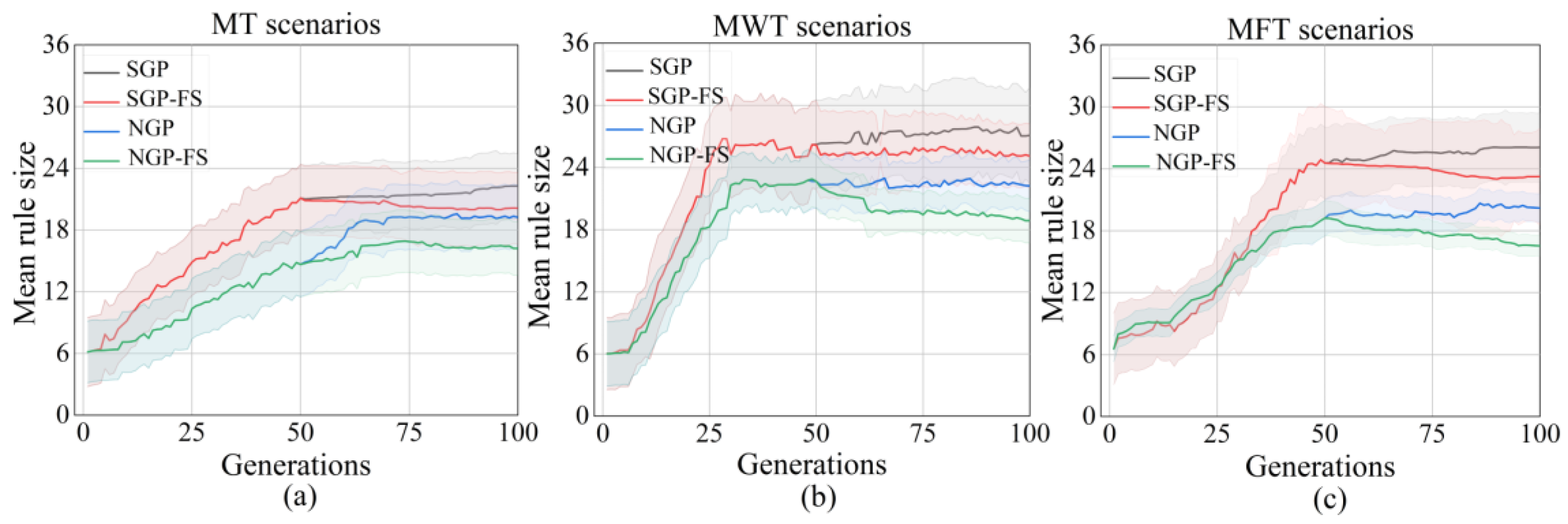
Evolving compact and easily interpretable dispatching rules is important in scheduling tasks. An important factor that concerns interpretability is the rule size, which is usually defined as the number of nodes included in a rule. The concise dispatching rules provide an advantage in reduced computational complexity and increased generalization. Figure 4a–c show the change in average rule size over generations under the MT, MWT, and MFT, respectively. It shows that the SGP tends to evolve much larger rules in all considered objectives compared to other algorithms. These results are in agreement with previous research, which has shown that the rules designed by simple GP algorithms are generally larger. Although the feature selection mechanism is used to eliminate the redundant features in SGP-FS, the average rule size is still larger than NGP and NGP-FS in the three objectives. The second-lowest average rule size is found in the NGP algorithm, demonstrating that dynamic management of diversity in GP positively affects rule size. After the feature selection process (after the 50 generations), it turns out that the evolved rules of NGP-FS become more compact than the NGP algorithm. It is suggested that the NGP-FS algorithm can achieve small feature subsets and simultaneously generate compact dispatching rules.
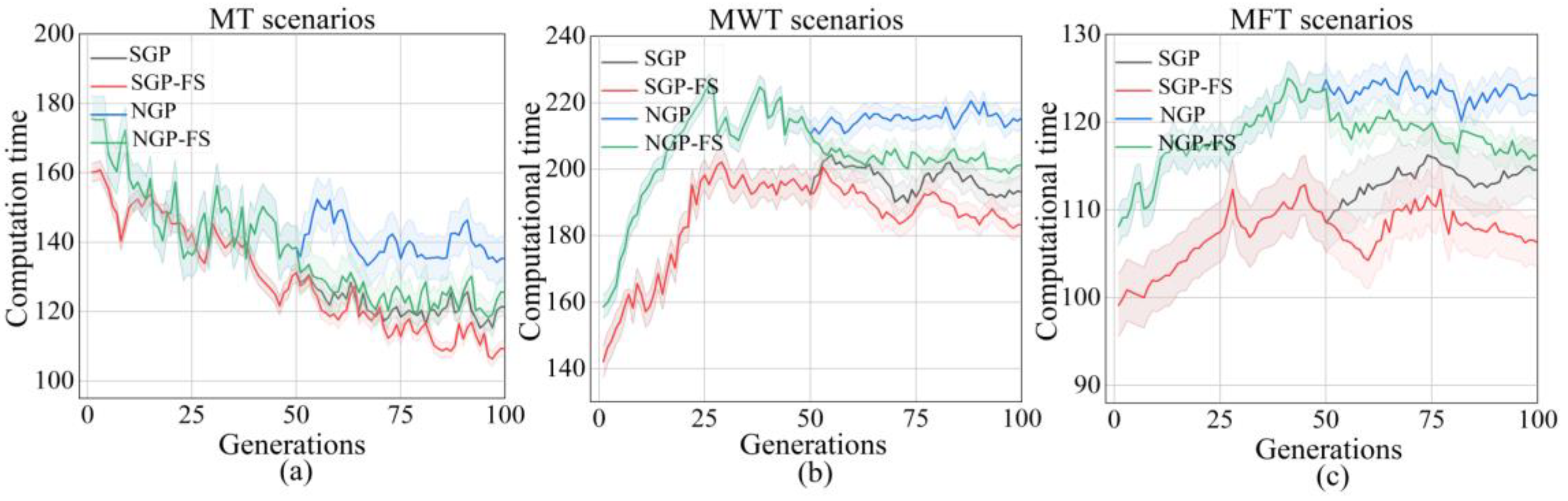
In terms of computational budget, it is clear that the NGP algorithm has the highest computational time than the other algorithm in the three objectives, as shown in Figure 5a–c. The main reason is that the replacement operator requires more individual evaluation. Although the NGP-FS has no advantage in the first 50 generations, it achieved a similar computational time as the SGP and SGP-FS after the feature selection process. This may indicate that, compared with a large feature set, using a limited terminal set with chosen features allows for the development of more effective rules. It is also noted that there is no big difference between the computational time of the SGP and SGP-FS, which indicates that selected features without accuracy cannot decrease the computational time of the algorithm.
Finally, it can be concluded that the NGP-FS algorithm can evolve compact and high-quality dispatching rules in a feasible computational time under different objectives.
5.2. Test Performance
In order to show the effectiveness of the proposed approach, the outcomes of test scenarios for the MT, MWT, and MFT goals are presented in this section. The average results (mean) and standard deviation (std) of the best dispatching rules developed by the four algorithms in 30 different runs for three goals are shown in Table 6, Table 7 and Table 8. Tests also show the objective value of the best benchmarking rules for each scenario. Under the MT objective, the NGP-FS algorithm significantly outperforms the BR, SGP, and SGP-FS algorithms in all simulated scenarios. The MT objective value of NGP-FS varies from 15.57 ± 3.67 (lowest value) to 400.81 ± 10.84 (highest value) in 27 scenarios, as shown in Table 6. In particular, when the scenarios become more complex, the gap between them is more obvious, e.g., the objective value obtained by the best benchmark rule 2PT+ WINQ + NPT is 200% larger than those obtained with rules evolved by NGP-FS in <100, 2, 99%> and <50, 2, 99%> scenarios. The scenarios with significant gaps are shown in bold. Compared with the NGP algorithm, NGP-FS obtained better MT results in 24 scenarios, with no significant difference in 3 scenarios. The rules produced using the SGP-FS algorithm have the worst performance compared to the rules developed by other algorithms and compared benchmark rules.
Regarding the MWT objective, the NGP-FS algorithm obtained the best results compared to other algorithms in all 27 instances. Table 7 shows the MWT objective value of NGP-FS varies from 618.48 ± 14.36 (lowest value) to 3258.24 ± 68.79 (highest value) in 27 scenarios. It is significant to mention that the gap between the performance of the NGP-FS algorithm is much clearer than the others. Especially in extreme scenarios with high shop utilization levels and tight due dates, the results of the NGP-FS algorithm are clearly better than those obtained by the NGP and SGP algorithms. As depicted in Table 7, the significantly better results in 12 challenging scenarios are marked in bold, which means that the NGP-FS can produce competitive rules within the time limit. As expected, the rules developed by SGP-FS still have the worst solution quality than those obtained with the other algorithms in all scenarios.
For the scenarios with MFT as objective, the NGP-FS still has the best objective values (changing from 216.75 ± 3.12 to 759.25 ± 6.19) among the considered methods, as shown in Table 8, but the difference in rule performance is not significant compared to scenarios with MT and MWT objectives. Additionally, the gaps widen in the scenarios with high shop utilization (marked in bold) compared to low utilization scenarios. It is worth noting that changing the tightness factor does not have much of an impact on the job flow time, which is in line with our domain knowledge.
From the experiment results, the following findings can be seen: (1) The benchmark rules achieve higher standard deviations than the GP-based methods in the three aforementioned objectives, which indicates that the manually designed dispatching rules are less robust. More particular, human-made dispatching rules are unable to deliver consistent results under a variety of working circumstances. (2) Further observation of the performance of the rules indicates that the NGP rules are also able to achieve good performance among the considered algorithms. This supports our assertion that the GP diversity management strategy can have an important and favorable influence on the quality of the solutions. (3) The average improvement of the NGP-FS rules over the best-evolved rules by the other three GP-based algorithms is 13.28%, 12.57%, and 15.62% in the mean tardiness (MT), mean flow time (MFT), and mean weighted tardiness (MWT) objective, respectively. (4) Finally, compared with SGP, SGP-FS, NGP, and benchmark rules, the proposed NGP-FS algorithm is able to generate high-quality rules with impressive small sizes in a feasible computational time when dealing with different job shop conditions.
5.3. Unique Feature Analysis
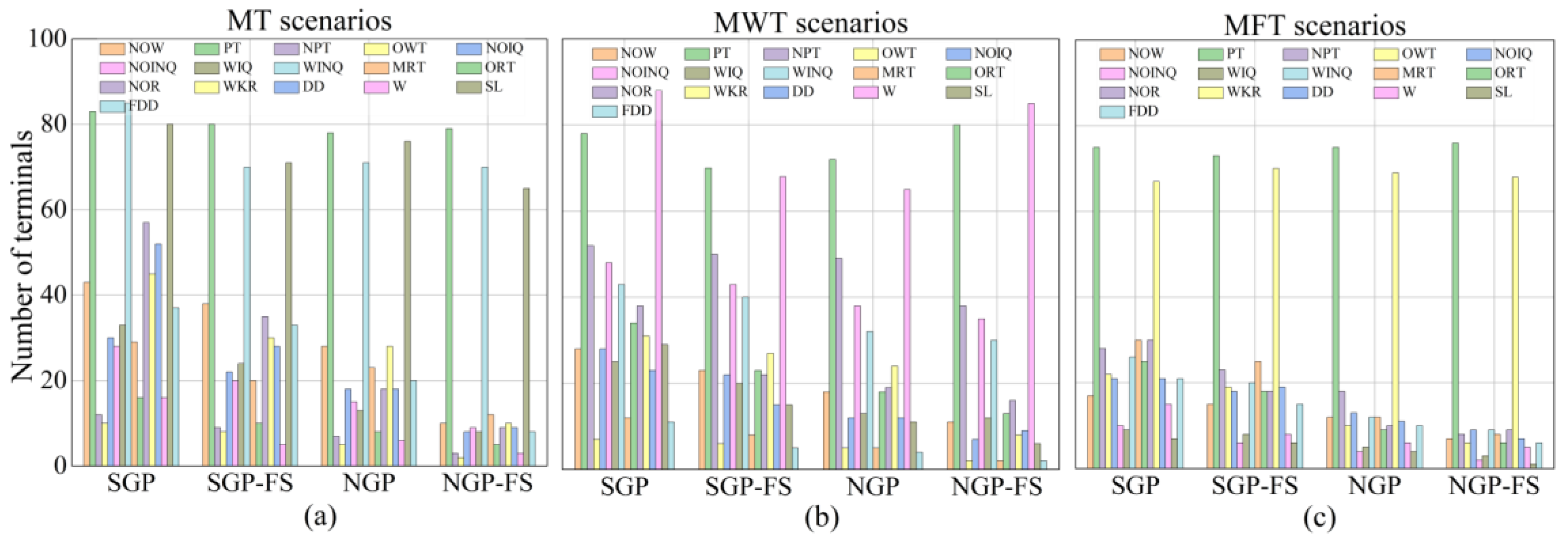
To further verify the superiority of the NGP-FS algorithm in the complexity of generated rules, the number of unique features of the best-evolved rules using SGP, SGP-FS, NGP, and NGP-FS methods is analyzed. Figure 6a–c exhibit the feature distribution of the 30 best-evolved rules in three considered objectives, respectively. It is evident that the created rules have much less unique features than other algorithms, indicating that the NGP-FS algorithm has more potential to achieve smaller rules for interpretation. In addition, the gaps between relevant and irrelevant features are comparatively larger than the other related approaches. For the scenarios with MT as the objective, the NGP-FS rules achieve a reduction in the number of features by 35.75%, 31.26%, and 12.69% compared to SGP, SGP-FS, and NGP methods. Moreover, the most important features, PT, WINQ, NOR, DD, NOW, and WKR, are apparently visualized compared to the unimportant features ORT, OWT, NPT, and W. Regarding the MWT objective, the rules evolved by the NGP-FS algorithm decrease the number of features in best-evolved rules with 38.24%, 29.78%, and 13.35% compared to SGP, SGP-FS, and NGP methods, respectively. The GP-based algorithms choose W as an important feature to minimize mean-weighted tardiness rather than mean tardiness and mean flow time as expected, whereas the MR, OWT, and FDD features are non-significant. As for the MFT objective, the NGP-FS rules have 33.16%, 25.14%, and 15.28% fewer features than the rules produced by the SGP, SGP-FS, and NGP algorithms. The features PT, WKR, and WINQ are included extensively in the best-designed rules of the four algorithms, which indicate that these features have a great impact on minimizing mean flow time.
From the above analysis, it is shown that the proposed approach has the ability to identify the relevant and irrelevant features of the three objective functions. Most importantly, the NGP-FS algorithm shows an outstanding ability to evolve compact and interpretable rules in feasible computational time.
6. Further Analyses
6.1. Feature Analyses
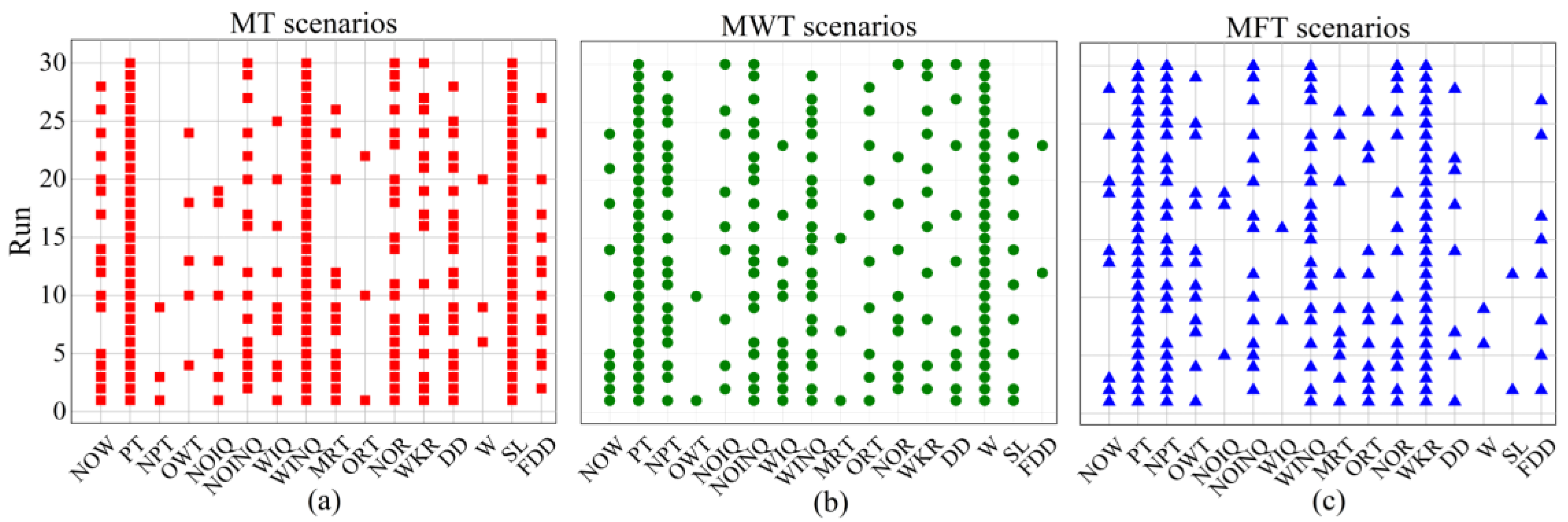
Figure 7a–c exhibit the feature selection results of the NGP-FS algorithm in 30 independent runs for the MT, MWT, and MFT objectives, respectively. Each matrix’s row denotes a run, whereas each column denotes a feature. (Table 2 for details). If a feature is chosen in the th run, a point is drawn at the location where the feature and th run coincide. For the MT objective results depicted in Figure 7a, PT, WINQ, and SL are selected in all 30 runs. It is consistent with the results of previous research [35,37] that PT, WINQ, and SL are the most significant terminals to minimize the mean tardiness. In most runs, NOR, DD, NOW, and WKR features are selected. This means that the jobs with tight due dates and less remaining workload are selected. This means that the jobs with tight due dates and less remaining workload are preferred to be processed in order to reduce the mean tardiness in the job shop. The features ORT, OWT, NPT, and W are not chosen in most runs, which indicates that they may be irrelevant for the MT objective.
As shown in Figure 7b, PT and W are the top significant features to minimize the MWT objective, which aligns with our subject expertise. Expect for these two features, WIQN, NOINQ, and NPT are also selected in most runs, which indicates that the workload information in the next queue is very important to minimizing the MWT objective. In most runs, MRT, OWT, and FDD features are not chosen, which indicates that they have no contribution to the best-evolved rules for the MWT objective. Unlike the findings in early research [5], the feature DD is not included in the irrelevant feature sets, but it is selected more than 40% time. This may be due to the configuration of the experiment, which includes the tight and light due date factor is contained.
For the MFT objective, PT, NPT, WINQ, and WKR play an important role, as depicted in Figure 7c. PT and WKR were selected all over the 30 runs, indicating that the jobs with short processing time and less work remaining have a higher chance of being processed early. WINQ and NPT are selected in most runs, which indicates that the workload information in the next queue is an important factor for the objective of the MFT. However, the features WIQ, NOIQ, SL, and W are rarely selected, which indicates to some extent that these features are irrelevant or redundant in MFT scenarios and may not contribute to the construction of excellent best-evolved rules. Moreover, the importance of the remaining features is not clear.
6.2. Rule Analysis
In order to gain more insight into the rules’ complexity and interpretability, this paper simplifies the rules using the numerical reduction technique mentioned by Nguyen [18]. After the rules have been simplified, they are analyzed on size (number of nodes), depth, and leaves (number of terminals). As it is more challenging to optimize than other objectives, the MWT objective is used as an example. Previous analysis indicates that the NGP-based algorithm has a much larger advantage over the SGP-based algorithm in terms of regular structure. Thus, Equations (13) and (14) show the two example rules obtained by NGP and NGP-FS for further comparison in the MWT objective, respectively. Note that rule 2 has a smaller size than rule 1. Furthermore, rule 2 makes extensive use of useful building blocks like PT/W and WINQ/W, which are well-known to be essential elements for reducing MWT objective value. In contrast, rule 1 still contains features that are not key features (such as NOR, WIQ, and FDD), indicating that the actual part that contributes to the priority function in rule 1 is smaller than that in rule 2. This may be the reason why rule 1 performs worse than rule 2 on training testing. In summary, the proposed NGP-FS approach easily finds more meaningful building blocks than the NGP algorithm through the key feature set.
7. Conclusions and Future Work
The aim of this paper is to analyze if, by using such a combined procedure, it is possible to acquire interpretable and high-quality rules for DJSS automatically. The goal was achieved by integrating a novel GP method, the GP via dynamic diversity management, with feature selection. The novel GP method maintains population diversity using a replacement strategy that combines phenotypic distance-based penalties with a multi-objective Pareto selection based on fitness and simplicity. Then, diverse and promising individuals gained from the novel GP method are used for feature selection to select important terminals. Finally, based on the evolutionary information from the novel GP and selected features, the proposed approach successfully achieved competitive dispatching rules. The proposed approach (NGP-FS) was compared to three algorithms (SGP, SGP-FS, NGP) in MT scenarios, MWT scenarios, and MFT scenarios from the aspect of rule size, solution quality of designed rules, and computation time.
Experimental results show that the proposed approach can design more interpretable and high-quality rules and achieve high robustness to complex scenarios. Considering the distribution of features in the best rules, the NGP-FS obtains compact rules with a small terminal set of selected features. Based on the rule analysis, it reveals that the NGP-FS has the ability to find more meaningful building blocks to improve rule performance. Besides having a compact structure, the NGP-FS evolved rules present overall improvement compared to the rules evolved by the other three algorithms (SGP, SGP-FS, NGP) under three objective functions (MT, MWT, MFT).
As future research, the suggested approach can be extended to develop numerous dispatching rules for a variety of workshop scenarios and dynamically adapt to the shop’s status. These job shop situations might include the arrival of urgent work, machine problems, order cancellations, or lot size adjustments. Furthermore, this work should be tested in different types of job shops, such as flexible job shop scheduling or parallel machine scheduling, while optimizing single or multi-objectives.
Author Contributions
A.S.: Conceptualization, methodology, data curation, formal analysis, validation, writing—original draft, writing—review and editing. Y.Y.: methodology, project administration, supervision. M.L. and J.M.: resources and supervision. Z.B. and Y.L.: methodology and project administration. All authors have read and agreed to the published version of the manuscript.
Funding
This research was funded by the National Natural Science Foundation of China (no. 71961029), the Xinjiang Scientific and Technology Project (no. 2020B02013), and the Xinjiang Scientific and Technology Project (no. 2021B01003).
Institutional Review Board Statement
Not applicable.
Informed Consent Statement
Not applicable.
Data Availability Statement
Not applicable.
Acknowledgments
The authors are grateful to the Xinjiang Digital and Manufacturing Center for the use of SIEMENS Plant Simulation software.
Conflicts of Interest
The authors declare no conflict of interest.
References
- Branke, J.; Nguyen, S.; Pickardt, C.W.; Zhang, M. Automated design of production scheduling heuristics: A review. IEEE Trans. Evol. Comput. 2016, 20, 110–124. [Google Scholar] [CrossRef] [Green Version]
- Zhang, F.; Nguyen, S.; Mei, Y.; Zhang, M. Genetic Programming for Production Scheduling; Springer: Singapore, 2021. [Google Scholar]
- Xiong, H.; Shi, S.; Ren, D.; Hu, J. A survey of job shop scheduling problem: The types and models. Comput. Oper. Res. 2022, 142, 105731. [Google Scholar] [CrossRef]
- Kim, J.G.; Jun, H.B.; Bang, J.Y.; Shin, J.H.; Choi, S.H. Minimizing tardiness penalty costs in job shop scheduling under maximum allowable tardiness. Processes 2020, 8, 1398. [Google Scholar] [CrossRef]
- Ghasemi, A.; Ashoori, A.; Heavey, C. Evolutionary learning based simulation optimization for stochastic job shop scheduling problems. Appl. Soft Comput. 2021, 106, 107309. [Google Scholar] [CrossRef]
- Shady, S.; Kaihara, T.; Fujii, N.; Kokuryo, D. Automatic design of dispatching rules with genetic programming for dynamic job shop scheduling. IFIP Adv. Inf. Commun. Technol. 2020, 591, 399–407. [Google Scholar]
- Burke, E.K.; Gendreau, M.; Hyde, M.; Kendall, G.; Ochoa, G.; Özcan, E.; Qu, R. Hyper-heuristics: A survey of the state of the art. J. Oper. Res. Soc. 2013, 64, 1695–1724. [Google Scholar] [CrossRef] [Green Version]
- Braune, R.; Benda, F.; Doerner, K.F.; Hartl, R.F. A genetic programming learning approach to generate dispatching rules for flexible shop scheduling problems. Int. J. Prod. Econ. 2022, 243, 108342. [Google Scholar] [CrossRef]
- Luo, J.; Vanhoucke, M.; Coelho, J.; Guo, W. An efficient genetic programming approach to design priority rules for resource-constrained project scheduling problem. Expert Syst. Appl. 2022, 198, 116753. [Google Scholar] [CrossRef]
- Zhu, X.; Guo, X.; Wang, W.; Wu, J. A Genetic Programming-Based Iterative Approach for the Integrated Process Planning and Scheduling Problem. IEEE Trans. Autom. Sci. Eng. 2022, 19, 2566–2580. [Google Scholar] [CrossRef]
- Lara-Cárdenas, E.; Sánchez-Díaz, X.; Amaya, I.; Cruz-Duarte, J.M.; Ortiz-Bayliss, J.C. A genetic programming framework for heuristic generation for the job-shop scheduling problem. Adv. Soft Comput. 2020, 12468, 284–295. [Google Scholar]
- Zhang, F.; Mei, Y.; Nguyen, S.; Zhang, M. Importance-Aware Genetic Programming for Automated Scheduling Heuristics Learning in Dynamic Flexible Job Shop Scheduling. In Proceedings of the International Conference on Parallel Problem Solving from Nature, Dortmund, Germany, 10–14 September 2022; pp. 48–62. [Google Scholar]
- Omuya, E.O.; Okeyo, G.O.; Kimwele, M.W. Feature selection for classification using principal component analysis and information gain. Expert Syst. Appl. 2021, 174, 114765. [Google Scholar] [CrossRef]
- Salimpour, S.; Kalbkhani, H.; Seyyedi, S.; Solouk, V. Stockwell transform and semi-supervised feature selection from deep features for classification of BCI signals. Sci. Rep. 2022, 12, 11773. [Google Scholar] [CrossRef]
- Song, X.F.; Zhang, Y.; Gong, D.W.; Gao, X.Z. A fast hybrid feature selection based on correlation-guided clustering and particle swarm optimization for high-dimensional data. IEEE Trans. Cybern. 2021, 52, 9573–9586. [Google Scholar] [CrossRef]
- Vandana, C.P.; Chikkamannur, A.A. Feature selection: An empirical study. Int. J. Eng. Trends Technol. 2021, 69, 165–170. [Google Scholar]
- Friedlander, A.; Neshatian, K.; Zhang, M. Meta-learning and feature ranking using genetic programming for classification: Variable terminal weighting. In Proceedings of the 2011 IEEE Congress of Evolutionary Computation (CEC), New Orleans, LA, USA, 5–8 June 2011; pp. 941–948. [Google Scholar]
- Mei, Y.; Zhang, M.; Nyugen, S. Feature selection in evolving job shop dispatching rules with genetic programming. In Proceedings of the Genetic and Evolutionary Computation Conference 2016, Denver, CO, USA, 20–24 July 2016; pp. 365–372. [Google Scholar]
- Mei, Y.; Nguyen, S.; Xue, B.; Zhang, M. An Efficient Feature Selection Algorithm for Evolving Job Shop Scheduling Rules with Genetic Programming. IEEE Trans. Emerg. Top. Comput. Intell. 2017, 1, 339–353. [Google Scholar] [CrossRef]
- Zhang, F.; Mei, Y.; Nguyen, S.; Zhang, M. Evolving scheduling heuristics via genetic programming with feature selection in dynamic flexible job-shop scheduling. IEEE Trans. Cybern. 2020, 51, 1797–1811. [Google Scholar] [CrossRef] [PubMed]
- Xia, J.; Yan, Y.; Ji, L. Research on control strategy and policy optimal scheduling based on an improved genetic algorithm. Neural Comput. Appl. 2022, 34, 9485–9497. [Google Scholar] [CrossRef]
- Zeiträg, Y.; Figueira, J.R.; Horta, N.; Neves, R. Surrogate-assisted automatic evolving of dispatching rules for multi-objective dynamic job shop scheduling using genetic programming. Expert Syst. Appl. 2022, 209, 118194. [Google Scholar] [CrossRef]
- Rafsanjani, M.K.; Riyahi, M. A new hybrid genetic algorithm for job shop scheduling problem. Int. J. Adv. Intell. Paradig. 2020, 16, 157–171. [Google Scholar] [CrossRef]
- Lee, J.; Perkins, D. A simulated annealing algorithm with a dual perturbation method for clustering. Pattern Recognit. 2021, 112, 107713. [Google Scholar] [CrossRef]
- Yi, N.; Xu, J.; Yan, L.; Huang, L. Task optimization and scheduling of distributed cyber–physical system based on improved ant colony algorithm. Future Gener. Comput. Syst. 2020, 109, 134–148. [Google Scholar] [CrossRef]
- Shady, S.; Kaihara, T.; Fujii, N.; Kokuryo, D. A hyper-heuristic framework using GP for dynamic job shop scheduling problem. In Proceedings of the 64th Annual Conference of the Institute of Systems, Control and Information Engineers, Kobe, Japan, 20–22 May 2020; pp. 248–252. [Google Scholar]
- Liu, L.; Shi, L. Automatic Design of Efficient Heuristics for Two-Stage Hybrid Flow Shop Scheduling. Symmetry 2022, 14, 632. [Google Scholar] [CrossRef]
- Branke, J.; Hildebrandt, T.; Scholz-Reiter, B. Hyper-heuristic evolution of dispatching rules: A comparison of rule representations. Evol. Comput. 2015, 23, 249–277. [Google Scholar] [CrossRef] [PubMed]
- Nguyen, S.; Mei, Y.; Zhang, M. Genetic programming for production scheduling: A survey with a unified framework. Complex Intell. Syst. 2017, 3, 41–66. [Google Scholar] [CrossRef] [Green Version]
- Shady, S.; Kaihara, T.; Fujii, N.; Kokuryo, D. Evolving Dispatching Rules Using Genetic Programming for Multi-objective Dynamic Job Shop Scheduling with Machine Breakdowns. Procedia CIRP 2021, 104, 411–416. [Google Scholar] [CrossRef]
- Wen, X.; Lian, X.; Qian, Y.; Zhang, Y.; Wang, H.; Li, H. Dynamic scheduling method for integrated process planning and scheduling problem with machine fault. Robot. Comput. Integr. Manuf. 2022, 77, 102334. [Google Scholar] [CrossRef]
- Burdett, R.L.; Corry, P.; Eustace, C.; Smith, S. Scheduling pre-emptible tasks with flexible resourcing options and auxiliary resource requirements. Comput. Ind. Eng. 2021, 151, 106939. [Google Scholar] [CrossRef]
- Park, J.; Mei, Y.; Nguyen, S.; Chen, G.; Zhang, M. An investigation of ensemble combination schemes for genetic programming based hyper-heuristic approaches to dynamic job shop scheduling. Appl. Soft Comput. 2018, 63, 72–86. [Google Scholar] [CrossRef]
- Zhou, Y.; Yang, J.J.; Huang, Z. Automatic design of scheduling policies for dynamic flexible job shop scheduling via surrogate-assisted cooperative co-evolution genetic programming. Int. J. Prod. Res. 2020, 58, 561–2580. [Google Scholar] [CrossRef]
- Nguyen, S.; Mei, Y.; Xue, B.; Zhang, M. A hybrid genetic programming algorithm for automated design of dispatching rules. Evol. Comput. 2019, 27, 467–496. [Google Scholar] [CrossRef]
- Shady, S.; Kaihara, T.; Fujii, N.; Kokuryo, D. A novel feature selection for evolving compact dispatching rules using genetic programming for dynamic job shop scheduling. Int. J. Prod. Res. 2022, 60, 4025–4048. [Google Scholar] [CrossRef]
- Shady, S.; Kaihara, T.; Fujii, N.; Kokuryo, D. Feature selection approach for evolving reactive scheduling policies for dynamic job shop scheduling problem using gene expression programming. Int. J. Prod. Res. 2022, 60, 1–24. [Google Scholar] [CrossRef]
- Panda, S.; Mei, Y.; Zhang, M. Simplifying Dispatching Rules in Genetic Programming for Dynamic Job Shop Scheduling. In Proceedings of the European Conference on Evolutionary Computation in Combinatorial Optimization, Madrid, Spain, 20–22 April 2022; pp. 95–110. [Google Scholar]
- Huang, Z.; Zhang, F.; Mei, Y.; Zhang, M. An Investigation of Multitask Linear Genetic Programming for Dynamic Job Shop Scheduling. In Proceedings of the European Conference on Genetic Programming (Part of EvoStar), Madrid, Spain, 20–22 April 2022; pp. 162–178. [Google Scholar]
- Fan, H.; Xiong, H.; Goh, M. Genetic programming-based hyper-heuristic approach for solving dynamic job shop scheduling problem with extended technical precedence constraints. Comput. Oper. Res. 2021, 134, 105401. [Google Scholar] [CrossRef]
- Chen, Q.; Xue, B.; Zhang, M. Preserving population diversity based on transformed semantics in genetic programming for symbolic regression. IEEE Trans. Evol. Comput. 2020, 25, 433–447. [Google Scholar] [CrossRef]
- Rueda, R.; Cuéllar, M.P.; Ruíz LG, B.; Pegalajar, M.C. A similarity measure for Straight Line Programs and its application to control diversity in Genetic Programming. Expert Syst. Appl. 2022, 194, 116415. [Google Scholar] [CrossRef]
- Nieto-Fuentes, R.; Segura, C. GP-DMD: A genetic programming variant with dynamic management of diversity. Genet. Program. Evolvable Mach. 2022, 23, 279–304. [Google Scholar] [CrossRef]
- Zhang, F.; Mei, Y.; Nguyen, S.; Zhang, M.; Tan, K.C. Surrogate-assisted evolutionary multitask genetic programming for dynamic flexible job shop scheduling. IEEE Trans. Evol. Comput. 2021, 25, 651–665. [Google Scholar] [CrossRef]
- Ferreira, C.; Figueira, G.; Amorim, P. Effective and interpretable dispatching rules for dynamic job shops via guided empirical learning. Omega 2022, 111, 102643. [Google Scholar] [CrossRef]
Figure 1.
A GP individual tree example and its corresponding dispatching rule.

Figure 2.
Flowchart of the proposed novel genetic programming with online feature selection.

Figure 3.
The percentage deviation of the GP algorithms for the three objectives in the training stage. (a): Percentage change in MT scenarios across generations, (b): Percentage change in MWT scenarios across generations, and (c): Percentage change in MFT scenarios across generations.
Figure 3.
The percentage deviation of the GP algorithms for the three objectives in the training stage. (a): Percentage change in MT scenarios across generations, (b): Percentage change in MWT scenarios across generations, and (c): Percentage change in MFT scenarios across generations.

Figure 4.
The average rule size of the GP algorithms for the three objectives in the training stage. (a): Mean rule size across generations for the MT scenarios, (b): Mean rule size across generations for the MWT scenarios, and (c): Mean rule size across generations for the MFT scenarios.
Figure 4.
The average rule size of the GP algorithms for the three objectives in the training stage. (a): Mean rule size across generations for the MT scenarios, (b): Mean rule size across generations for the MWT scenarios, and (c): Mean rule size across generations for the MFT scenarios.

Figure 5.
The computational time of the GP algorithms for the three objectives in the training stage. (a): Computational time across generations for the MT scenarios, (b): Computational time across generations for the MWT scenarios, and (c): Computational time across generations for the MFT scenarios.

Figure 6.
Terminal distribution in the 30 best-evolved rules for the SGP, SGP-FS, NGP, and NGP-FS algorithms for the three objectives. (a): Terminal distribution for the MT scenarios, (b): Terminal distribution for the MWT scenarios, and (c): Terminal distribution for the MFT scenarios.
Figure 6.
Terminal distribution in the 30 best-evolved rules for the SGP, SGP-FS, NGP, and NGP-FS algorithms for the three objectives. (a): Terminal distribution for the MT scenarios, (b): Terminal distribution for the MWT scenarios, and (c): Terminal distribution for the MFT scenarios.

Figure 7.
The matrix plot of the feature selection results of the SGP-FS Algorithm for the three objectives. (a): Selected terminals using the SGP-FS algorithm for the MT scenarios, (b): Selected terminals using the SGP-FS algorithm for the MWT scenarios, and (c): Selected terminals using the SGP-FS algorithm for the MFT scenarios.


Table 1.
Scenarios used in simulations for training and testing.
| Parameter | Description | Training | Test |
|---|---|---|---|
| Mean processing time | 25, 50 | 25, 50, 100 | |
| Due dates tightness factor | 3, 5, 7 | 2, 4, 6 | |
| Shop utilization level | 85, 90, 95 | 80, 90, 99, | |
| Scenariosreplications | 181 | 27 | |
| Objectives functions: MT, MWT, MFT, | |||
Table 2.
The GP terminal and function sets.
| Node Name | Description |
|---|---|
| NOW | The current time |
| PT | Processing time of the operation |
| NPT | Processing time of the next operation |
| OWT | The waiting time of the operation |
| NOIQ | Number of operations in the current queue |
| NOINQ | Number of operations in the next queue |
| WIQ | Work in the current queue |
| WINQ | Work in the next queue |
| MRT | Ready time of the machine |
| ORT | Ready time of the operation |
| NOR | Number of operations remaining |
| WKR | Work remaining (including the current operation) |
| DD | Due date of the job |
| W | Weight of the job |
| SL | Slack time of the job |
| FDD | Flow due date of the operation |
| Function set | +,−,×,/, max, min |
Table 3.
Parameter settings.
| Parameter | Value |
|---|---|
| Initialization | Ramped-half-and-half |
| Population size | 450 |
| Maximal depth | 8 |
| Crossover/Mutation rate | 90%/20% |
| Selection | Tournament selection (size = 5) |
| Number of generations in stage 1 and stage 3 | 50/50 |
| Terminal/non-terminal selection rate | 10%/90% |
Table 4.
Benchmark dispatching rules.
| Benchmark Rules | Descriptions |
|---|---|
| SPT | Shortest processing time |
| EDD | Earliest due date |
| FDD | Earliest flow due date |
| LPT | Longest processing time |
| FIFO | First in, first out |
| LILO | Last in, last out |
| CR | Critical ratio |
| RR | Raghu and Rajendran |
| MDD | Modified due date |
| SL | Slack |
| WATC | Weighted apparent tardiness cost |
| COVERT | Cost over time |
| PW | Process waiting time |
| NPT | Next processing time |
| WINQ | Work in next queue |
| PT+WINQ | Processing time+WINQ |
| 2PT+WINQ+NPT | Double processing time+WINQ+NPT |
| PT+WINQ+SL | Processing time+WINQ+SL |
| SPT+PW+FDD | Processing time+PW+FDD |
| 2PT+WINQ+NPT+WSL | 2Processing time+WINQ+NPT+waiting slack |
Table 5.
Mean and standard deviation of the performance measures (training phase).
| Measures | Obj | SGP | SGP-FS | NGP | NGP-FS |
|---|---|---|---|---|---|
| Percentage deviation | MT | 115.78 ± 5.21 | 106.21 ± 12.37 | 126.92 ± 4.25 | 141.58 ± 3.69 (+,+,+) |
| MWT | 131.57 ± 15.23 | 128.18 ± 21.28 | 145.46 ± 12.77 | 162.33 ± 10.97 (+,+,+) | |
| MFT | 78.03 ± 2.91 | 66.14 ± 5.24 | 111.24 ± 3.61 | 119.57 ± 3.58 (+,+,+) | |
| Mean rule size | MT | 25.23 ± 3.35 | 20.85 ± 3.57 | 19.23 ± 3.15 | 17.26 ± 2.67 (+,+,+) |
| MWT | 27.19 ± 4.36 | 25.85 ± 3.49 | 22.23 ± 3.08 | 18.56 ± 2.78 (+,+,+) | |
| MFT | 26.15 ± 3.46 | 21.36 ± 3.81 | 18.23 ± 1.79 | 14.63 ± 1.26 (+,+,+) | |
| Computational time | MT | 131.83 ± 2.67 | 125.66 ± 1.95 | 145.04 ± 6.77 | 132.64 ± 3.14 (+,=,+) |
| MWT | 189.43 ± 4.73 | 180.14 ± 3.91 | 210.18 ± 3.36 | 195.26 ± 3.44 (+,=,+) | |
| MFT | 113.83 ± 3.67 | 110.66 ± 3.95 | 120.04 ± 1.97 | 114.64 ± 2.11 (+,=,+) |
Table 6.
Mean and standard deviation of the MT objective value of the considered algorithms in the testing phase.
Table 6.
Mean and standard deviation of the MT objective value of the considered algorithms in the testing phase.
| Scenarios | RBR | SGP | SGP-FS | NGP | NGP-FS |
|---|---|---|---|---|---|
| (20, 2, 80%) | 56.34 ± 9.97 (PT+WINQ) | 51.78 ± 5.35 | 54.86 ± 2.43 | 48.54 ± 5.69 | 44.88 ± 3.62 (+, +, +, +) |
| (20, 2, 90%) | 148.12 ± 17.45 (PT+WINQ) | 135.84 ± 7.81 | 142.58 ± 4.14 | 128.77 ± 15.46 | 121.56 ± 16.83 (+, +, +, +) |
| (20, 2, 99%) | 204.33 ± 22.01 (PT+WINQ) | 195.36 ± 12.13 | 201.61 ± 18.56 | 145.85 ± 15.27 | 88.60 ± 6.99 (+, +, +, +) |
| (20, 4, 80%) | 87.64 ± 11.79 (PT+WINQ) | 88.67 ± 6.35 | 92.15 ± 9.25 | 86.84 ± 8.49 | 82.93 ± 7.15 (+, +, +, +) |
| (20, 4, 90%) | 120.62 ± 18.19 (2PT+NPT+WINQ) | 121.28 ± 7.59 | 125.69 ± 8.82 | 115.98 ± 17.71 | 116.32 ± 18.56 (+, +, +, =) |
| (20, 4, 99%) | 329.25 ± 16.38 (PT+WINQ) | 322.13 ± 2.3 | 338.15 ± 27.43 | 313.58 ± 20.98 | 314.25 ± 17.92 (+, +, +, =) |
| (20, 6, 80%) | 30.72 ± 19.97 (COVERT) | 22.15 ± 9.92 | 28.60 ± 6.91 | 20.45 ± 15.37 | 16.85 ± 17.92 (+, +, +, +) |
| (20, 6, 90%) | 91.99 ± 14.56 (COVERT) | 90.33 ± 11.01 | 92.15 ± 10.27 | 87.67 ± 15.09 | 85.44 ± 12.63 (+, +, +, =) |
| (20, 6, 99%) | 409.14 ± 25.32(RR) | 409.52 ± 15.55 | 411.24 ± 18.48 | 405.79 ± 12.17 | 400.81 ± 10.84 (+, +, +, +) |
| (50, 2, 80%) | 84.48 ± 21.63 (PT+WINQ) | 83.95 ± 5.69 | 85.89 ± 4.16 | 78.22 ± 7.15 | 75.47 ± 5.89 (+, +, +, +) |
| (50, 2, 90%) | 71.51 ± 14.99 (PT+WINQ) | 69.17 ± 5.88 | 72.29 ± 7.25 | 69.19 ± 3.84 | 65.18 ± 2.97 (+, +, +, +) |
| (50, 2, 99%) | 246.77 ± 62.59 (2PT+NPT+WINQ) | 233.06 ± 19.42 | 255.47 ± 51.92 | 185.12 ± 17.59 | 135.29 ± 18.64 (+, +, +, +) |
| (50, 4, 80%) | 48.98 ± 11.04 (2PT+NPT+WINQ) | 48.61 ± 2.95 | 52.17 ± 8.32 | 38.1 ± 4.09 | 35.74 ± 4.14 (+, +, +, +) |
| (50, 4, 90%) | 303.6 ± 45.68 (COVERT) | 299.65 ± 28.79 | 310.55 ± 35.07 | 287.35 ± 21.22 | 285.16 ± 18.87 (+, +, +, =) |
| (50, 4, 99%) | 57.97 ± 21.25 (SL/RO) | 55.15 ± 9.63 | 65.84 ± 10.16 | 50.63 ± 8.25 | 45.23 ± 9.12 (+, +, +, +) |
| (50, 6, 80%) | 148.89 ± 32.45 (PT+WINQ) | 145.52 ± 15.06 | 156.29 ± 11.81 | 142.87 ± 10.93 | 137.65 ± 16.34 (+, +, +, +) |
| (50, 6, 90%) | 67.11 ± 14.38 (SL/RO) | 68.29 ± 14.43 | 72.37 ± 11.67 | 60.25 ± 12.29 | 54.15 ± 14.15 (+, +, +, +) |
| (50, 6, 99%) | 75.95 ± 14.38 (COVERT) | 74.17 ± 8.88 | 82.16 ± 9.13 | 69.15 ± 7.08 | 64.25 ± 6.89 (+, +, +, +) |
| (100, 2, 80%) | 51.67 ± 7.19 (2PT+NPT+WINQ) | 48.97 ± 5.86 | 53.79 ± 5.39 | 31.18 ± 4.61 | 25.16 ± 3.74 (+, +, +, +) |
| (100, 2, 90%) | 141.25 ± 26.94 (PT+WINQ) | 138.15 ± 17.13 | 145.17 ± 16.99 | 126.48 ± 18.79 | 117.26 ± 17.52 (+, +, +, +) |
| (100, 2, 99%) | 147.37 ± 24.86 (2PT+NPT+WINQ) | 142.38 ± 15.79 | 152.49 ± 28.01 | 105.69 ± 14.21 | 73.45 ± 15.13 (+, +, +, +) |
| (100, 4, 80%) | 30.64 ± 25.71 (PT+WINQ) | 29.32 ± 2.67 | 35.14 ± 9.59 | 22.37 ± 5.89 | 15.57 ± 3.67 (+, +, +, +) |
| (100, 4, 90%) | 242.83 ± 33.71 (COVERT) | 240.18 ± 27.06 | 251.29 ± 28.17 | 229.16 ± 22.40 | 225.84 ± 21.28 (+, +, +, +) |
| (100, 4, 99%) | 301.55 ± 41.79 (PT+WINQ) | 283.67 ± 15.47 | 302.47 ± 24.09 | 162.28 ± 17.13 | 156.42 ± 16.67 (+, +, +, +) |
| (100, 6, 80%) | 227.26 ± 48.99 (COVERT) | 222.81 ± 28.16 | 232.71 ± 38.30 | 211.06 ± 32.95 | 198.08 ± 34.56 (+, +, +, +) |
| (100, 6, 90%) | 198.05 ± 76.56 (COVERT) | 195.78 ± 15.20 | 215.48 ± 26.38 | 187.26 ± 18.81 | 181.47 ± 21.28 (+, +, +, +) |
| (100, 6, 99%) | 42.54 ± 27.48 (COVERT) | 37.85 ± 4.73 | 49.92 ± 13.65 | 34.91 ± 8.29 | 32.45 ± 7.59 (+, +, +, +) |
Table 7.
Mean and standard deviation of the MWT objective value of the considered algorithms in the testing phase.
Table 7.
Mean and standard deviation of the MWT objective value of the considered algorithms in the testing phase.
| Scenarios | RBR | SGP | SGP-FS | NGP | NGP-FS |
|---|---|---|---|---|---|
| (20, 2, 80%) | 1583.27 ± 85.48 (WATC) | 1526.94 ± 87.61 | 1694.65 ± 121.26 | 1489 ± 99.34 | 1146.48 ± 71.27 (+, +, +, +) |
| (20, 2, 90%) | 1889.42 ± 78.99 (WATC) | 1874.36 ± 88.34 | 1983.19 ± 112.75 | 1764.22 ± 95.57 | 1609.45 ± 57.31 (+, +, +, +) |
| (20, 2, 99%) | 1914.32 ± 78.31 (WATC) | 1904.53 ± 85.14 | 1935.96 ± 103.67 | 1837.29 ± 95.28 | 1615.84 ± 13.07 (+, +, +, +) |
| (20, 4, 80%) | 2187.37 ± 35.98 (PT+WINQ) | 2199.39 ± 38.73 | 2213.47 ± 45.31 | 2116.48 ± 35.16 | 1959.24 ± 46.63 (+, +, +, +) |
| (20, 4, 90%) | 2796.24 ± 19.58 (2PT+NPT+WINQ) | 2834.07 ± 22.15 | 2867.89 ± 24.14 | 2791.34 ± 20.36 | 2579.85 ± 27.61 (+, +, +, +) |
| (20, 4, 99%) | 948.76 ± 27.48 (PT+WINQ) | 951.93 ± 21.95 | 995.15 ± 26.31 | 927.64 ± 35.18 | 785.34 ± 26.18 (+, +, +, +) |
| (20, 6, 80%) | 1489.76 ± 23.79 (COVERT) | 1507.38 ± 27.13 | 1535.07 ± 38.95 | 1465.67 ± 25.37 | 1237.85 ± 17.92 (+, +, +, +) |
| (20, 6, 90%) | 3637.95 ± 48.99 (COVERT) | 3625.11 ± 55.38 | 3637.59 ± 65.57 | 3512.48 ± 79.05 | 3258.24 ± 68.79 (+, +, +, +) |
| (20, 6, 99%) | 1796.61 ± 16.47(RR) | 1783.29 ± 11.23 | 1899.82 ± 17.89 | 1727.33 ± 9.34 | 1432.11 ± 7.95 (+, +, +, +) |
| (50, 2, 80%) | 1484.68 ± 16.87 (PT+WINQ) | 1413.21 ± 15.06 | 1485.29 ± 24.61 | 1378.52 ± 17.65 | 957.39 ± 15.24 (+, +, +, +) |
| (50, 2, 90%) | 1768.52 ± 24.19 (PT+WINQ) | 1769.37 ± 25.48 | 1872.94 ± 47.58 | 1699.31 ± 23.57 | 1575.28 ± 12.96 (+, +, +, +) |
| (50, 2, 99%) | 2395.77 ± 18.59 (2PT+NPT+WINQ) | 2395.56 ± 39.71 | 2428.27 ± 41.82 | 2385.52 ± 27.65 | 1835.56 ± 19.24 (+, +, +, +) |
| (50, 4, 80%) | 1548.98 ± 21.44 (2PT+NPT+WINQ) | 1597.61 ± 22.64 | 1682.17 ± 28.26 | 1538.1 ± 24.19 | 1335.64 ± 24.24 (+, +, +, +) |
| (50, 4, 90%) | 1524.67 ± 32.78 (COVERT) | 1529.53 ± 38.79 | 1580.28 ± 35.17 | 1487.55 ± 31.72 | 1285.47 ± 28.87 (+, +, +, +) |
| (50, 4, 99%) | 1256.97 ± 19.34 (SL/RO) | 1255.15 ± 19.63 | 1267.74 ± 21.26 | 1150.67 ± 18.25 | 945.73 ± 19.32 (+, +, +, +) |
| (50, 6, 80%) | 1643.89 ± 12.35 (PT+WINQ) | 1605.12 ± 15.27 | 1658.29 ± 18.58 | 1599.28 ± 13.83 | 1137.45 ± 15.62 (+, +, +, +) |
| (50, 6, 90%) | 1667.31 ± 34.38 (SL/RO) | 1660.37 ± 34.83 | 1665.37 ± 32.67 | 1560.25 ± 22.69 | 1454.15 ± 24.35 (+, +, +, +) |
| (50, 6, 99%) | 972.59 ± 14.83 (COVERT) | 989.37 ± 15.28 | 1082.16 ± 11.13 | 969.45 ± 6.27 | 689.25 ± 8.89 (+, +, +, +) |
| (100, 2, 80%) | 1651.37 ± 17.28 (2PT+NPT+WINQ) | 1648.26 ± 15.39 | 1686.81 ± 15.29 | 1531.48 ± 24.61 | 1225.86 ± 23.84 (+, +, +, +) |
| (100, 2, 90%) | 1526.75 ± 26.18 (PT+WINQ) | 1518.15 ± 27.13 | 1545.27 ± 26.99 | 1326.34 ± 28.81 | 1117.26 ± 27.52 (+, +, +, +) |
| (100, 2, 99%) | 1466.67 ± 14.96 (2PT+NPT+WINQ) | 1452.68 ± 17.89 | 1487.59 ± 18.21 | 1385.71 ± 14.21 | 983.65 ± 9.13 (+, +, +, +) |
| (100, 4, 80%) | 2030.64 ± 25.61 (PT+WINQ) | 2029.32 ± 22.35 | 2135.74 ± 29.59 | 1982.77 ± 25.15 | 1715.57 ± 23.67 (+, +, +, +) |
| (100, 4, 90%) | 2442.83 ± 53.92 (COVERT) | 2483.58 ± 57.06 | 2541.29 ± 58.47 | 2429.56 ± 42.47 | 2285.95 ± 41.18 (+, +, +, +) |
| (100, 4, 99%) | 2519.55 ± 33.37 (PT+WINQ) | 2513.17 ± 35.28 | 2598.37 ± 34.29 | 2409.78 ± 37.53 | 2156.42 ± 36.87 (+, +, +, +) |
| (100, 6, 80%) | 927.16 ± 16.05 (COVERT) | 928.81 ± 18.26 | 999.87 ± 18.27 | 911.26 ± 12.96 | 618.48 ± 14.36 (+, +, +, +) |
| (100, 6, 90%) | 1798.25 ± 27.17 (COVERT) | 1795.78 ± 25.19 | 1815.48 ± 27.38 | 1687.26 ± 19.71 | 1481.47 ± 11.28 (+, +, +, +) |
| (100, 6, 99%) | 2022.54 ± 37.56 (COVERT) | 2017.85 ± 34.73 | 2249.92 ± 33.74 | 1934.91 ± 28.29 | 1632.55 ± 17.29 (+, +, +, +) |
Table 8.
Mean and standard deviation of the MFT objective value of the considered algorithms in the testing phase.
Table 8.
Mean and standard deviation of the MFT objective value of the considered algorithms in the testing phase.
| Scenarios | RBR | SGP | SGP-FS | NGP | NGP-FS |
|---|---|---|---|---|---|
| (20, 2, 80%) | 311.21 ± 9.45 (PT+WINQ) | 305.74 ± 3.07 | 309.27 ± 3.14 | 301.35 ± 2.37 | 285.56 ± 1.84 (+, +, +, +) |
| (20, 2, 90%) | 341.89 ± 11.17 (PT+WINQ) | 336.68 ± 4.69 | 339.56 ± 5.27 | 331.63 ± 4.21 | 321.18 ± 2.12 (+, +, +, +) |
| (20, 2, 99%) | 377.33 ± 12.01 (PT+WINQ) | 375.68 ± 5.24 | 371.61 ± 5.49 | 365.27 ± 4.78 | 338.25 ± 4.38 (+, +, +, +) |
| (20, 4, 80%) | 294.64 ± 8.19 (2PT+NPT+WINQ | 288.67 ± 5.67 | 292.25 ± 5.16 | 286.63 ± 3.48 | 281.83 ± 3.27 (+, +, +, +) |
| (20, 4, 90%) | 331.62 ± 10.86 (PT+WINQ) | 324.18 ± 5.32 | 327.69 ± 8.91 | 321.37 ± 7.65 | 315.42 ± 7.78 (+, +, +, +) |
| (20, 4, 99%) | 398.75 ± 15.38 (PT+WINQ) | 389.53 ± 7.13 | 394.34 ± 6.13 | 387.26 ± 5.17 | 365.37 ± 4.19 (+, +, +, +) |
| (20, 6, 80%) | 230.52 ± 13.97 (PT+WINQ) | 225.15 ± 4.96 | 228.60 ± 5.18 | 223.75 ± 3.78 | 216.75 ± 3.12 (+, +, +, +) |
| (20, 6, 90%) | 305.79 ± 14.28 (PT+WINQ) | 296.33 ± 11.01 | 301.75 ± 5.37 | 294.67 ± 4.15 | 285.84 ± 2.47 (+, +, +, +) |
| (20, 6, 99%) | 513.84 ± 28.76 (PT+WINQ) | 509.52 ± 6.35 | 511.34 ± 8.48 | 495.67 ± 5.17 | 456.21 ± 4.23 (+, +, +, +) |
| (50, 2, 80%) | 351.28 ± 12.64 (PT+WINQ) | 341.05 ± 5.23 | 347.69 ± 5.99 | 335.12 ± 5.15 | 325.26 ± 4.16 (+, +, +, +) |
| (50, 2, 90%) | 489.72 ± 17.05 (PT+WINQ) | 478.23 ± 3.57 | 485.49 ± 5.25 | 473.19 ± 2.74 | 465.38 ± 1.97 (+, +, +, +) |
| (50, 2, 99%) | 595.27 ± 37.23 (2PT+NPT+WINQ) | 587.36 ± 4.89 | 591.21 ± 4.12 | 585.12 ± 3.37 | 535.18 ± 2.37 (+, +, +, +) |
| (50, 4, 80%) | 407.98 ± 45.24 (2PT+NPT+WINQ) | 398.26 ± 4.95 | 405.23 ± 4.17 | 395.15 ± 3.94 | 386.69 ± 3.81 (+, +, +, +) |
| (50, 4, 90%) | 431.16 ± 48.28 (PT+WINQ) | 425.15 ± 3.79 | 428.15 ± 5.08 | 421.67 ± 3.88 | 412.66 ± 3.79 (+, +, +, +) |
| (50, 4, 99%) | 617.57 ± 59.25 (PT+WINQ) | 604.27 ± 9.73 | 615.24 ± 10.16 | 591.23 ± 7.13 | 525.73 ± 6.12 (+, +, +, +) |
| (50, 6, 80%) | 358.19 ± 13.79 (PT+WINQ) | 348.12 ± 6.06 | 356.29 ± 8.81 | 345.81 ± 5.92 | 337.25 ± 5.14 (+, +, +, +) |
| (50, 6, 90%) | 497.11 ± 31.67 (PT+WINQ) | 492.29 ± 14.43 | 496.17 ± 9.23 | 485.36 ± 7.19 | 474.37 ± 6.28 (+, +, +, +) |
| (50, 6, 99%) | 695.05 ± 67.36 (PT+WINQ) | 689.37 ± 6.98 | 693.26 ± 7.27 | 686.35 ± 5.98 | 608.48 ± 5.12 (+, +, +, +) |
| (100, 2, 80%) | 451.27 ± 45.48 (2PT+NPT+WINQ) | 444.21 ± 6.17 | 453.29 ± 6.38 | 436.18 ± 5.62 | 425.86 ± 4.74 (+, +, +, +) |
| (100, 2, 90%) | 641.25 ± 56.74 (PT+WINQ) | 632.15 ± 7.05 | 638.67 ± 7.99 | 626.48 ± 6.73 | 618.36 ± 5.77 (+, +, +, +) |
| (100, 2, 99%) | 832.17 ± 85.86 (2PT+NPT+WINQ) | 812.38 ± 5.99 | 826.19 ± 6.01 | 798.27 ± 5.32 | 713.25 ± 4.84 (+, +, +, +) |
| (100, 4, 80%) | 439.24 ± 48.76 (PT+WINQ) | 429.12 ± 6.67 | 435.24 ± 7.27 | 422.27 ± 6.19 | 415.28 ± 5.16 (+, +, +, +) |
| (100, 4, 90%) | 553.83 ± 62.71 (2PT+NPT+WINQ) | 546.18 ± 7.08 | 551.29 ± 8.23 | 539.26 ± 7.12 | 527.34 ± 6.18 (+, +, +, +) |
| (100, 4, 99%) | 815.75 ± 91.87 (PT+WINQ) | 808.27 ± 9.26 | 812.47 ± 10.09 | 804.28 ± 9.58 | 756.12 ± 8.12 (+, +, +, +) |
| (100, 6, 80%) | 537.26 ± 76.19 (PT+WINQ) | 528.71 ± 8.09 | 532.61 ± 8.31 | 521.76 ± 7.25 | 498.58 ± 6.76 (+, +, +, +) |
| (100, 6, 90%) | 668.25 ± 87.56 (PT+WINQ) | 661.78 ± 15.20 | 665.48 ± 26.38 | 657.26 ± 8.19 | 625.17 ± 7.13 (+, +, +, +) |
| (100, 6, 99%) | 852.54 ± 101.27 (PT+WINQ) | 836.75 ± 7.93 | 849.92 ± 8.15 | 824.11 ± 7.72 | 759.25 ± 6.19 (+, +, +, +) |
Disclaimer/Publisher’s Note: The statements, opinions and data contained in all publications are solely those of the individual author(s) and contributor(s) and not of MDPI and/or the editor(s). MDPI and/or the editor(s) disclaim responsibility for any injury to people or property resulting from any ideas, methods, instructions or products referred to in the content. |
© 2022 by the authors. Licensee MDPI, Basel, Switzerland. This article is an open access article distributed under the terms and conditions of the Creative Commons Attribution (CC BY) license (https://creativecommons.org/licenses/by/4.0/).
Share and Cite
MDPI and ACS Style
Sitahong, A.; Yuan, Y.; Li, M.; Ma, J.; Ba, Z.; Lu, Y. Designing Dispatching Rules via Novel Genetic Programming with Feature Selection in Dynamic Job-Shop Scheduling. Processes 2023, 11, 65. https://doi.org/10.3390/pr11010065
AMA Style
Sitahong A, Yuan Y, Li M, Ma J, Ba Z, Lu Y. Designing Dispatching Rules via Novel Genetic Programming with Feature Selection in Dynamic Job-Shop Scheduling. Processes. 2023; 11(1):65. https://doi.org/10.3390/pr11010065
Chicago/Turabian StyleSitahong, Adilanmu, Yiping Yuan, Ming Li, Junyan Ma, Zhiyong Ba, and Yongxin Lu. 2023. "Designing Dispatching Rules via Novel Genetic Programming with Feature Selection in Dynamic Job-Shop Scheduling" Processes 11, no. 1: 65. https://doi.org/10.3390/pr11010065
Note that from the first issue of 2016, this journal uses article numbers instead of page numbers. See further details here.