

Path Planning of Mobile Robots Based on an Improved Particle Swarm Optimization Algorithm
Abstract
:1. Introduction
2. Related Work
3. Principles of PSO and DE
3.1. Particle Swarm Optimization (PSO)
3.2. Differential Evolution Algorithm (DE)
- Establish the initial population and initialize the parameters:
- 2.
- Mutation operation:
- 3.
- Cross operation:
- 4.
- Select operation.
4. Algorithm Improvement
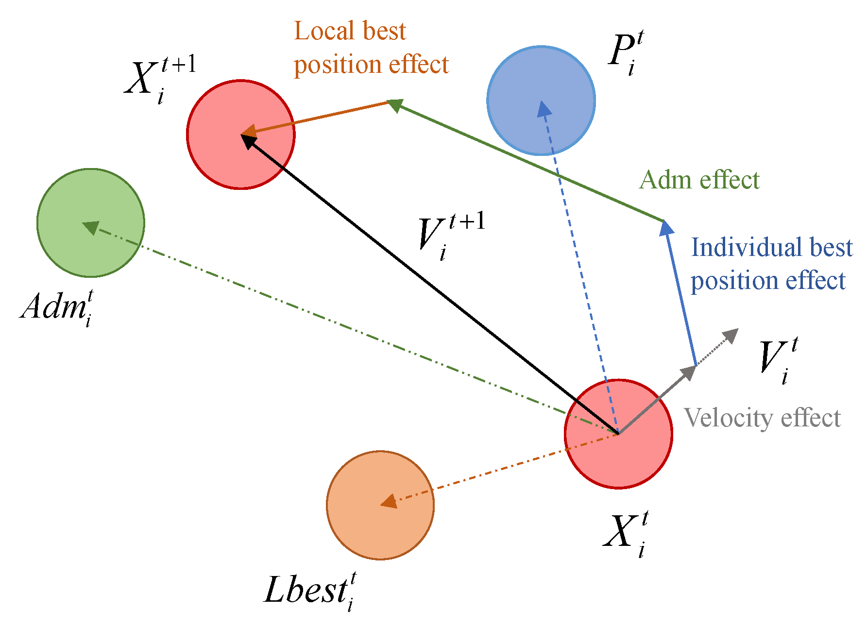
4.1. Improved Particle Swarm Optimization Based on Corporate Governance Idea (IPSO)
- 1.
- 2.
- 3.
- 4.
- 5.
- The improved mathematical formula of pos.ition update formula
4.2. Improved Differential Evolution Algorithm Based on Adaptive Parameters
- Adaptive optimization of scaling factor F
- 2.
- Adaptive optimization of cross probability factor CR
4.3. Hybrid IPSO with IDE (IPSO-IDE)
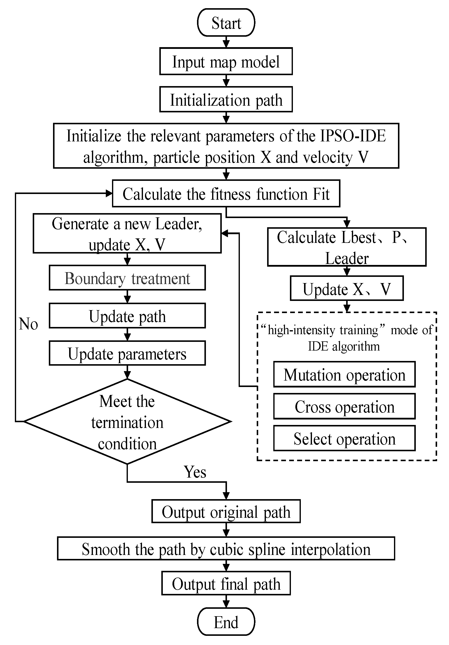
4.3.1. The Principle of IPSO-IDE Algorithm
- step1:
- Initialization parameters, including acceleration factor, number of support votes Opvote, and number of negative votes Owvote, etc.
- step2:
- Initialize the particle swarm randomly, including dimension D, number of population particle N, position X, velocity V, etc.
- step3:
- Calculate the particle fitness value Fit according to the set objective function.
- step4:
- Based on the fitness value Fit, calculate the individual best position Pit, the local best position Lbestit, and elect Adm according to (12) to obtain the global best position.
- step5:
- Update position X and velocity V according to the improved (9) (10) to generate the elite population with high quality.
- step6:
- Use (13) to process the boundary.
- step7:
- Use the elite population as the initial population of IDE, combine the adaptive parameters (14) (15), and use (6) (7) (8) to perform “high intensity” iterative optimization.
- step8:
- Apply the optimized result of IDE algorithm to Leader of the updated particle swarm.
- step9:
- If the termination condition is met, stop the algorithm and output the optimal results. Otherwise, go to Step2.
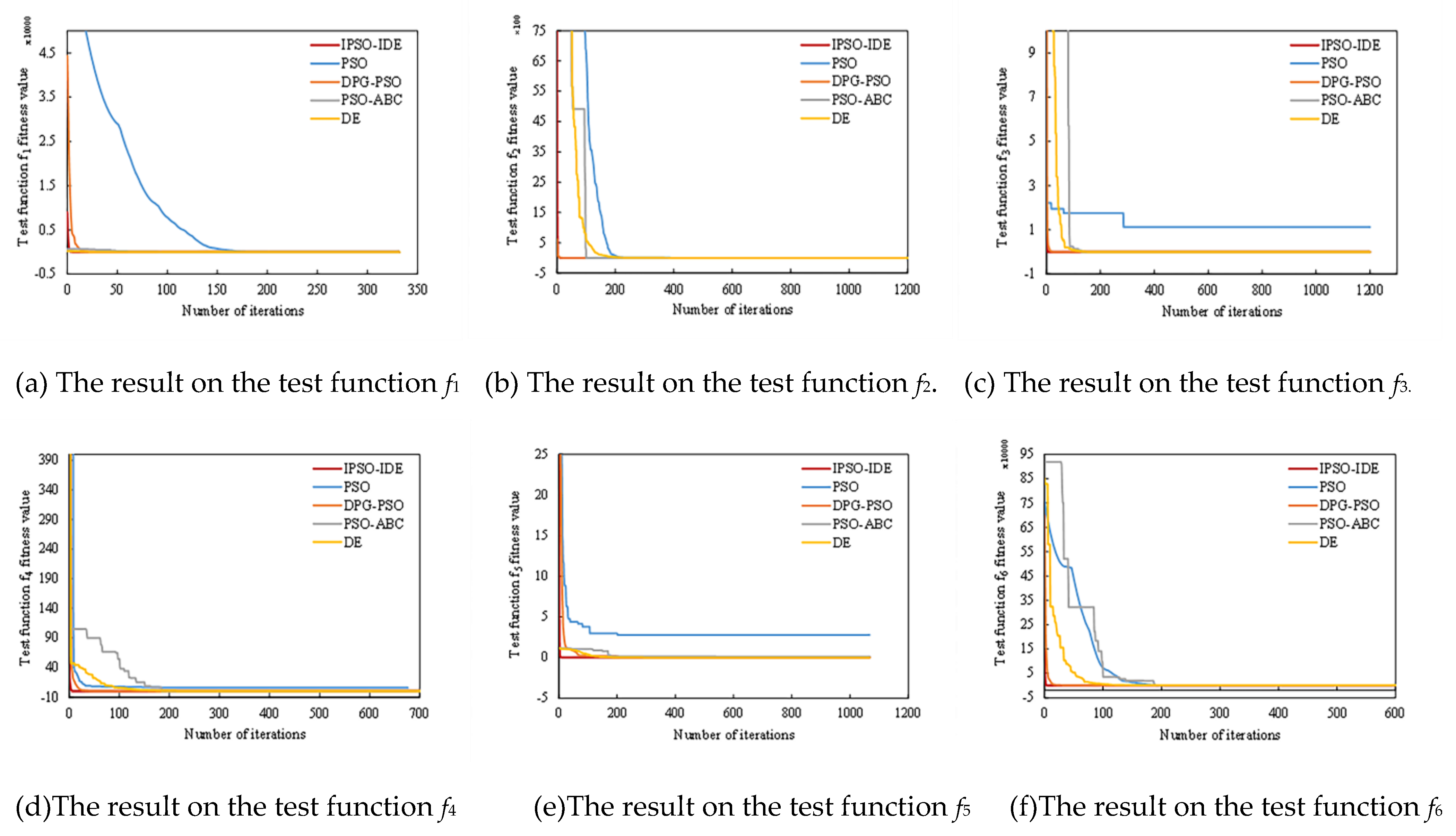
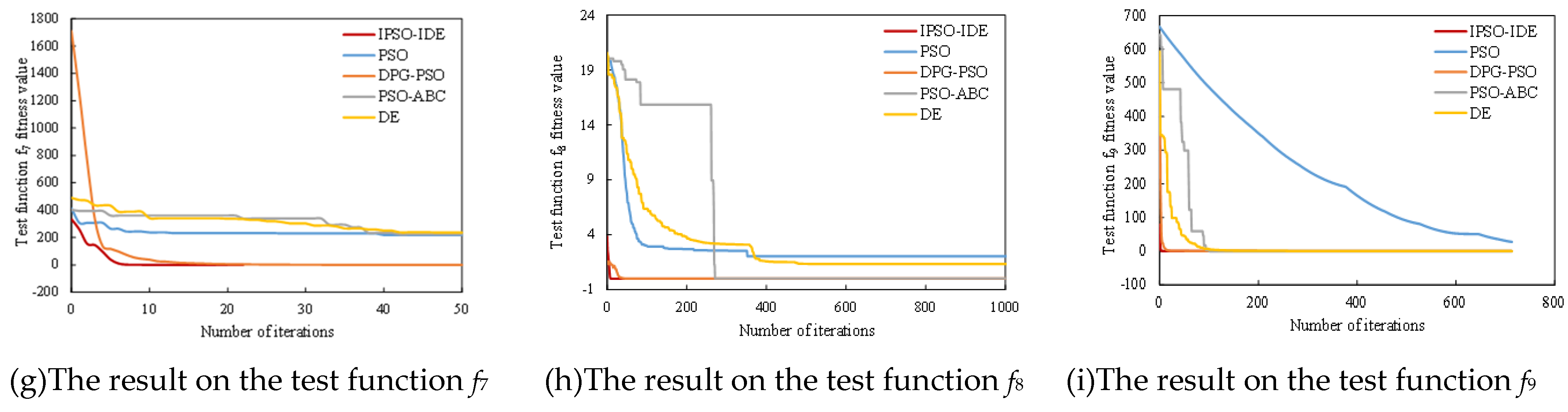
4.3.2. Experimental Verification of IPSO-IDE Model
5. Path Planning Based on IPSO-IDE Algorithm
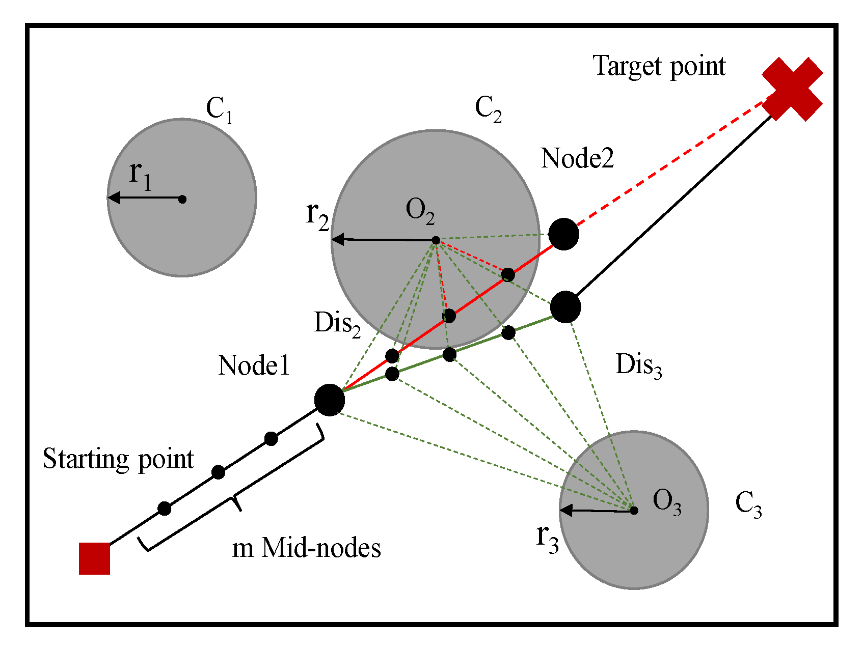
5.1. Design of Fitness Function
- Path length function
- 2.
- Penalty function
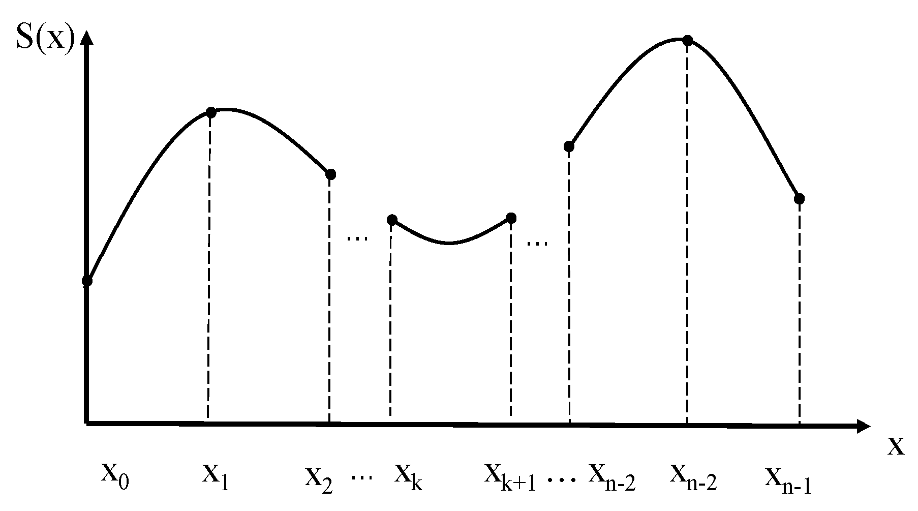
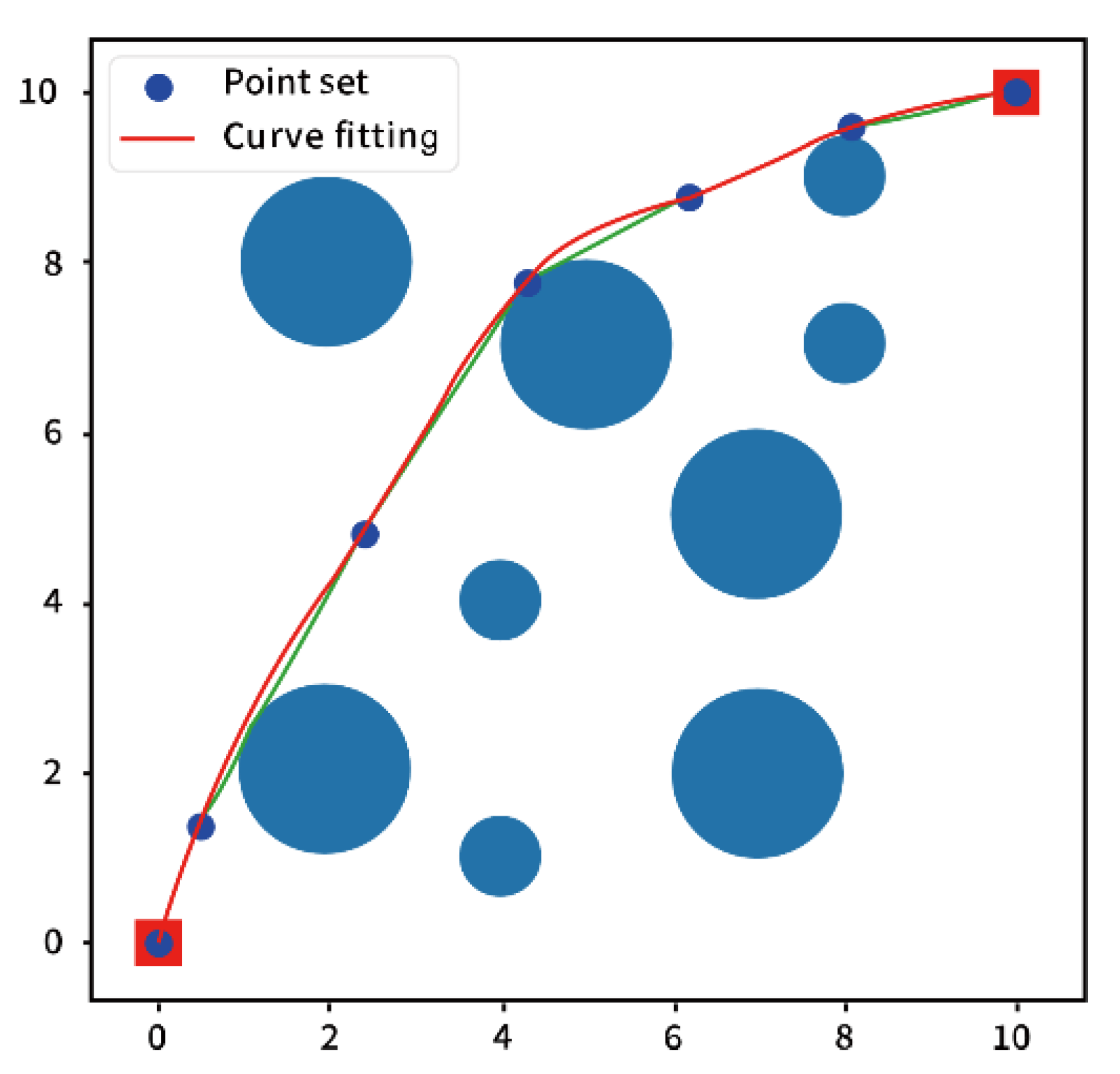
5.2. Path Smoothing
- Basic principle of cubic spline interpolation
- In n subintervals [xi, xi+1] (i = 0, 1, …, n − 1), S(x) is a cubic polynomial.
- S(xi) = yi (i = 0, 1, 2, …, n − 1).
- The first derivative and the second derivative of S(x) in the interval [xmin, xmax] are continuous.
- 2.
- Determine the equation of Spline Interpolation
- According to S(x), which is composed of n cubic polynomials, the polynomial expression can be obtained as:
- According to , it can be concluded that:
- According to the continuity of the differential, it can be concluded that:
- 3.
- Smoothing by spline interpolation
6. Simulation Experiments and Analysis
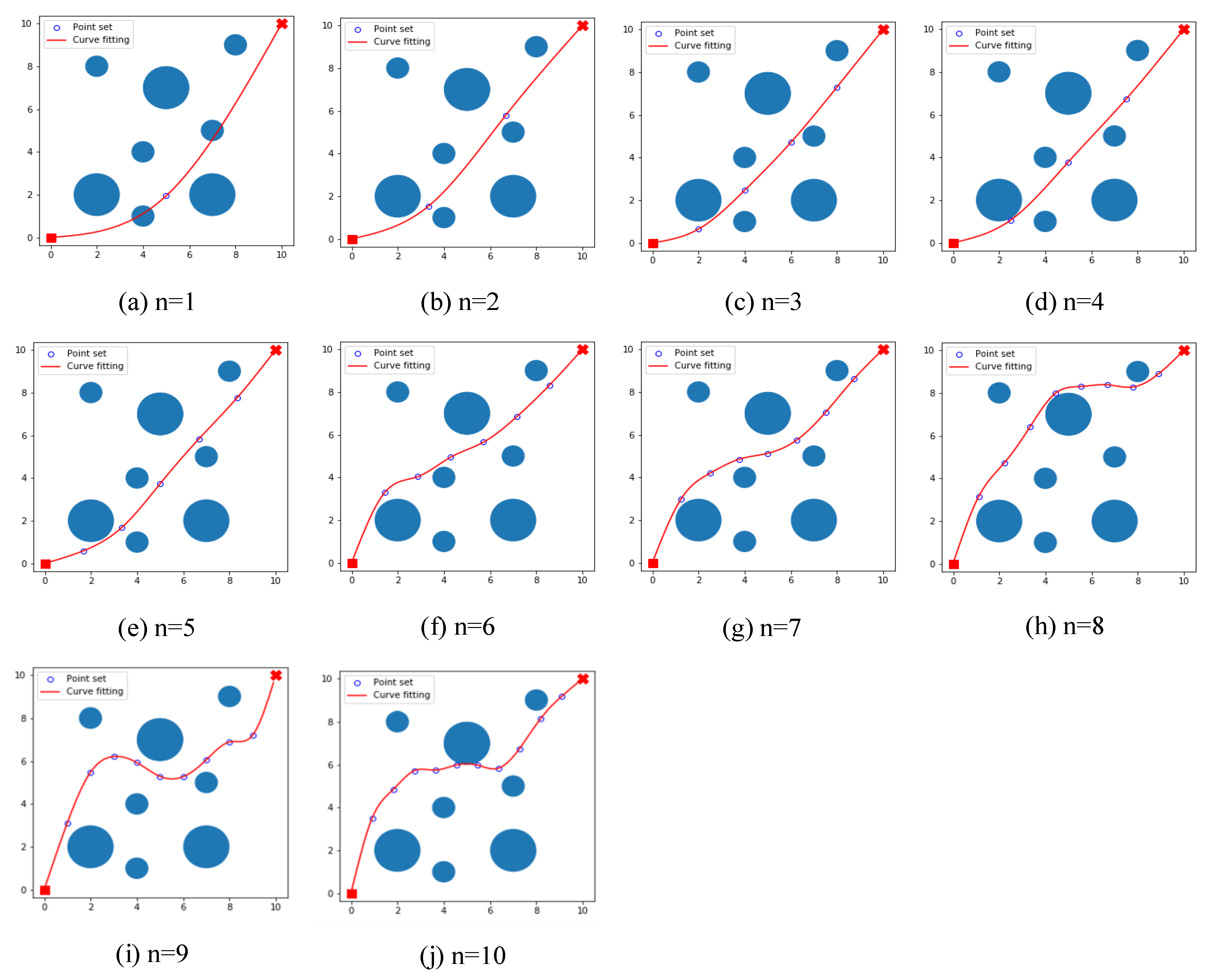
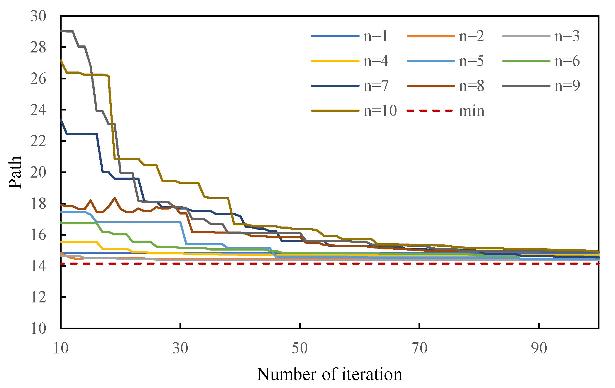
6.1. The Number of Path Nodes Experiment
6.2. Path Planning Experiment
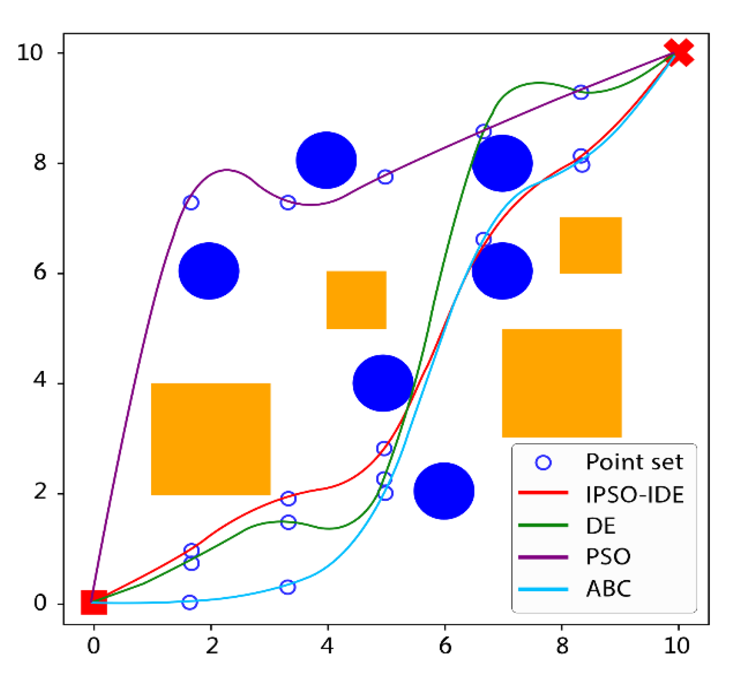
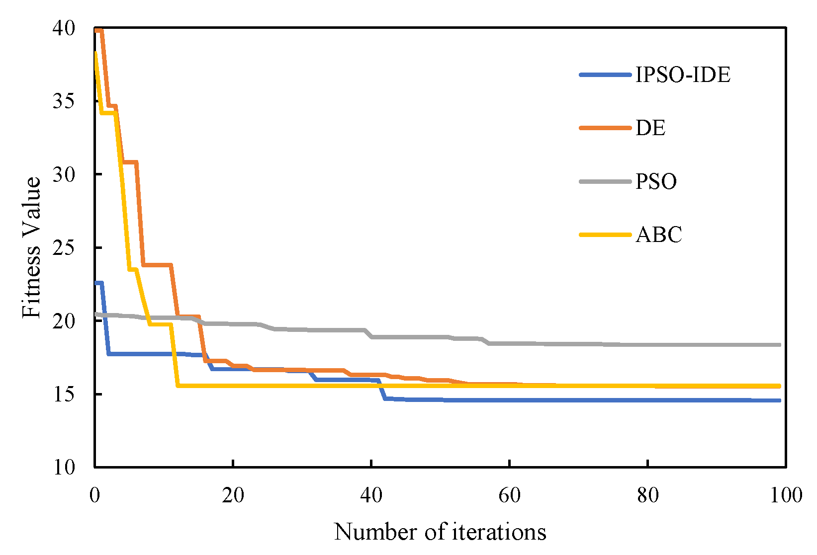
6.2.1. First Experiment: Compared with Different Traditional Heuristic Algorithms
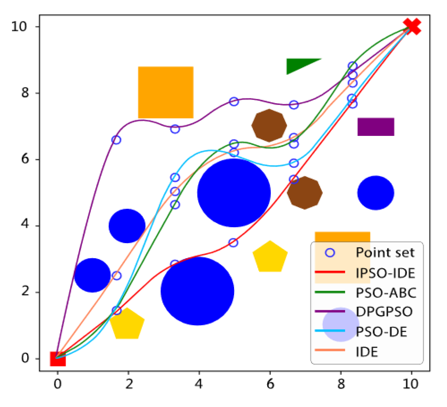
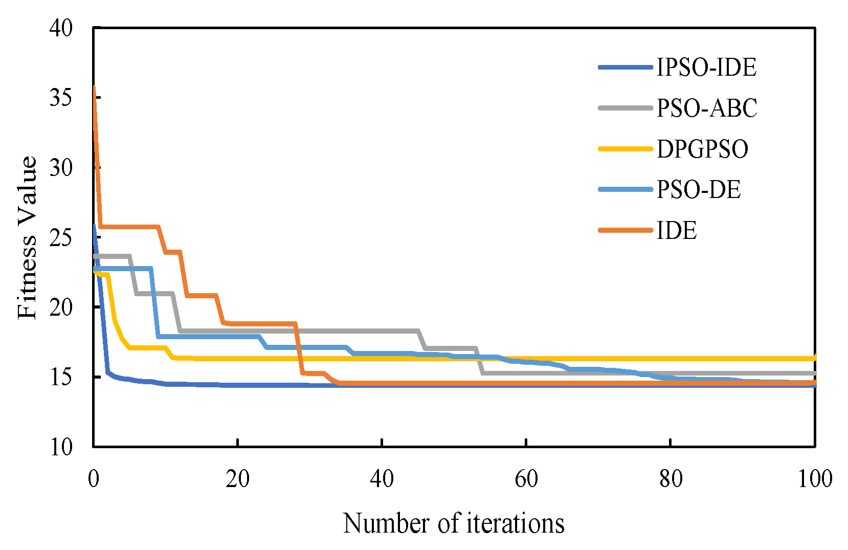
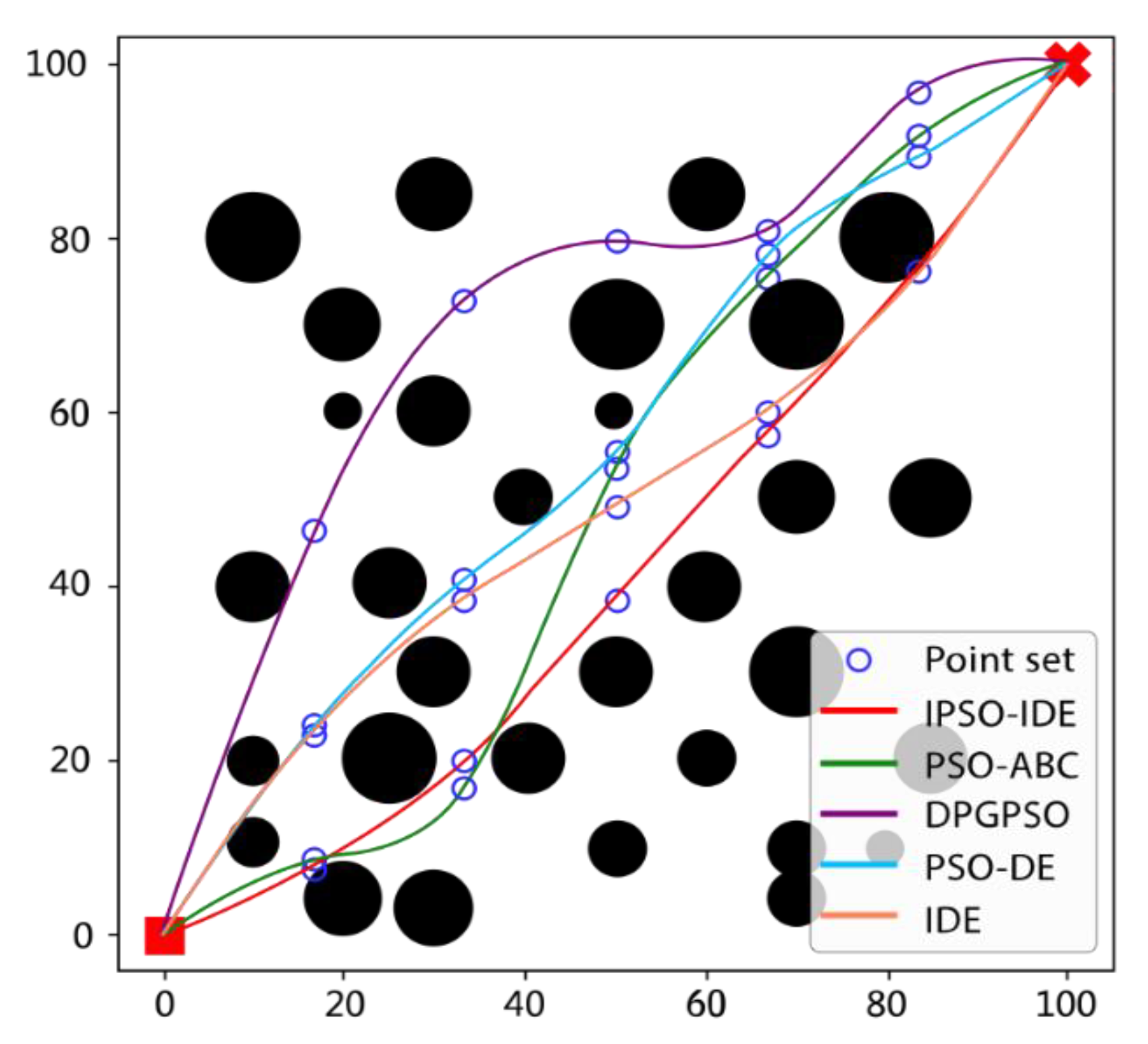
6.2.2. Second Experiment: Compared with Different Improved Algorithms
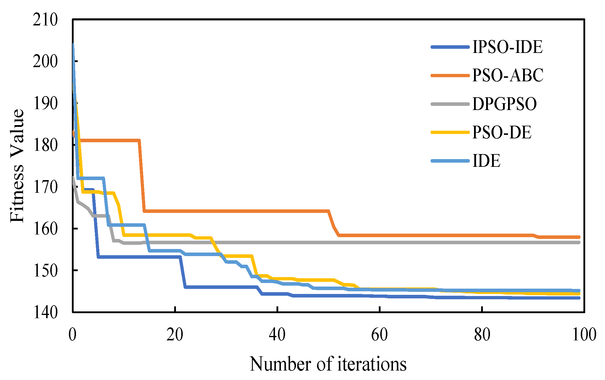
6.2.3. Third Experiment: Verification of Big Map
7. Conclusions
Author Contributions
Funding
Institutional Review Board Statement
Data Availability Statement
Acknowledgments
Conflicts of Interest
Abbreviations
| Abbreviation | meaning |
| PSO | particle swarm optimization |
| IPSO | improved particle swarm optimization |
| DE | differential evolution |
| IDE | optimized differential evolution |
| IPSO- IDE | improved particle swarm optimization based on differential evolution |
| GA | genetic algorithm |
| CR | crossover probability factor |
| DPG-PSO | democracy-inspired particle swarm optimizer with the concept of peer groups |
| ABC | artificial bee colony |
| PSO-ABC | hybrid algorithm based on PSO and ABC |
| Algorithm 1: Code for manager selects |
| //Initialize operator, Owner, operator vote, manager vote, administrator particle. |
| ,voteid: [0,1]. |
|
1.While (fit > fitmin) 2. For t = 1 to T //T is the number of iterations. 3. For i = 1 to N //N is the number of particles in the population. 4. For d = 1 to D //D for dimension. 5. If (voteid < Opvote) 6. //If the particles vote for the operator. 7. Opvote ← Opvote + 1/(M.N) //Add up the votes. 8. Opvote ← Opvote/(Opvote+Owvote) //Standardize voting. 9. Else 10. //If the particle votes for the owner. 11. Owvote ← Owvote + 1/(M.N) //Add up the votes. 12. Owvote←Owvote/(Opvote+Owvote) //Standardize voting. 13. End if 14. expressed as follows. 15. ) 16. ←1 17. End if 18. ) 19. ←2.3 20. End if 21. and Vt 22. End for 23. End for 24.End while |
| Algorithm2: Code for IPSO-IDE |
| Initialize: pro = 1/N, ϕ ← 0.7, Opvote: = ϕ, ovote: = 1− ϕ, |
| c1 ← 0.5, c2 ← 0.5, c3 ← 1.2, c4 ← 1, X, V, Operator, Owner, Leader, Lbest, P. |
|
1. While (fit > fitmin) 2. For t = 1 to T //T is the number of iterations. 3. For i = 1 to N //N is the number of particles in the population. 4. For d = 1 to D //D for dimension. |
| //The following is the calculation of the optimal position of an individual based on the fitness value fit. |
|
5. If (fit (Xi(t)) ≤ fit (Pi(t))) 6. Pi(t) ← Xi(t) 7. Else 8. Pi(t) ← Xi(t) 9. End if |
| //The following is the calculation of the local optimal position based on the fitness value fit. |
|
10. If (fit(Xi(t)) ≤ fit(Lbesti(t))) 11. Lbesti(t) ← Xi(t) 12. Else 13. Lbesti(t) ←Lbesti(t − 1) 14. End if |
| //The following is the calculation of the global optimal position based on the fitness value fit. |
|
15. If (fit(Xi(t)) ≤ fit(Lbesti±1(t)) or (fit(Xi(t)) ≤ fit(Lbesti±2(t))) 16. Lbesti±1 (t) ← Lbesti(t) |
| //Elect an Adm according to the expression (3-15) |
| 17. Leader, Leader_fit, Opvote, Owvote ← Choose_Leader (Operator, Owner) |
| //Update position X and speed V to generate a better elite group, and take the elite group as the initial group of IDE algorithm. |
|
18. DE_list ← X 19. h(t) ← Mutation (DE_list(t), fit(DE_list(t))) //variation. 20. v(t) ← Crossover (DE_list(t), h(t), fit(DE_list(t))) //cross. |
| //Selection. |
| 21. DE_list(t) ← Selection (v(t), DE_list(t)) (Mutation, Crossover, and Selection: |
| respectively refer to the mutation, crossover, and selection operations in the DE algorithm) |
| //Apply the optimized result of IDE algorithm to Leader of the updated particle swarm. |
|
22. DE_fitness ← fit (DE_list(t)) 23. min_f ← Minimum DE_fitness 24. min_position ← Minimum DE_fitness position 25. If (min_f ← Leader_fit) 26. Leader ← min_position 27. End if 28. Normalize Opvote and Owvote 29. If (Leaderd(t) = Opvoteid(t)) 30. ← 1 31. Else 32. ← 2.3 33. End if 34. Update Xt and Vt //Update the position and velocity of the particle. 35. End for 36. End for 37. End while |
References
- Chipade, V.S.; Panagou, D. Multiagent Planning and Control for Swarm Herding in 2-D Obstacle Environments Under Bounded Inputs. IEEE Trans. Robot. 2021, 37, 1956–1972. [Google Scholar] [CrossRef]
- Ren, Z.; Rathinam, S.; Likhachev, M.; Choset, H. Multi-Objective Safe-Interval Path Planning With Dynamic Obstacles. IEEE Robot. Autom. Lett. 2022, 7, 8154–8161. [Google Scholar] [CrossRef]
- Pei, M.; An, H.; Liu, B.; Wang, C. An Improved Dyna-Q Algorithm for Mobile Robot Path Planning in Unknown Dynamic Environment. IEEE Trans. Syst. Man, Cybern. Syst. 2022, 52, 4415–4425. [Google Scholar] [CrossRef]
- Nguyen, V.-L.; Hwang, R.-H.; Lin, P.-C. Controllable Path Planning and Traffic Scheduling for Emergency Services in the Internet of Vehicles. IEEE Trans. Intell. Transp. Syst. 2022, 23, 12399–12413. [Google Scholar] [CrossRef]
- Favaro, A.; Segato, A.; Muretti, F.; De Momi, E. An Evolutionary-Optimized Surgical Path Planner for a Programmable Bevel-Tip Needle. IEEE Trans. Robot. 2021, 37, 1039–1050. [Google Scholar] [CrossRef]
- Vagale, A.; Oucheikh, R.; Bye, R.T.; Osen, O.L.; Fossen, T.I. Path planning and collision avoidance for autonomous surface vehicles I: A review. J. Mar. Sci. Technol. 2021, 26, 1292–1306. [Google Scholar] [CrossRef]
- Chen, P.; Li, Q.; Zhang, C.; Cui, J.; Zhou, H. Hybrid chaos-based particle swarm optimization-ant colony optimization algorithm with asynchro-nous pheromone updating strategy for path planning of landfill inspection robots. Int. J. Adv. Robot. Syst. 2019, 16, 255795084. [Google Scholar] [CrossRef] [Green Version]
- Li, G.; Chou, W. Path planning for mobile robot using self-adaptive learning particle swarm optimization. Sci. China Inf. Sci. 2018, 61, 052204. [Google Scholar] [CrossRef] [Green Version]
- Gul, F.; Rahiman, W.; Alhady, S.S.N.; Ali, A.; Mir, I.; Jalil, A. Meta-heuristic approach for solving multi-objective path planning for autonomous guided robot using PSO–GWO optimization algorithm with evolutionary programming. J. Ambient. Intell. Humaniz. Comput. 2021, 12, 7873–7890. [Google Scholar] [CrossRef]
- Xie, S.; Hu, J.; Bhowmick, P.; Ding, Z.; Arvin, F. Distributed Motion Planning for Safe Autonomous Vehicle Overtaking via Artificial Poten-tial Field. IEEE Trans. Intell. Transp. Syst. 2022, 23, 21531–21547. [Google Scholar] [CrossRef]
- Gul, F.; Mir, I.; Abualigah, L.; Sumari, P.; Forestiero, A. A Consolidated Review of Path Planning and Optimization Techniques: Technical Per-spectives and Future Directions. Electronics 2021, 10, 2250. [Google Scholar] [CrossRef]
- Jian, Z.; Zhang, S.; Chen, S.; Nan, Z.; Zheng, N. A Global-Local Coupling Two-Stage Path Planning Method for Mobile Robots. IEEE Robot. Autom. Lett. 2021, 6, 5349–5356. [Google Scholar] [CrossRef]
- Qi, Z.; Wang, T.; Chen, J.; Narang, D.; Wang, Y.; Yang, H. Learning-based Path Planning and Predictive Control for Autonomous Vehicles With Low-Cost Positioning. IEEE Trans. Intell. Veh. 2021, early access. [Google Scholar] [CrossRef]
- Zhang, Z.; Wu, R.; Pan, Y.; Wang, Y.; Wang, Y.; Guan, X.; Hao, J.; Zhang, J.; Li, G. A Robust Reference Path Selection Method for Path Planning Algorithm. IEEE Robot. Autom. Lett. 2022, 7, 4837–4844. [Google Scholar] [CrossRef]
- Wen, J.; Yang, J.; Wang, T. Path Planning for Autonomous Underwater Vehicles Under the Influence of Ocean Currents Based on a Fusion Heuristic Algorithm. IEEE Trans. Veh. Technol. 2021, 70, 8529–8544. [Google Scholar] [CrossRef]
- Awad, A.; Hawash, A.; Abdalhaq, B. A Genetic Algorithm (GA) and Swarm Based Binary Decision Diagram (BDD) Reordering Optimizer Reinforced with Recent Operators. IEEE Trans. Evol. Comput. 2021, early access. [Google Scholar] [CrossRef]
- Kennedy, J.; Eberhart, R. Particle swarm optimization. In Proceedings of the ICNN’95-international conference on neural networks, Perth, WA, Australia, 27 November–1 December 1995; Volume 4, pp. 1942–1948. [Google Scholar]
- Karaboga, D.; Gorkemli, B.; Ozturk, C.; Karaboga, N. A comprehensive survey: Artificial bee colony (ABC) algorithm and applications. Artif. Intell. Rev. 2014, 42, 21–57. [Google Scholar] [CrossRef]
- Liu, E.; Yao, X.; Liu, M.; Jin, H. AGV path planning based on improved grey wolf optimization algorithm and its implementation prototype platform. Comput. Integr. Manuf. Syst. 2018, 24, 2779–2791. [Google Scholar]
- Tang, J.; Liu, G.; Pan, Q. A Review on Representative Swarm Intelligence Algorithms for Solving Optimization Problems: Applications and Trends. IEEE/CAA J. Autom. Sin. 2021, 8, 1627–1643. [Google Scholar] [CrossRef]
- Storn, R.; Price, K. Differential evolution—A simple and efficient heuristic for global optimization over continuous spaces. J. Glob. Optim. 1997, 11, 341–359. [Google Scholar] [CrossRef]
- Zhang, H.-Y.; Lin, W.-M.; Chen, A.-X. Path Planning for the Mobile Robot: A Review. Symmetry 2018, 10, 450. [Google Scholar] [CrossRef]
- Kamel, M.A.; Yu, X.; Zhang, Y. Real-Time Fault-Tolerant Formation Control of Multiple WMRs Based on Hybrid GA–PSO Algorithm. IEEE Trans. Autom. Sci. Eng. 2021, 18, 1263–1276. [Google Scholar] [CrossRef]
- Memon, M.A.; Siddique, M.D.; Mekhilef, S.; Mubin, M. Asynchronous Particle Swarm Optimization-Genetic Algorithm (APSO-GA) Based Selective Harmonic Elimination in a Cascaded H-Bridge Multilevel Inverter. IEEE Trans. Ind. Electron. 2022, 69, 1477–1487. [Google Scholar] [CrossRef]
- Mohammed Hussein, H.; Katzis, K.; Mfupe, L.P.; Bekele, E.T. Performance Optimization of High-Altitude Platform Wireless Communication Network Exploiting TVWS Spectrums Based on Modified PSO. IEEE Open J. Veh. Technol. 2022, 3, 356–366. [Google Scholar] [CrossRef]
- Fan, Q.; Zhang, Y.; Li, N. An Autoselection Strategy of Multiobjective Evolutionary Algorithms Based on Performance Indicator and its Ap-plication. IEEE Trans. Autom. Sci. Eng. 2022, 19, 2422–2436. [Google Scholar] [CrossRef]
- Patle, B.K.; Ganesh Babu, L.; Anish, P.; Parhi, D.R.K. A review: On path planning strategies for navigation of mobile robot. Def. Technol. 2019, 4, 582–606. [Google Scholar] [CrossRef]
- Burman, R.; Chakrabarti, S.; Das, S. Democracy-inspired particle swarm optimizer with the concept of peer groups. Soft Comput. 2017, 21, 3267–3286. [Google Scholar] [CrossRef]
- Zhao, C.; Guo, D. Particle Swarm Optimization Algorithm With Self-Organizing Mapping for Nash Equilibrium Strategy in Application of Multiobjective Optimization. IEEE Trans. Neural Networks Learn. Syst. 2021, 32, 5179–5193. [Google Scholar] [CrossRef]
- Yu, Z.; Si, Z.; Li, X.; Wang, D.; Song, H. A Novel Hybrid Particle Swarm Optimization Algorithm for Path Planning of UAVs. IEEE Internet Things J. 2022, 9, 22547–22558. [Google Scholar] [CrossRef]
- Pozna, C.; Precup, R.; Horvath, E.; Petriu, E.M. Hybrid Particle Filter-Particle Swarm Optimization Algorithm and Application to Fuzzy Con-trolled Servo Systems. IEEE Trans. Fuzzy Syst. 2022, 30, 4286–4297. [Google Scholar] [CrossRef]
- Liu, X.; Zhang, D.; Zhang, T.; Zhang, J.; Wang, J. A new path plan method based on hybrid algorithm of reinforcement learning and particle swarm optimization. Eng. Comput. 2021, ahead of print. [Google Scholar] [CrossRef]
- Zhou, S.; Xing, L.; Zheng, X.; Du, N.; Wang, L.; Zhang, Q. A Self-Adaptive Differential Evolution Algorithm for Scheduling a Single Batch-Processing Machine With Arbitrary Job Sizes and Release Times. IEEE Trans. Cybern. 2021, 51, 1430–1442. [Google Scholar] [CrossRef] [PubMed]
- Chai, R.; Savvaris, A.; Tsourdos, A.; Chai, S. Multi-objective trajectory optimization of Space Manoeuvre Vehicle using adaptive differential evolution and modified game theory. Acta Astronaut. 2017, 136, 273–280. [Google Scholar] [CrossRef]
- Lin, C. An adaptive-group-based differential evolution algorithm for inspecting machined workpiece path planning. Int. J. Adv. Manuf. Technol. 2019, 105, 2647–2657. [Google Scholar] [CrossRef]
- Wang, Z.-J.; Zhou, Y.-R.; Zhang, J. Adaptive Estimation Distribution Distributed Differential Evolution for Multimodal Optimization Problems. IEEE Trans. Cybern. 2022, 52, 6059–6070. [Google Scholar] [CrossRef]
- Liu, H.; Chen, Q.; Pan, N.; Sun, Y.; An, Y.; Pan, D. UAV Stocktaking Task-Planning for Industrial Warehouses Based on the Improved Hybrid Differential Evolution Algorithm. IEEE Trans. Ind. Informatics 2022, 18, 582–591. [Google Scholar] [CrossRef]
- Xu, M.; Wang, Y. Time Series Prediction Based on Improved Differential Evolution and Echo State Network. Acta Autom. Sin. 2019, 45, 1–9. [Google Scholar]
- Zhang, B.; Lei, T. The Relationship between Corporate Governance and Corporate Performance in China’s Civilian-Owned Listed En-terprise. In Proceedings of the 2009 International Conference on Business Intelligence and Financial Engineering, Beijing, China, 24–26 July 2009; pp. 782–785. [Google Scholar]
- Kashyap, S.; Jeyasekar, A. A Competent and Accurate BlockChain based E-Voting System on Liquid Democracy. In Proceedings of the 2020 2nd Conference on Blockchain Research & Applications for Innovative Networks and Services (BRAINS), Paris, France, 28–30 September 2020; pp. 202–203. [Google Scholar]
- Sadikin, R.; Swardiana, I.W.A.; Wirahman, T. Cubic spline interpolation for large regular 3D grid in cylindrical coordinate: (Invited pa-per). In Proceedings of the 2017 International Conference on Computer, Control, Informatics and its Applications (IC3INA), Jakarta, Indonesia, 23–26 October 2017; pp. 1–6. [Google Scholar]
- Bogdanov, V.V.; Volkov, Y.S. Near-optimal tension parameters in convexity preserving interpolation by generalized cubic splines. Numer. Algorithms 2021, 86, 833–861. [Google Scholar] [CrossRef]
- Tang, B.; Xiang, K.; Pang, M. An integrated particle swarm optimization approach hybridizing a new self-adaptive particle swarm optimization with a modified differential evolution. Neural Comput. Appl. 2020, 32, 4849–4883. [Google Scholar] [CrossRef]


| Test Function | Expression | Value Range | Min | Dim |
|---|---|---|---|---|
| Sphere | [−100,100] | 0 | 30 | |
| Step | [−10,10] | 0 | 30 | |
| H14 | [−1.28,1.28] | 0 | 30 | |
| Schwefel’s P2.22 | [−10,10] | 0 | 30 | |
| Alpine | [−10,10] | 0 | 30 | |
| Quadric | [−100,100] | 0 | 30 | |
| Rastrigin | [−5.12,5.12] | 0 | 30 | |
| Ackley | [−32,32] | 0 | 30 | |
| Griewank | [−600,600] | 0 | 30 |
| Algorithm | Parameter |
|---|---|
| IPSO-IDE | c1 = 0.5, c2 = 0.5, c3 = 1.2, c4 = 1; ω = 0.4–0.2; ϕ = 0.7; β = 1–1.5; Vmax = 0.6 × Range; F = 0.6; CR = 0.9–0.1 |
| PSO | c1 = 2; c2 = 2; ω = 1; Vmax = 0.5 × Range; Vmax = 0.1 × Range |
| DPG-PSO | c1 = 2, c2 = 1.5, c3 = 0.5, c4 = 0.8; ω = 0.2; ϕ = 0.7; Vmax = 0.5 × Range |
| PSO-ABC | c1 = 2, c2 = 2; ω = 0.95–0.4; Vmax = Range |
| IDE | F = 0.6; CR = 0.9–0.1; Vmax = Range |
| Algorithm | Evaluation Index | IPSO-IDE | PSO | DPG-PSO | PSO-ABC | IDE |
|---|---|---|---|---|---|---|
| f1 | Mean | 0 | 1.539 | 0.075 | 2.9 × 10⁻⁵ | 1.7 × 10⁻²⁷ |
| Best | 0 | 1.330 | 0.002 | 2.83 × 10⁻⁵ | 1.12 × 10⁻³⁰ | |
| Worst | 0 | 1.86 | 0.236 | 3.0 × 10⁻⁵ | 1.6 × 10⁻²⁶ | |
| Std | 0 | 0.1809 | 0.0573 | 4.29 × 10⁻⁷ | 3.93 × 10⁻²⁷ | |
| M-iters | 332 | 1180 | 214 | 425 | 1993 | |
| f2 | Mean | 0 | 0 | 0 | 0 | 0 |
| Best | 0 | 0 | 0 | 0 | 0 | |
| Worst | 0 | 0 | 0 | 0 | 0 | |
| Std | 0 | 0 | 0 | 0 | 0 | |
| M-iters | 15 | 1118 | 21 | 100 | 384 | |
| f3 | Mean | 0 | 1.1045 | 2.79 × 10⁻⁶ | 5.36 × 10⁻⁶ | 0 |
| Best | 0 | 0.88 | 1.36 × 10⁻⁸ | 3.82 × 10⁻⁶ | 0 | |
| Worst | 0 | 1.15 | 1.21 × 10⁻⁵ | 6.84 × 10⁻⁶ | 0 | |
| Std | 0 | 0.1067 | 4.06 × 10⁻⁶ | 9.82 × 10⁻⁷ | 0 | |
| M-iters | 16 | 286 | 279 | 1065 | 1173 | |
| f4 | Mean | 0 | 5.36 | 0.362 | 0.029 | 1.01 × 10⁻²¹ |
| Best | 0 | 5.04 | 0.19 | 0.029 | 1.94 × 10⁻²² | |
| Worst | 0 | 5.83 | 0.7 | 0.029 | 2.04 × 10⁻²¹ | |
| Std | 0 | 0.2892 | 0.1968 | 3.88 × 10⁻¹⁸ | 7.3 × 10⁻²² | |
| M-iters | 19 | 1248 | 135 | 186 | 1997 | |
| f5 | Mean | 0 | 3.6045 | 0.0116 | 1.7435 | 2.88 × 10⁻¹⁹ |
| Best | 0 | 1.99 | 0.002 | 0.039 | 8.01 × 10⁻²⁸ | |
| Worst | 0 | 4.8 | 0.04 | 2.41 | 6.73 × 10⁻¹⁹ | |
| Std | 0 | 1.1845 | 0.0123 | 1.1265 | 6.73 × 10⁻¹⁹ | |
| M-iters | 18 | 335 | 126 | 2000 | 2000 | |
| f6 | Mean | 0 | 9.582 | 0.923 | 4.11 × 10⁻⁴ | 3.98 × 10⁻²⁹ |
| Best | 0 | 7.5 | 0.105 | 4 × 10⁻⁴ | 3.14 × 10⁻²⁹ | |
| Worst | 0 | 10.27 | 2.56 | 4.2 × 10⁻⁴ | 4.76 × 10⁻²⁹ | |
| Std | 0 | 1.0278 | 1.2421 | 1.15 × 10⁻⁵ | 1.13 × 10⁻²⁹ | |
| M-iters | 400 | 1432 | 463 | 765 | 2000 | |
| f7 | Mean | 0 | 38.066 | 26.629 | 0.0051 | 15.17 |
| Best | 0 | 27.98 | 19.14 | 0.004 | 10.94 | |
| Worst | 0 | 59.34 | 35.63 | 0.0058 | 19.9 | |
| Std | 0 | 12.1852 | 7.5275 | 0.001 | 4.4048 | |
| M-iters | 25 | 503 | 208 | 665 | 738 | |
| f8 | Mean | 3.09 × 10⁻¹⁶ | 8.432 | 9 × 10⁻⁴ | 0.004 | 0.4575 |
| Best | 4.4 × 10⁻¹⁷ | 7.18 | 6.58 × 10⁻⁵ | 0.004 | 7.55 × 10⁻¹⁵ | |
| Worst | 4.44 × 10⁻¹⁶ | 9.51 | 1.8 × 10⁻³ | 0.004 | 1.34 | |
| Std | 2.31 × 10⁻¹⁶ | 0.8422 | 8.26 × 10⁻⁴ | 0 | 0.6338 | |
| M-iters | 51 | 430 | 182 | 548 | 1831 | |
| Grade | N | - | - | - | - | |
| f9 | Mean | 0 | 35.96 | 0.0664 | 2.01 × 10⁻⁶ | 0.0147 |
| Best | 0 | 31.05 | 0.037 | 2.01 × 10⁻⁶ | 0 | |
| Worst | 0 | 41.02 | 0.147 | 2.01 × 10⁻⁶ | 0.0172 | |
| Std | 0 | 3.97 | 0.0495 | 0 | 0.0218 | |
| M-iters | 21 | 2000 | 341 | 112 | 1222 |
| Algorithm | Parameter |
|---|---|
| IPSO-IDE | c1 = 0.5, c2 = 0.5, c3 = 1.2, c4 = 1; ω = 0.4–0.2; ϕ = 0.7; β = 1–1.5; Vmax = 0.6 × Range; F = 0.9–0.1; CR = 0.9–0.1 |
| DE | F = 0.6; CR = 0.7; Vmax = Range |
| PSO | c1 = 2, c2= 2; ω = 1; Vmax = 0.5 × Range;Vmax = 0.1 × Range |
| ABC | nOnLooker = 10; φ = 1.2; P = 0.5; Vmax = Range |
| PSO-ABC | c1 = 2, c2 = 2; ω = 0.95–0.4; Vmax = Range |
| DPG-PSO | c1 = 2, c2 = 1.5, c3 = 0.5, c4 = 0.8; ω = 0.2; ϕ = 0.7; Vmax = 0.5 × Range |
| PSO-DE | c1 = 2, c2 = 2; F = 0.7; CR = 0.7; Vmax = 0.6 × Range |
| IDE | F = 0.9–0.1; CR = 0.9–0.1; Vmax = Range |
| Algorithm | Mean | Best | Worst | Std | Time |
|---|---|---|---|---|---|
| IPSO-IDE | 15.273 | 14.562 | 18.311 | 1.255 | 5.83 |
| DE | 16.461 | 15.514 | 18.317 | 1.359 | 7.52 |
| PSO | 22.735 | 18.919 | 33.489 | 4.833 | 6.53 |
| ABC | 16.865 | 15.557 | 18.356 | 1.330 | 7.90 |
| Algorithm | Mean | Best | Worst | Std | Time |
|---|---|---|---|---|---|
| IPSO-IDE | 14.656 | 14.374 | 15.487 | 0.376 | 7.08 |
| PSO-ABC | 15.896 | 15.257 | 16.364 | 0.463 | 9.13 |
| DPG-PSO | 17.636 | 16.325 | 18.689 | 0.971 | 7.52 |
| PSO-DE | 15.147 | 14.572 | 15.793 | 0.547 | 11.13 |
| IDE | 14.843 | 14.534 | 15.635 | 0.426 | 9.74 |
| Algorithm | Mean | Best | Worst | Std | Time |
|---|---|---|---|---|---|
| IPSO-IDE | 143.982 | 143.362 | 144.527 | 0.738 | 16.51 |
| PSO-ABC | 158.504 | 157.924 | 151.457 | 1.120 | 43.02 |
| DPG-PSO | 157.771 | 157.158 | 159.090 | 0.819 | 35.21 |
| PSO-DE | 145.137 | 144.443 | 146.481 | 0.781 | 43.12 |
| IDE | 145.703 | 145.180 | 147.504 | 1.021 | 45.34 |
Disclaimer/Publisher’s Note: The statements, opinions and data contained in all publications are solely those of the individual author(s) and contributor(s) and not of MDPI and/or the editor(s). MDPI and/or the editor(s) disclaim responsibility for any injury to people or property resulting from any ideas, methods, instructions or products referred to in the content. |
© 2022 by the authors. Licensee MDPI, Basel, Switzerland. This article is an open access article distributed under the terms and conditions of the Creative Commons Attribution (CC BY) license (https://creativecommons.org/licenses/by/4.0/).
Share and Cite
Yuan, Q.; Sun, R.; Du, X. Path Planning of Mobile Robots Based on an Improved Particle Swarm Optimization Algorithm. Processes 2023, 11, 26. https://doi.org/10.3390/pr11010026
Yuan Q, Sun R, Du X. Path Planning of Mobile Robots Based on an Improved Particle Swarm Optimization Algorithm. Processes. 2023; 11(1):26. https://doi.org/10.3390/pr11010026
Chicago/Turabian StyleYuan, Qingni, Ruitong Sun, and Xiaoying Du. 2023. "Path Planning of Mobile Robots Based on an Improved Particle Swarm Optimization Algorithm" Processes 11, no. 1: 26. https://doi.org/10.3390/pr11010026