Introducing the Effective Features Using the Particle Swarm Optimization Algorithm to Increase Accuracy in Determining the Volume Percentages of Three-Phase Flows

Abstract

What is presented in this research is an intelligent system for detecting the volume percentage of three-phase fluids passing through oil pipes. The structure of the detection system consists of an X-ray tube, a Pyrex galss pipe, and two sodium iodide detectors. A three-phase fluid of water, gas, and oil has been simulated inside the pipe in two flow regimes, annular and stratified. Different volume percentages from 10 to 80% are considered for each phase. After producing and emitting X-rays from the source and passing through the pipe containing a three-phase fluid, the intensity of photons is recorded by two detectors. The simulation is introduced by a Monte Carlo N-Particle (MCNP) code. After the implementation of all flow regimes in different volume percentages, the signals recorded by the detectors were recorded and labeled. Three frequency characteristics and five wavelet transform characteristics were extracted from the received signals of each detector, which were collected in a total of 16 characteristics from each test. The feature selection system based on the particle swarm optimization (PSO) algorithm was applied to determine the best combination of extracted features. The result was the introduction of seven features as the best features to determine volume percentages. The introduced characteristics were considered as the input of a Multilayer Perceptron (MLP) neural network, whose structure had seven input neurons (selected characteristics) and two output neurons (volume percentage of gas and water). The highest error obtained in determining volume percentages was equal to 0.13 as MSE, a low error compared with previous works. Using the PSO algorithm to select the most optimal features, the current research’s accuracy in determining volume percentages has significantly increased.

1. Introduction

Among the topics that have led to many studies by researchers, determining the volume percentage of flows that pass-through oil and gas transmission lines have attracted enormous interest. Photon attenuation techniques, capacitive tomography, resistance tomography, X-rays, and so on are a few of the various noninvasive methods that may be used to assess these characteristics. Recent years have seen many studies utilizing the photon attenuation approach to identify these factors [1,2,3,4,5,6,7,8,9,10,11,12,13,14]. Using the MCNP algorithm, the authors of reference [1] analyzed three distinct flow regimes: stratified, homogeneous, and annular, in varying volume fractions. The researchers employed two radioisotope sources and three NaI detectors in the investigation to calculate volume fractions and classify flow regimes. To determine the different flow regimes, a neural network was developed. Three different networks were developed to calculate the volume fractions of oil–water–gas three-phase flow. Another research recommended a different methodology for calculating volume fractions inside a hierarchical framework. A NaI detector located adjacent to a cesium-137 source recorded the spectrum of energy emitted by the backscattered gamma rays in this setup. In [2], an MLP neural network was utilized to accurately estimate volume fractions with an error of 6.47 percent. Feature extraction from detected signals has been the focus of many studies in recent years. Researchers such as Sattari et al. [3] have conducted extensive studies to incorporate the most useful features in the temporal domain. An experimental setup including a cesium-137 source, two NaI detectors, and a Pyrex glass was used to determine flow type and volume fractions. After data collection, time-domain characteristics were extracted to aid in data interpretation. An MLP neural network was then used to identify the flow regime type and estimate volume percentages accurately. A single detector was utilized to calculate volume fractions and classify flow regimes in the study [4], which relied on time-domain characteristics and a GMDH neural network. Roshani et al. used the dual-energy approach to investigate three-phase flows. They used 241Am and 137Cs sources with NaI detectors for their detection system and trained the neural network using data from two detectors that captured counts of 241Am and 137Cs and were able to estimate volume percentages with an MRE% of less than 5.68 [5]. Several characteristics in the time [6] and frequency [7] domains were presented by Hanus et al. to identify the kind of flow regimes in two-phase flows, and the most useful features for doing so were then determined. Subsequent studies attempted to identify the flow regimes represented by these features and other neural networks [8]. Hosseini et al. used the fast Fourier transform (FFT) to transform signals from the time domain to the frequency domain, from which time domain features were retrieved. This set of features allowed them to recognize all flow regimes and forecast volume percentages in two-phase flows with pleasant accuracy [9]. X-ray tubes have several benefits, including being portable, easy to move about, emitting high-intensity radiation, having an on/off switch (crucial for the safety of the persons using the machines), and consistently emitting radiation. Because of the mentioned advantages, X-ray tubes are now often used in place of radioisotopes [15,16,17,18]. X-ray densitometry was presented in [15], where two-phase flow characteristics were measured with an X-ray tube and multiple detectors. The study utilized one X-ray tube and one NaI detector [16], and the stratified and annular flows were modeled. The accuracy of the suggested technique demonstrated the feasibility of using X-ray tubes and ANN to identify multiphase flow parameters. Volume percentages and types of flow regimes in three-phase flows could be measured using the structure presented in the research [17], which consists of an X-ray tube and two detectors. Both detectors recorded photon energy spectra that were analyzed as the GMDH neural network’s inputs for calculating the above parameters. Except for one instance, the flow regime was accurately identified, and predictions for volume percentages had a root-mean-square error (RMSE) of less than 3.1. Three-phase flow volume fractions could be calculated using the approach provided in reference [18], which involves modeling two flow regimes, stratified and annular, at varying volume fractions. An X-ray tube and a sodium iodide detector form the basis of the design under consideration. The used neural network was GMDH type, and its prediction error was less than 6.69%. This study employs X-ray tubes, two NaI detectors, frequency-domain, wavelet features extraction techniques, PSO-based feature selection, and a multilayer perceptron (MLP) neural network to improve the precision of measuring volume fractions in oil–water–gas three-phase flows. The proposed manner can be seen in Figure 1. The following is a summary of recent research’s major contributions:

• Extraction of frequency and wavelet properties for three-phase fluid volume percentages;
• Introducing effective features by means of the feature selection system based on the PSO algorithm;
• A notable improvement in accuracy in calculating volume percentages;
• Choosing the beneficial properties to use as the neural network’s inputs will reduce the number of computations that must be performed on the system.

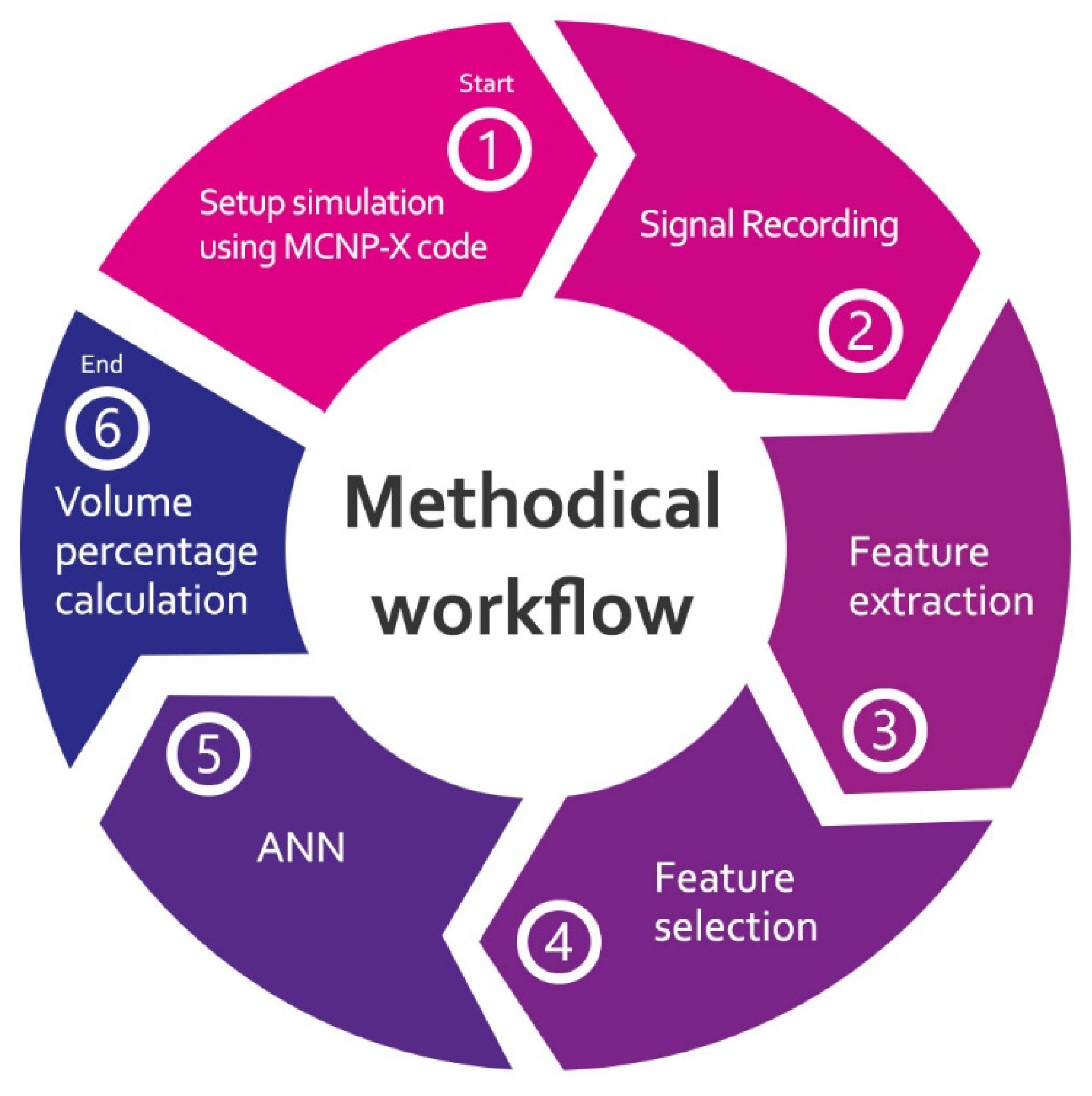
2. Materials and Methods

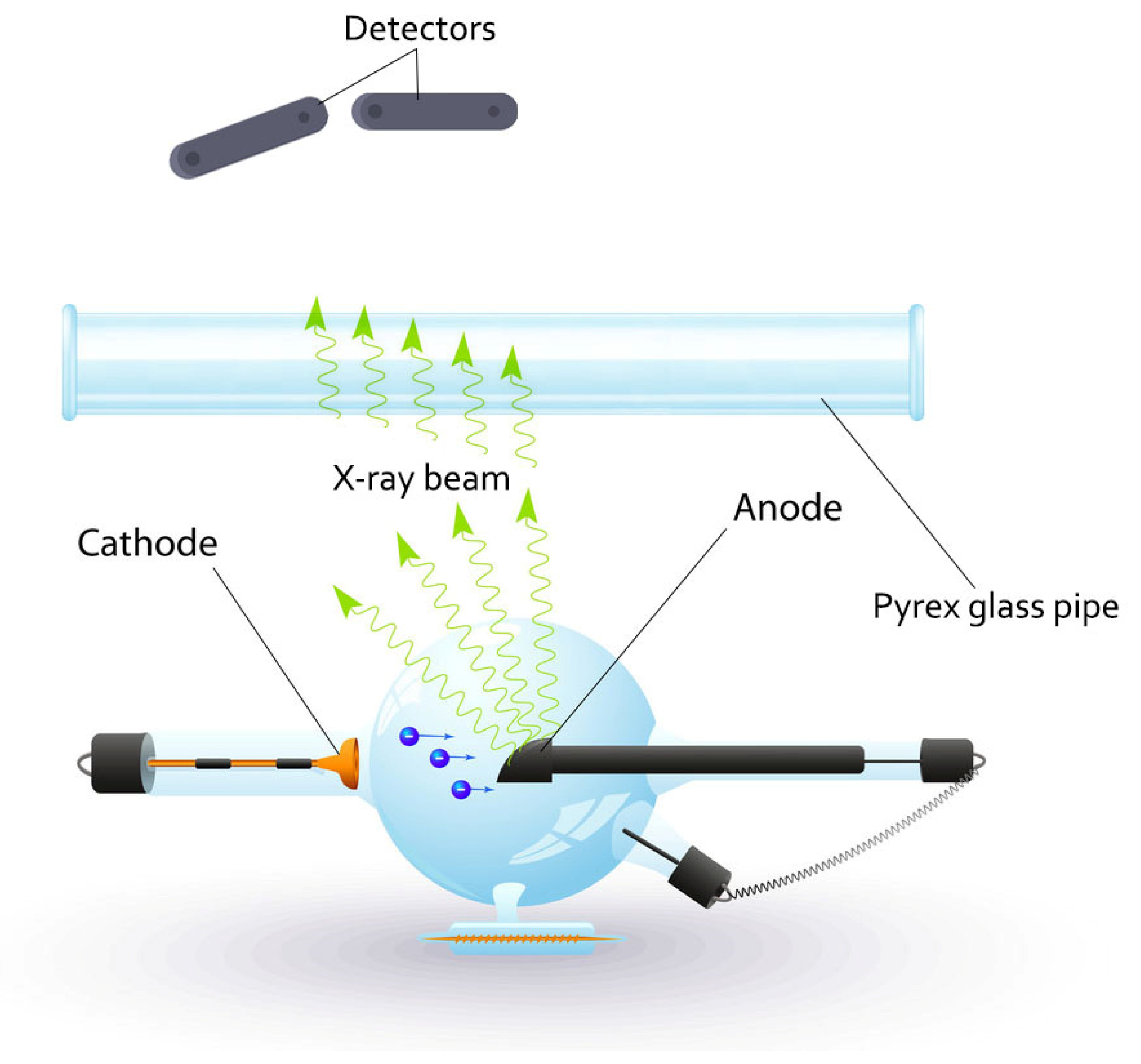
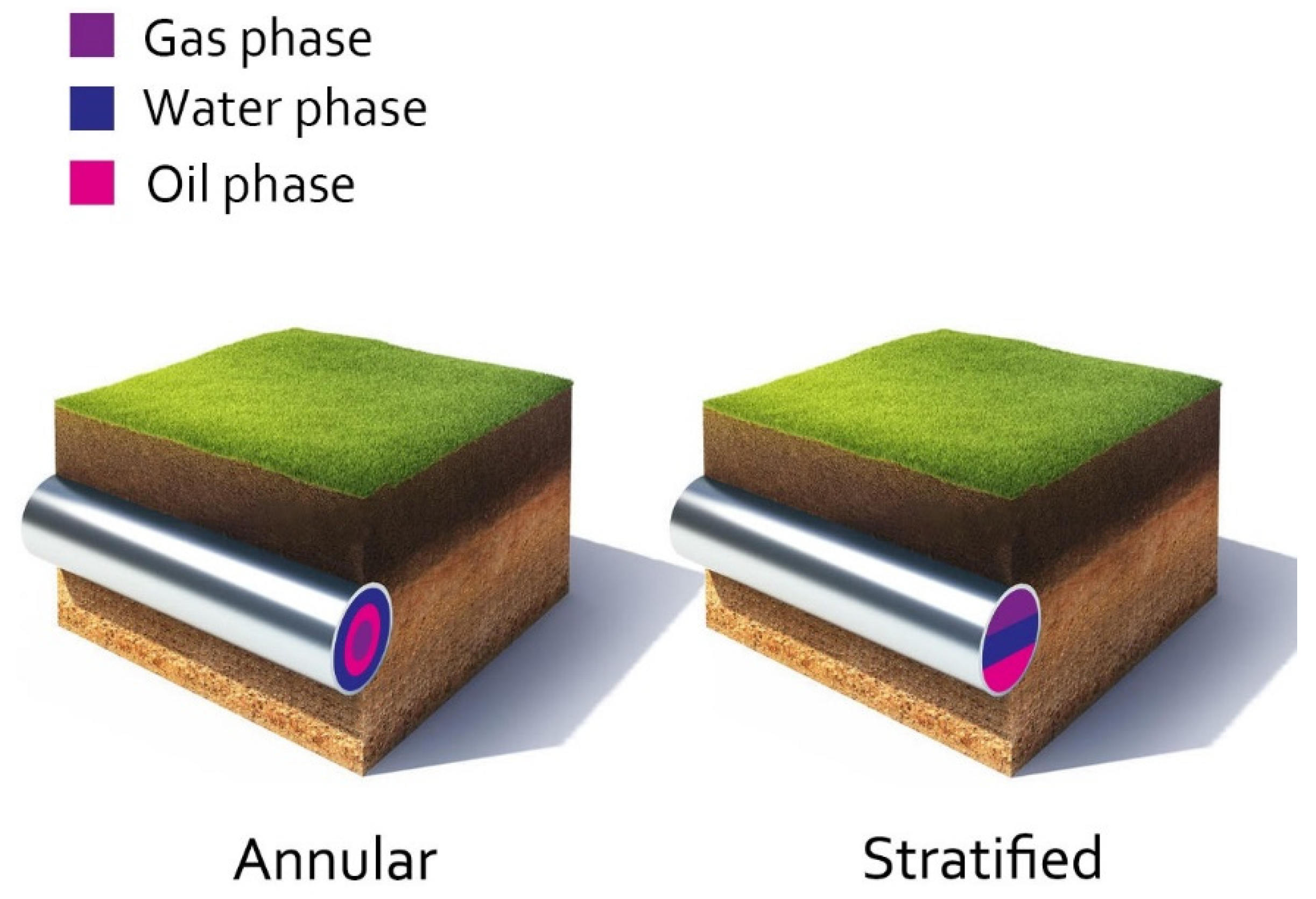
2.1. Radiation-Based System

In this study, the MCNP-X algorithm was used to simulate a detection system made up of an X-ray tube, a Pyrex glass pipe, and two NaI detectors. A pair of detectors, one directly at the source and the other at an angle of 15 degrees from it, were set 20 cm away from the pipe. Different volumes have been simulated in a Pyrex glass. In Figure 2, the basic layout of the proposed system can be seen. From 10 to 80%, with a 10% step, the two most prevalent flow regimes are modeled, as seen in Figure 3. A total of 72 simulations were performed; thirty-six different volume fractions were implemented for each flow pattern. An ordinary X-ray tube was put to work in this investigation. The electron source and the tungsten/rubidium target are housed in X-ray tubes, serving as the cathode and anode, respectively. The complete simulation of an X-ray tube using the MCNPX code is time-consuming since it involves the reaction of an electron emitted from the cathode with the anode, which results in X-ray radiation. This investigation reconsidered a cathode–anode assembly for an X-ray tube with an added photon source due to the lower computational requirements of the MCNPX algorithm for tracking photons than electrons. Hernandez et al.’s open-source software program TASMIC was used in this study [19]. It is worth noting that several studies, both theoretical and MCNP, have been undertaken into the generation of X-ray spectra. Hernandez et al. generated an X-ray spectrum for various tube voltages using the MCNPX program. The input of the MCNPX file was encoded with the obtained X-ray spectrum using the TASMIC package at 150 kV as the tube voltage using the SI and SP selections in the SDEF card to determine the source’s energy. The aforementioned photon source was placed within a cylindrical shielding device for an X-ray tube. The output window is an open area on the shield’s outer layer that allows the X-ray photons that have been created in a favorable environment to emit. For this examination, low-energy photons were blocked by positioning a 2.5 mm thick aluminum filter in front of the X-ray tube’s output window. The recorded X-ray spectra in the detectors are shown in Figure 4.

2.2. Feature Extraction

2.2.1. Frequency Domain

Data reduction, data elimination, training process simplification, and generalization are all possible outcomes of feature extraction, which is conducted on the raw data collected during measurement. Because of this, a better understanding of the data will be formed. In cases when there is an abundance of data but not enough storage space, feature extraction techniques are used to reduce the dimensions while keeping the data’s attributes intact. It is challenging to analyze massive amounts of data, and the created detection system may not work with the data at hand, or it may only work with a subset of the data. Several feature extraction methods exist to minimize the dimensionality of data, such as feature extraction in the time domain, frequency domain, time-frequency domain, wavelet, and even some novel approaches.

For this study, the received signals are converted into the frequency domain using the FTT (Equation (1) [20]) to perform feature extraction in the frequency domain. After that, the signals’ first, second, and third dominating frequencies were extracted.

$$Y\left(k\right)={\displaystyle \sum }_{J=1}^{n}x\left(J\right)w_n^{\left(y-1\right)\left(k-1\right)}$$

(1)

In this case, X is the Fourier transform of Y(k), and $w_n={\mathrm{e}}^{\left(-2\pi \mathrm{i}\right)∕n}$ is one of n roots of unity. Figure 5 displays the frequency domain representations of the received signals for the aforementioned flow regimes.

2.2.2. Wavelet

In order to investigate data with properties that vary with scale, discrete wavelet transforms (DWT) are helpful. Changes in signal frequency, duration, or pattern may be present. The fundamental goal in creating wavelet transforms is to solve problems that the Fourier transform could not provide a solution for it. A wavelet, as opposed to a sine wave, is a fast-decomposing oscillation. The ability to represent data at several scales makes wavelets useful. Various wavelets may be used in various contexts. As stated in [21,22], the DWT is calculated by applying a low-pass filter to the signal with an impulse response of g and then convolving the resulting filters.

$$y\left[n\right]=\left(x\times g\right)\left[n\right]={\sum }_{k=-\infty }^{\infty }x\left[k\right]g\left[n-k\right]$$

(2)

In addition, a second high-pass filter (h) works in tandem to further break down the signal. Figure 6 provides a detailed depiction of a signal’s degeneration. The approach yields both details coefficients (as would be the case with a high-pass filter) and approximations (as would be the case with a low-pass filter). At the conclusion of the filter is a two-stage downsampler. The downsampled output of the low-pass filter provides approximation (a), while the high-pass filter’s low-pass samplers give detail (d). At each successive level, the approximation component may be broken down further into its constituent parts. At this time, the analysis in this research has progressed into the fourth stage. For a given mother wavelet (t), the wavelet operation selects a unique set of child wavelet coefficients. The mother wavelet is scaled and shifted by powers of two in the discrete wavelet transform [21,22]:

$${\psi }_{j,k}=\frac{1}{\sqrt{2^j}}\psi \left(\frac{t-k{2}^j}{2^j}\right)$$

(3)

Scale is indicated by j, and shift by k. The wavelet coefficients obtained from x(t) may be regarded as the projection of x(t) onto a wavelet, given that x(t) represents a 2N-length signal. The following conditions must be met for a member of the aforementioned discrete wavelet family to be considered a child wavelet [21,22]:

$${\gamma }_{jk}={\int }_{-\infty }^{\infty }x\left(t\right)\frac{1}{\sqrt{2^j}}\psi \left(\frac{t-k{2}^j}{2^j}\right)dt$$

(4)

Then, j is a constant, and ${\gamma }_{jk}$ is derived only in terms of a function of k. Sampled at points 1, 2j, 2j,..., 2N, ${\gamma }_{jk}$ is calculated by convolving $x\left(t\right)$ with the mother wavelet signal,$h\left(t\right)=\frac{1}{\sqrt{2^j}}\psi \left(\frac{-t}{2^j}\right)$. Discrete wavelet coefficients at the $j\mathrm{th}$ level are specified here. Therefore, for a given mother wavelet $\psi$(t), a perfect match between the detail coefficients of the filter bank and a wavelet coefficient of a discrete collection of child wavelets is guaranteed by appropriately selecting h[n] and g[n] $\psi$(t). The average a4 and d1–d4 features were calculated from the studied signals and used in the subsequent steps. As already indicated, this research makes use of two detectors, each of which has eight features retrieved from it, including wavelet and frequency domain features, and these characteristics have been used in previous research. However, the big gap in the literature is that no suitable method has been provided to determine the most optimal ones. In this research, we have attempted to introduce the most optimal combination using a PSO-based characteristic selection method [23,24,25,26].

2.3. Feature Selection

Checking out the PSO algorithm is strongly recommended for those studying swarm intelligence [27]. The PSO method has quickly become the gold standard for solving feature selection issues due to its efficiency and ease of use. This approach mimics the communal living habits of fish and birds seen in the environment. The algorithm will need input from everyone in the population to find a solution to the issue. A whole population, indicated by the word “particle,” is uniformly dispersed over the optimized function’s search space. Each particle’s location is evaluated in relation to the objective.

Then, a future direction is chosen by combining knowledge of the current position, the previous ideal location, and the most promising accessible particles. All particle locations will be adjusted before the program continues. This process may be repeated as many as necessary to obtain the desired result. A group of particles striving for the best possible value of a function is analogous to a flock of birds flying around in search of food. The core idea of this method may be expressed as follows: at each given moment, particles relocate to the best accessible place in the search space, taking into account their past observations and the positions of their neighbors. PSO begins with a completely random beginning population, as do other evolutionary algorithms. The first population consists of N randomly selected particles. Vectorial notation is used to describe both particle locations and velocities. Once the value of the cost function has been determined, the particles begin exploring the problem space in quest of a better resting place. Each particle needs a dual-memory system to enable searching. There is just one place to keep track of the best possible present and historical locations for each particle. The particles utilize this data to determine what they should do next. The particles’ velocities and positions are fine-tuned during each iteration to obtain the best possible global and global-average solutions. At each iteration, the particles’ velocities and positions are fine-tuned to achieve the most significant possible absolute and local solutions [28]. Each particle in PSO stands in for a specific answer. Particle I is sought after with the help of two vectors at each iteration: its position, vector X, is $X_i^t$ = [$X_{i1}^t$,$X_{i2}^t$,..., $X_{iD}^t$] and its velocity, vector V, is $V_i^t$ = [$V_{i1}^t$, $V_{i2}^t$,..., $V_{iD}^t$]. The best positions (or solutions) of both the individual particle (denoted by pbesti = [pbesti1, pbesti2,..., pbestiD]) and the population as a whole (denoted by gbest = [gbest1, gbest2,..., gbestD]) are used to update the positions and velocities of the particles as they move. Using the following formulae, the velocity and location of the ith particle are adjusted in accordance with pbest and gbest at the subsequent iteration, t + 1.

$$V_{id}^{t+1}=\omega \times V_{id}^t+c_1\times r_1\times \left(pbes{t}_{id}^t-X_{id}^t\right)+c_2\times r_2\times \left(gbes{t}_d^t-X_{id}^t\right)$$

(5)

$$X_{id}^{t+1}=X_{id}^t+V_{id}^{t+1}$$

(6)

where t and ω stand for the iteration weight and number, respectively, the acceleration constants are c₁ and c₂ (the cognitive and social parameters, respectively), and r₁ and r₂ are evenly distributed and lie between [0, 1]. Defining the cost function is one of the first steps in developing optimization systems. In this research, the mean square error (MSE) of a neural network consisting of one hidden layer and 10 neurons is used as the cost function of the PSO system. The first step involves feeding the network a non-sequential subset of the data’s characteristics. Then, the conventional optimization approach is used to progressively improve the inputs toward ideal values in an effort to minimize the cost function. The PSO system initially tries to foretell the target using a characteristic using an iterative process, then increases the number of inputs as needed and eventually implements the system for all modes with varying inputs.

2.4. MLP Neural Network

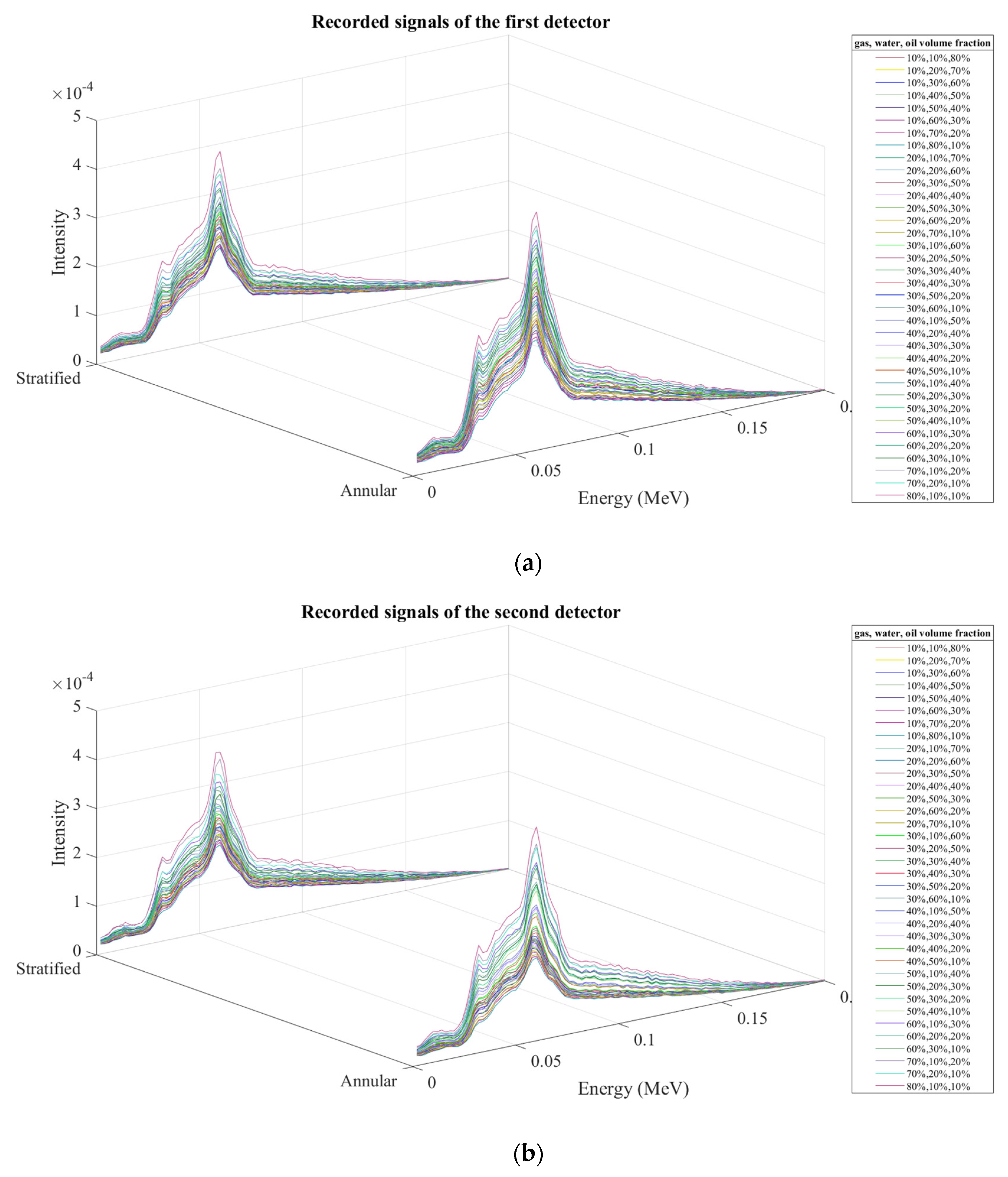
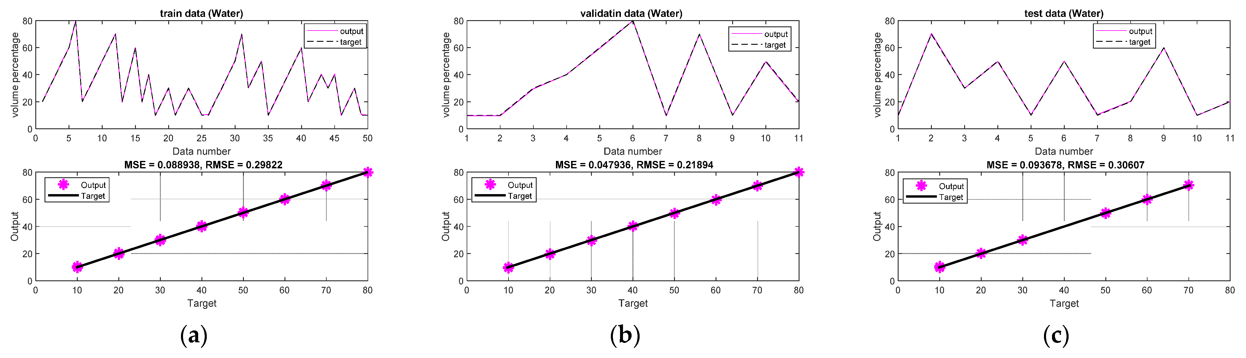
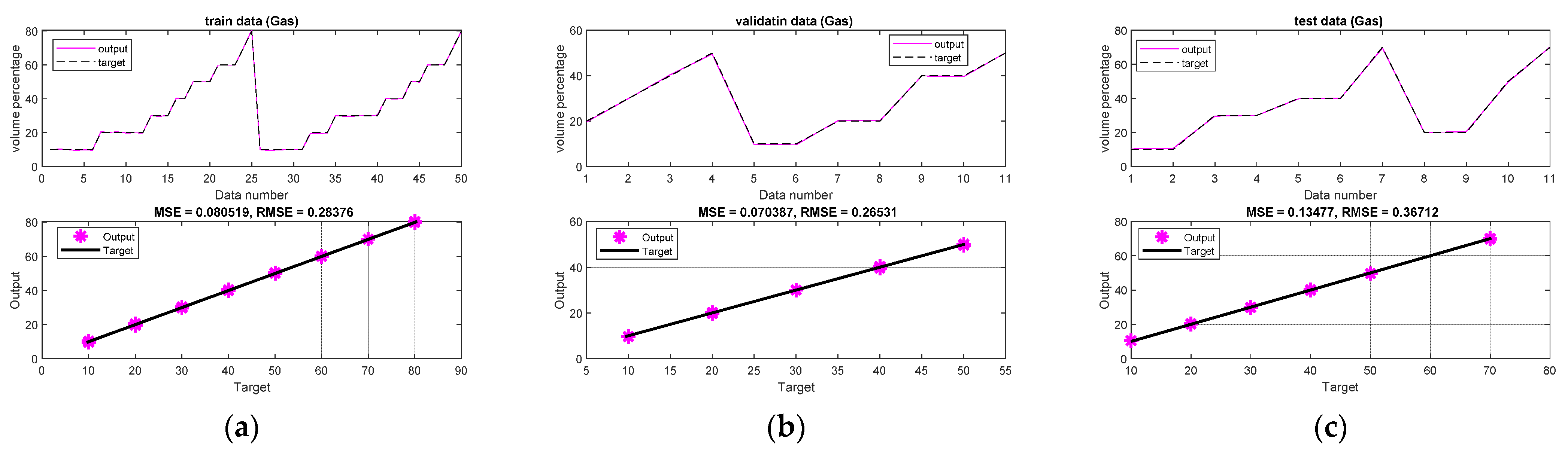
A neuron is a type of computer unit found in the brain; these units include dendrites that serve as an extension for information transmission. When a neuron’s processing steps are complete, the axon will send the data to the rest of the nervous system. Even if the processes indicated occur in the physiological and biochemical realms, the mathematical modeling performed by the researchers has changed the nature of the issue. Many scientists are interested in using artificial neural networks and other mathematically astute scientific techniques in various scientific disciplines [29,30,31,32,33,34,35,36,37,38,39,40,41,42,43,44,45,46,47,48,49,50,51,52,53].

The MLP neural network is one of the most popular models. This network has an input layer, a hidden layer, and an output layer. It is possible for there to be several hidden layers. Mathematical operations, known as activation functions, are carried out in the hidden layers. The nature and degree of non-linearity of the available data determine the number of these layers, the number of neurons in the hidden layer, and the type of activation function. The results of neurons in their mathematical form are as follows [54,55]:

$$n_l={\sum }_{i=1}^u{x}_i{w}_{ij}+b j=1,2,\cdots ,m$$

(7)

$$u_j=f\left({\sum }_{i=1}^u{x}_i{w}_{ij}+b\right) j=1,2,\cdots ,m$$

(8)

$$output={\sum }_{n=1}^j\left(u_n{w}_n\right)+b$$

(9)

where x stands for inputs. Weight “W,” bias “b,” and activation function “f” all stand for different things in this formula. The number of neurons in the hidden layers is denoted by j, where i is the input value. Over- and under-training could be avoided by splitting the available data into training, validation, and testing sets. Most information required to train a neural network consists of examples and patterns. The phrase “validation data” is often used to refer to a subset of the dataset that is utilized to check the efficacy of the training procedure. In order to guarantee a precise performance, the test data are applied to the neural network as a last step in the training process. If a neural network correctly works against the mentioned dataset, it will be robust to operate in actual conditions. In this study, 50 samples were used for training, eleven for validating, and eleven for testing. The research presented here utilized the MATLAB 2018b software to accomplish the tasks of extracting the aforementioned features, implementing i PSO method, and designing the MLP neural network. In MATLAB software, there are many different toolboxes that can be used for training neural networks. However, in the process of designing this network, for more freedom of action, no pre-designed toolboxes were used, and all steps of neural network training were programmed. It is essential to mention that the preset function of newff, which is accessible within MATLAB software, was utilized in order to train the network.

3. Results

The use of the PSO method has many applications in many fields of science [54,55,56,57,58,59]. As mentioned in the previous steps, eight features are extracted from the received signals from two detectors, and 16 are available. These characteristics have been applied to the PSO algorithm to determine the best combination of these characteristics. First, one characteristic is applied as an input to the PSO algorithm to determine how many characteristics are sufficient to determine volume percentages. Then the number of inputs increases in order, and in each case, the PSO algorithm is used to introduce the best combination. Finally, it was found that by choosing seven characteristics out of 16, the value of the cost function reaches the lowest value. Figure 7 clearly shows the value of the cost function in relation to the number of inputs. By examining the best case of selecting seven characteristics out of 16, it was found that the characteristics of Mean{a4}, Mean{d4}, Mean{d2}, Mean{d1} extracted from the first detector and Mean{d4}, Mean{d3}, and Mean{d2} extracted from the second detector were selected as the best combination. As it is known, the frequency characteristics have failed in competition with the wavelet transform characteristics, and only the wavelet transform characteristics have been chosen to determine the volume percentages. These features were defined as the inputs of an MLP neural network. By implementing different MLP neural networks that differed in the number of hidden layers, the number of hidden neurons, and the type of activation function, it was found that a structure with three hidden layers, where the number of neurons in the hidden layers is 20, ten and five was able to predict the volume percentages with very high accuracy. It should be noted that the implemented structure has seven neurons in the input layer and two neurons in the output layer, which was able to predict the volume percentage of gas and water. Additionally, the activation function in the hidden layers was “Tansig”, and in the input and output layers, it was a linear function. The number of epochs in neural network implementation was 450. The designed network structure can be seen in Figure 8.

Mean squared error (MSE) and root-mean-square error (RMSE) were two error measures that were calculated to show the high accuracy of the designed neural network (Equations (10) and (11)). The highest calculated MSE and RMSE in the prediction of volume percentages were equal to 0.13 and 0.36, respectively, which is a very low error value. Fitting and regression diagrams have been used to graphically show the designed neural network’s high accuracy. These diagrams are shown for both network outputs and for all three data sets of training, validation, and testing in Figure 9 and Figure 10. In fitting figures, the output of the neural network is shown with a purple line, and the target output is shown with a black dashed line. In the regression diagram, the stars represent the network’s output, and the line represents the target output. As this figure shows, these two coincide with each other, which shows the high accuracy of the designed neural network. The accuracy of the proposed system is compared to earlier studies in

Table 1. A comparison of the suggested detection system’s precision with earlier research.

Ref	Extracted Features	Feature Selection Method	Type of Neural Network	Maximum MSE	Maximum RMSE
[2]	No feature extraction	Lack of feature selection	MLP	2.56	1.6
[3]	Time features	Lack of feature selection	GMDH	1.24	1.11
[4]	Time features	Lack of feature selection	MLP	0.21	0.46
[9]	Frequency features	Lack of feature selection	MLP	0.67	0.82
[10]	Lack of feature extraction	Lack of feature selection	GMDH	7.34	2.71
[11]	Full energy peak (transmission count), photon counts of Compton edge in the transmission detector, and total count in the scattering detector	Lack of feature selection	MLP	1.08	1.04
[Current study]	Frequency and wavelet features	PSO-based feature selection	MLP	0.13	0.36

. The high accuracy achieved in this research is due to the use of valuable features in neural network training, which is also due to the use of the PSO algorithm as a feature selection system. The extraction of different features, use of different feature selection algorithms, and implementation of different types of neural networks can be discussed and investigated, which requires the special attention of researchers in this field. It is also predicted that the method presented in this research can be effective in improving the performance of many engineering fields [60,61,62].

$$MSE=\frac{{\sum }_{j=1}^N{\left(X_j\left(Exp\right)-X_j\left(Pred\right)\right)}^2}{N}$$

(10)

$$RMSE={\left[\frac{{\sum }_{j=1}^N{\left(X_j\left(Exp\right)-X_j\left(Pred\right)\right)}^2}{N}\right]}^{0.5}$$

(11)

where N is the number of data, “X (Exp)” and “X (Pred)” stands for the experimental and predicted (ANN) values, respectively.

4. Conclusions

Optimizing the system and improving the proficiency of the oil industry can be attained by determining the volume percentage of each condensate phase that passes through the oil pipe. As a result, developing and implementing a system to calculate volume percentages can be helpful in solving the problems of the oil industry. In this research, we sought to investigate the impact of a PSO-based feature selection system on increasing the accuracy of predicting volume fractions. The MCNP code was used to simulate the detection system’s architecture, which included an X-ray tube, a Pyrex glass, and two NaI detectors. Two flow regimes were simulated in different volume percentages, and eight characteristics were extracted from the signals received from each detector, consisting of three frequency characteristics and five wavelet transform characteristics. The extracted characteristics were applied to the PSO algorithm to determine the best combination. Seven characteristics were introduced as the best combination by the PSO algorithm and were considered as the inputs of the MLP neural network. The designed neural network had two outputs that were responsible for determining the volumetric percentage of gas and water. Obviously, the volume percentage of the third phase can be easily calculated by having the volume percentage of the two phases. The maximum MSE value calculated to determine the volume percentages were equal to 0.13. This high accuracy is due to the use of suitable features as neural network inputs selected by the PSO algorithm. In future research, researchers can investigate different characteristics of received signals, using different feature selection methods, and examining different neural networks.

References

1. Salgado, C.M.; Pereira, C.M.; Schirru, R.; Brandão, L.E. Flow regime identification and volume fraction prediction in multiphase flows by means of gamma-ray attenuation and artificial neural networks. Prog. Nucl. Energy 2010, 52, 555–562. [Google Scholar] [CrossRef]
2. Peyvandi, R.G.; Rad, S.Z.I. Application of artificial neural networks for the prediction of volume fraction using spectra of gamma rays backscattered by three-phase flows. Eur. Phys. J. Plus 2017, 132, 511. [Google Scholar] [CrossRef]
3. Sattari, M.A.; Roshani, G.H.; Hanus, R.; Nazemi, E. Applicability of time-domain feature extraction methods and artificial intelligence in two-phase flow meters based on gamma-ray absorption technique. Measurement 2021, 168, 108474. [Google Scholar] [CrossRef]
4. Sattari, M.A.; Roshani, G.H.; Hanus, R. Improving the structure of two-phase flow meter using feature extraction and GMDH neural network. Radiat. Phys. Chem. 2020, 171, 108725. [Google Scholar] [CrossRef]
5. Roshani, G.; Nazemi, E.; Roshani, M. Intelligent recognition of gas-oil-water three-phase flow regime and determination of volume fraction using radial basis function. Flow Meas. Instrum. 2017, 54, 39–45. [Google Scholar] [CrossRef]
6. Hanus, R.; Zych, M.; Petryka, L.; Jaszczur, M.; Hanus, P. Signals features extraction in liquid-gas flow measurements using gamma densitometry. Part 1: Time domain. EPJ Web Conf. 2016, 114, 02035. [Google Scholar] [CrossRef] [Green Version]
7. Hanus, R.; Zych, M.; Petryka, L.; Jaszczur, M.; Hanus, P. Signals features extraction in liquid-gas flow measurements using gamma densitometry. Part 2: Frequency domain. EPJ Web Conf. 2016, 114, 02036. [Google Scholar] [CrossRef] [Green Version]
8. Hanus, R.; Zych, M.; Kusy, M.; Jaszczur, M.; Petryka, L. Identification of liquid-gas flow regime in a pipeline using gamma-ray absorption technique and computational intelligence methods. Flow Meas. Instrum. 2018, 60, 17–23. [Google Scholar] [CrossRef]
9. Hosseini, S.; Roshani, G.; Setayeshi, S. Precise gamma based two-phase flow meter using frequency feature extraction and only one detector. Flow Meas. Instrum. 2020, 72, 101693. [Google Scholar] [CrossRef]
10. Roshani, M.; Sattari, M.A.; Ali, P.J.M.; Roshani, G.H.; Nazemi, B.; Corniani, E.; Nazemi, E. Application of GMDH neural network technique to improve measuring precision of a simplified photon attenuation based two-phase flowmeter. Flow Meas. Instrum. 2020, 75, 101804. [Google Scholar] [CrossRef]
11. Roshani, G.H.; Nazemi, E.; Feghhi, S.A.; Setayeshi, S. Flow regime identification and void fraction prediction in two-phase flows based on gamma ray attenuation. Measurment 2015, 62, 25–32. [Google Scholar] [CrossRef]
12. Nazemi, E.; Roshani, G.H.; Feghhi, S.A.H.; Setayeshi, S.; Zadeh, E.E.; Fatehi, A. Optimization of a method for identifying the flow regime and measuring void fraction in a broad beam gamma-ray attenuation technique. Int. J. Hydrog. Energy 2016, 41, 7438–7444. [Google Scholar] [CrossRef]
13. Roshani, G.H.; Nazemi, E.; Roshani, M.M. Flow regime independent volume fraction estimation in three-phase flows using dual-energy broad beam technique and artificial neural network. Neural Comput. Appl. 2016, 28, 1265–1274. [Google Scholar] [CrossRef]
14. Nazemi, E.; Feghhi, S.A.H.; Roshani, G.H.; Peyvandi, R.G.; Setayeshi, S. Precise Void Fraction Measurement in Two-phase Flows Independent of the Flow Regime Using Gamma-ray Attenuation. Nucl. Eng. Technol. 2016, 48, 64–71. [Google Scholar] [CrossRef] [Green Version]
15. Song, K.; Liu, Y. A compact X-ray system for two-phase flow measurement. Meas. Sci. Technol. 2017, 29, 025305. [Google Scholar] [CrossRef]
16. Roshani, M.; Ali, P.J.M.; Roshani, G.H.; Nazemi, B.; Corniani, E.; Phan, N.H.; Tran, H.N.; Nazemi, E. X-ray tube with artificial neural network model as a promising alternative for radioisotope source in radiation based two phase flowmeters. Appl. Radiat. Isot. 2020, 164, 109255. [Google Scholar] [CrossRef]
17. Roshani, M.; Phan, G.; Roshani, G.H.; Hanus, R.; Nazemi, B.; Corniani, E.; Nazemi, E. Combination of X-ray tube and GMDH neural network as a nondestructive and potential technique for measuring characteristics of gas-oil–water three phase flows. Measurement 2021, 168, 108427. [Google Scholar] [CrossRef]
18. Roshani, G.H.; Ali, P.J.M.; Mohammed, S.; Hanus, R.; Abdulkareem, L.; Alanezi, A.A.; Nazemi, E.; Eftekhari-Zadeh, E.; Kalmoun, E.M. Feasibility Study of Using X-ray Tube and GMDH for Measuring Volume Fractions of Annular and Stratified Regimes in Three-Phase Flows. Symmetry 2021, 13, 613. [Google Scholar] [CrossRef]
19. Hernandez, A.M.; Boone, J.M. Tungsten anode spectral model using interpolating cubic splines: Unfiltered x-ray spectra from 20 kV to 640 kV. Med. Phys. 2014, 41, 042101. [Google Scholar] [CrossRef] [Green Version]
20. Nussbaumer, H.J. The fast Fourier transforms. In Fast Fourier Transform and Convolution Algorithms; Springer: Berlin/Heidelberg, Germany, 1981; pp. 80–111. [Google Scholar]
21. Daubechies, I. The wavelet transform, time-frequency localization and signal analysis. IEEE Trans. Inf. Theory 1990, 36, 961–1005. [Google Scholar] [CrossRef]
22. Soltani, S. On the use of the wavelet decomposition for time series prediction. Neurocomputing 2002, 48, 267–277. [Google Scholar] [CrossRef]
23. Taylan, O.; Sattari, M.A.; Essoussi, I.E.; Nazemi, E. Frequency Domain Feature Extraction Investigation to Increase the Accuracy of an Intelligent Nondestructive System for Volume Fraction and Regime Determination of Gas-Water-Oil Three-Phase Flows. Mathematics 2021, 9, 2091. [Google Scholar] [CrossRef]
24. Balubaid, M.; Sattari, M.A.; Taylan, O.; Bakhsh, A.A.; Nazemi, E. Applications of Discrete Wavelet Transform for Feature Extraction to Increase the Accuracy of Monitoring Systems of Liquid Petroleum Products. Mathematics 2021, 9, 3215. [Google Scholar] [CrossRef]
25. Iliyasu, A.M.; Mayet, A.M.; Hanus, R.; El-Latif, A.A.A.; Salama, A.S. Employing GMDH-Type Neural Network and Signal Frequency Feature Extraction Approaches for Detection of Scale Thickness inside Oil Pipelines. Energies 2022, 15, 4500. [Google Scholar] [CrossRef]
26. Mayet, A.M.; Alizadeh, S.M.; Hamakarim, K.M.; Al-Qahtani, A.A.; Alanazi, A.K.; Guerrero, J.W.G.; Alhashim, H.H.; Eftekhari-Zadeh, E. Application of Wavelet Characteristics and GMDH Neural Networks for Precise Estimation of Oil Product Types and Volume Fractions. Symmetry 2022, 14, 1797. [Google Scholar] [CrossRef]
27. Kennedy, J.; Eberhart, R. Particle Swarm Optimization. In Proceedings of the ICNN’95—International Conference on Neural Networks, Perth, Australia, 27 November–1 December 1995; Volume 4, pp. 1942–1948. [Google Scholar] [CrossRef]
28. Shi, Y.; Eberhart, R. A modified particle swarm optimizer. In Proceedings of the 1998 IEEE International Conference on Evolutionary Computation Proceedings. IEEE World Congress on Computational Intelligence (Cat. No. 98TH8360), Anchorage, AK, USA, 4–9 May 1998; pp. 69–73. [Google Scholar] [CrossRef]
29. Sattari, M.A.; Korani, N.; Hanus, R.; Roshani, G.H.; Nazemi, E. Improving the performance of gamma radiation based two phase flow meters using optimal time characteristics of the detector output signal extraction. J. Nucl. Sci. Technol. (JonSat) 2020, 41, 42–54. [Google Scholar]
30. Khaibullina, K. Technology to remove asphaltene, resin and paraffin deposits in wells using organic solvents. In Proceedings of the SPE Annual Technical Conference and Exhibition 2016, Dubai, United Arab Emirates, 26–28 September 2016. [Google Scholar]
31. Tikhomirova, E.A.; Sagirova, L.R.; Khaibullina, K.S. A review on methods of oil saturation modelling using IRAP RMS. IOP Conf. Series Earth Environ. Sci. 2019, 378, 012075. [Google Scholar] [CrossRef]
32. Khaibullina, K.S.; Korobov, G.Y.; Lekomtsev, A.V. Development of an asphalt-resin-paraffin deposits inhibitor and substantiation of the technological parameters of its injection into the bottom-hole formation zone. Period. Tche Quim. 2020, 17, 769–781. [Google Scholar] [CrossRef]
33. Khaibullina, K.S.; Sagirova, L.R.; Sandyga, M.S. Substantiation and selection of an inhibitor for preventing the formation of asphalt-resin-paraffin deposits. Period. Tche Quim. 2020, 17, 541–551. [Google Scholar] [CrossRef]
34. Mayet, A.M.; Alizadeh, S.M.; Kakarash, Z.A.; Al-Qahtani, A.A.; Alanazi, A.K.; Alhashimi, H.H.; Eftekhari-Zadeh, E.; Nazemi, E. Introducing a Precise System for Determining Volume Percentages Independent of Scale Thickness and Type of Flow Regime. Mathematics 2022, 10, 1770. [Google Scholar] [CrossRef]
35. Mayet, A.M.; Alizadeh, S.M.; Nurgalieva, K.S.; Hanus, R.; Nazemi, E.; Narozhnyy, I.M. Extraction of Time-Domain Characteristics and Selection of Effective Features Using Correlation Analysis to Increase the Accuracy of Petroleum Fluid Monitoring Systems. Energies 2022, 15, 1986. [Google Scholar] [CrossRef]
36. Lalbakhsh, A.; Mohamadpour, G.; Roshani, S.; Ami, M.; Roshani, S.; Sayem, A.S.M.; Alibakhshikenari, M.; Koziel, S. Design of a Compact Planar Transmission Line for Miniaturized Rat-Race Coupler with Harmonics Suppression. IEEE Access 2021, 9, 129207–129217. [Google Scholar] [CrossRef]
37. Hookari, M.; Roshani, S.; Roshani, S. High-efficiency balanced power amplifier using miniaturized harmonics suppressed coupler. Int. J. RF Microw. Comput. Aided Eng. 2020, 30, e22252. [Google Scholar] [CrossRef]
38. Lotfi, S.; Roshani, S.; Roshani, S.; Gilan, M.S. Wilkinson power divider with band-pass filtering response and harmonics suppression using open and short stubs. Frequenz 2020, 74, 169–176. [Google Scholar] [CrossRef]
39. Jamshidi, M.; Siahkamari, H.; Roshani, S.; Roshani, S. A compact Gysel power divider design using U-shaped and T-shaped resonators with harmonics suppression. Electromagnetics 2019, 39, 491–504. [Google Scholar] [CrossRef]
40. Roshani, S.; Jamshidi, M.B.; Mohebi, F.; Roshani, S. Design and modeling of a compact power divider with squared resonators using artificial intelligence. Wirel. Pers. Commun. 2021, 117, 2085–2096. [Google Scholar] [CrossRef]
41. Roshani, S.; Azizian, J.; Roshani, S.; Jamshidi, M.; Parandin, F. Design of a miniaturized branch line microstrip coupler with a simple structure using artificial neural network. Frequenz 2022, 76, 255–263. [Google Scholar] [CrossRef]
42. Khaleghi, M.; Salimi, J.; Farhangi, V.; Moradi, M.J.; Karakouzian, M. Application of Artificial Neural Network to Predict Load Bearing Capacity and Stiffness of Perforated Masonry Walls. Civileng 2021, 2, 48–67. [Google Scholar] [CrossRef]
43. Zych, M.; Petryka, L.; Kępński, J.; Hanus, R.; Bujak, T.; Puskarczyk, E. Radioisotope investigations of compound two-phase flows in an ope channel. Flow Meas. Instrum. 2014, 35, 11–15. [Google Scholar] [CrossRef]
44. Zych, M.; Hanus, R.; Wilk, B.; Petryka, L.; Świsulski, D. Comparison of noise reduction methods in radiometric correlation measurements of two-phase liquid-gas flows. Measurement 2018, 129, 288–295. [Google Scholar] [CrossRef]
45. Golijanek-Jędrzejczyk, A.; Mrowiec, A.; Hanus, R.; Zych, M.; Heronimczak, M.; Świsulski, D. Uncertainty of mass flow measurement using centric and eccentric orifice for Reynolds number in the range 10,000 ≤ Re ≤ 20,000. Measurement 2020, 160, 107851. [Google Scholar] [CrossRef]
46. Mayet, A.; Hussain, M. Amorphous WNx Metal For Accelerometers and Gyroscope. In Proceedings of the MRS Fall Meeting, Boston, MA, USA, 30 November–5 December 2014. [Google Scholar]
47. Mayet, A.M.; Hussain, A.M.; Hussain, M.M. Three-terminal nanoelectromechanical switch based on tungsten nitride—An amorphous metallic material. Nanotechnology 2015, 27, 035202. [Google Scholar] [CrossRef] [PubMed]
48. Shukla, N.K.; Mayet, A.M.; Vats, A.; Aggarwal, M.; Raja, R.K.; Verma, R.; Muqeet, M.A. High speed integrated RF–VLC data communication system: Performance constraints and capacity considerations. Phys. Commun. 2021, 50, 101492. [Google Scholar] [CrossRef]
49. Dabiri, H.; Farhangi, V.; Moradi, M.J.; Zadehmohamad, M.; Karakouzian, M. Applications of Decision Tree and Random Forest as Tree-Based Machine Learning Techniques for Analyzing the Ultimate Strain of Spliced and Non-Spliced Reinforcement Bars. Appl. Sci. 2022, 12, 4851. [Google Scholar] [CrossRef]
50. Mayet, A.; Smith, C.E.; Hussain, M.M. Energy reversible switching from amorphous metal based nanoelectromechanical switch. In Proceedings of the 13th IEEE International Conference on Nanotechnology (IEEE-NANO 2013), Beijing, China, 5–8 August 2013; pp. 366–369. [Google Scholar]
51. Alamoudi, M.; Sattari, M.; Balubaid, M.; Eftekhari-Zadeh, E.; Nazemi, E.; Taylan, O.; Kalmoun, E. Application of Gamma Attenuation Technique and Artificial Intelligence to Detect Scale Thickness in Pipelines in Which Two-Phase Flows with Different Flow Regimes and Void Fractions Exist. Symmetry 2021, 13, 1198. [Google Scholar] [CrossRef]
52. Karami, A.; Roshani, G.H.; Khazaei, A.; Nazemi, E.; Fallahi, M. Investigation of different sources in order to optimize the nuclear metering system of gas–oil–water annular flows. Neural Comput. Appl. 2020, 32, 3619–3631. [Google Scholar] [CrossRef]
53. Roshani, G.H.; Ali, P.J.M.; Mohammed, S.; Hanus, R.; Abdulkareem, L.; Alanezi, A.A.; Sattari, M.A.; Amiri, S.; Nazemi, E.; Eftekhari-Zadeh, E.; et al. Simulation Study of Utilizing X-ray Tube in Monitoring Systems of Liquid Petroleum Products. Processes 2021, 9, 828. [Google Scholar] [CrossRef]
54. Taylor, J.G. Neural Networks and Their Applications; John Wiley & Sons Ltd.: Brighton, UK, 1996. [Google Scholar]
55. Gallant, A.R.; White, H. On learning the derivatives of an unknown mapping with multilayer feedforward networks. Neural Netw. 1992, 5, 129–138. [Google Scholar] [CrossRef] [Green Version]
56. Abunadi, I.; Albraikan, A.A.; Alzahrani, J.S.; Eltahir, M.M.; Hilal, A.M.; Eldesouki, M.I.; Motwakel, A.; Yaseen, I. An Automated Glowworm Swarm Optimization with an Inception-Based Deep Convolutional Neural Network for COVID-19 Diagnosis and Classification. Healthcare 2022, 10, 697. [Google Scholar] [CrossRef]
57. Ahmad, M.; Khaja, I.A.; Baz, A.; Alhakami, H.; Alhakami, W. Particle Swarm Optimization Based Highly Nonlinear Substitution-Boxes Generation for Security Applications. IEEE Access 2020, 8, 116132–116147. [Google Scholar] [CrossRef]
58. Alshareef, M.; Lin, Z.; Ma, M.; Cao, W. Accelerated Particle Swarm Optimization for Photovoltaic Maximum Power Point Tracking under Partial Shading Conditions. Energies 2019, 12, 623. [Google Scholar] [CrossRef] [Green Version]
59. Alshareef, M. A New Particle Swarm Optimization with Bat Algorithm Parameter-Based MPPT for Photovoltaic Systems under Partial Shading Conditions. Stud. Inform. Control. 2022, 31, 53–66. [Google Scholar] [CrossRef]
60. Khalaj, O.; Jamshidi, M.B.; Saebnoori, E.; Masek, B.; Stadler, C.; Svoboda, J. Hybrid Machine Learning Techniques and Computational Mechanics: Estimating the Dynamic Behavior of Oxide Precipitation Hardened Steel. IEEE Access 2021, 9, 156930–156946. [Google Scholar] [CrossRef]
61. Jamshidi, M.B.; Roshani, S.; Talla, J.; Roshani, S. Using an ANN approach to estimate output power and PAE of a modified class-F power amplifier. In Proceedings of the 2020 International Conference on Applied Electronics (AE), Pilsen, Czech Republic, 8–9 September 2020; pp. 1–6. [Google Scholar]
62. Jamshidi, M.; Siahkamari, H.; Jamshidi, M. Using artificial neural networks and system identification methods for electricity price modeling. In Proceedings of the 2017 3rd Iranian Conference on Intelligent Systems and Signal Processing (ICSPIS), Shahrood, Iran, 20–21 December 2017; pp. 43–47. [Google Scholar]
Figure 1. Methodical workflow of the proposed manner.
Processes 11 00236 g001
Figure 2. Proposed detection system structure.
Processes 11 00236 g002
Figure 3. Simulated flow regimes.
Processes 11 00236 g003
Figure 4. The signals recorded by the (a) first and (b) second detectors correspond to simulated flow regimes in different volume percentages.
Processes 11 00236 g004
Figure 5. Transmitted signals to the frequency domain of (a) the first detector and (b) the second detector.
Processes 11 00236 g005
Figure 6. Detail and approximation signals extracted by wavelet transform.
Processes 11 00236 g006
Figure 7. The value of the cost function is calculated by the PSO algorithm in terms of the number of features.
Processes 11 00236 g007
Figure 8. The implemented neural network structure to determine the volumetric percentages of gas and water.
Processes 11 00236 g008
Figure 9. Regression diagram related to the prediction of water volume percentage for (a) training, (b) validation, and (c) test data.
Processes 11 00236 g009
Figure 10. Regression diagram related to the prediction of gas volume percentage for (a) training, (b) validation, and (c) test data.
Processes 11 00236 g010