Prediction Method of Tunnel Natural Wind Based on Open-Source Meteorological Parameters

Abstract

The rational use of natural wind in extra-long tunnels for feedforward operation ventilation control can dramatically reduce tunnel operation costs. However, traditional tunnel natural wind calculation theory lacks a prediction function. This paper proposes a three-stage tunnel natural wind prediction method relying on the Yanglin Tunnel in Yunnan, China based on the massive meteorological parameters provided by the open-source national meteorological stations around the tunnel, which make up for the partial deficiency of the meteorological parameters of the tunnel portal. The multi-layer perceptron model (MLP) was used to predict the real-time meteorological parameters of the tunnel portal using the data from four national meteorological stations. The nonlinear autoregressive network model (NARX) was used to predict the meteorological parameters of the tunnel portal in the next period based on the predicted and measured real-time data. The natural wind speed in the tunnel was obtained by a theoretical calculation method using the predicted meteorological parameters. The final tunnel natural wind prediction results are in good agreement with the field measured data, which indicates that the research results of this paper can play a guiding role in the feedforward regulation of tunnel operation fans.

1. Introduction

With the vigorous construction of China’s national expressway network, the number and length of highway tunnels are increasing rapidly. By the end of 2020, China had built 1394 extra-long tunnels with a length of 6235.5 km and 5541 long tunnels with a total length of 9632.2 km [1]. The increase in the number of long highway tunnels is accompanied by a significant increase in tunnel ventilation accessory structures and facilities, and the operation ventilation cost of highway tunnels can reach up to 70% of the total operation cost [2]. Typical ventilation schemes of some extra-long highway tunnels in China are shown in

Table 1. Ventilation schemes of extra-long highway tunnels in China.

Tunnel	Tunnel Length/(km)	Ventilation Scheme	Ventilation Section
Qinling Zhongnanshan Tunnel	18.0	Feed and exhaust longitudinal ventilation with air supply through parallel heading	4
Jinpingshan Tunnel	17.5	Longitudinal jet ventilation	1
Qinling Tiantaishan Tunnel	15.6	Feed and exhaust longitudinal ventilation	4
Erlangshan Tunnel	13.4	Feed and exhaust longitudinal ventilation	3
Shiziping Tunnel	13.1	Feed and exhaust longitudinal ventilation	3 in right line, 2 in left line
Maijishan Tunnel	12.3	Feed and exhaust longitudinal ventilation	4 in right line, 3 in left line

.

Existing designs often consider tunnel natural wind as ventilation resistance [3]. In some cold areas, the natural wind will lead to a longer tunnel freezing length [4], and it is necessary to prevent cold natural wind from entering the tunnel [5]. However, as an important factor affecting the economy and safety of tunnel ventilation design, natural wind utilization technology is one of the main optimization directions of highway tunnel operation ventilation at present. Previous studies have shown that indoor air quality can be improved with the rational use of natural wind [6,7]. Moreover, the size and characteristics of the tunnel natural wind can be obtained by theoretical calculations, model tests, and numerical simulations [8,9,10]. In addition, since extra-long tunnels often cross the climate isolation zone, the influence of the tunnel natural wind on ventilation is more obvious than that in other areas [11]. The tunnel operation cost can be greatly reduced if the tunnel natural wind is fully and reasonably used [12]. For example, Mao et al. (2012) have drawn the conclusion that the natural ventilation can reduce the total operation investment of a city tunnel by 30% [13]. Due to the huge utilization potential of tunnel natural wind, how to use it accurately and scientifically has become a major research trend.

The size and characteristics of the tunnel natural wind will change with the change in the natural environmental conditions outside the tunnel [14]. The accurate prediction of the tunnel natural wind speed in the next period can guide the regulation of the fan in time and achieve further energy saving. For the time being, the research on wind speed prediction is more concentrated in the field of wind power generation [15]. In retrospect, multiple forecasting models are adopted to predict wind speed. Li et al. (2010) conducted a comprehensive comparative study on the accuracy degree of the wind speed prediction of three typical neural networks: adaptive linear element, back propagation, and radial basis function. It is concluded that no neural network model is superior to other models in all evaluation indexes [16]. Zhao et al. (2012) used a coupled model consisting of a Numerical Weather Prediction (NWP) model and Artificial Neural Networks (ANNs) to improve the accuracy of wind speed prediction [17]. Shi et al. (2014) used a hybrid prediction model based on grey correlation analysis and wind speed distribution characteristics to predict very short-term wind power output [18]. Bastos et al. (2021) developed an improved U-convolutional model for spatio-temporal wind speed prediction [19]. Sacie et al. (2022) found that the NARX model performed best in terms of metocean variables prediction among several machine learning models [20].

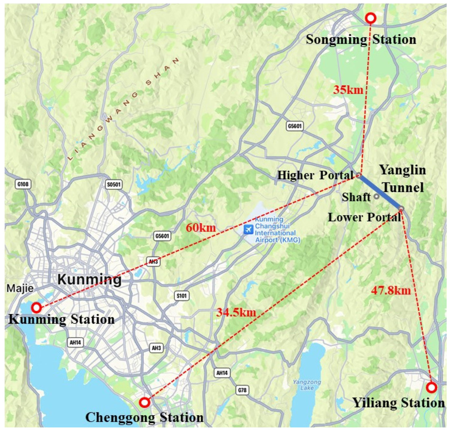
In summary, the calculation of natural wind in highway tunnels mostly depends on theoretical calculations, model tests, and numerical simulations, while the prediction of meteorological parameters in a complex terrain is often concentrated in the field of wind power generation. In order to use the tunnel natural wind achieving feed-forward operation ventilation, it is necessary to conduct deeper research by combining the meteorological parameter prediction method and the tunnel natural wind calculation theory. In this study, a predictive learning model of deep multi-tasking is established based on the Yanglin Tunnel project, which contains data from multiple spatio-temporal-related sites for training at the same time. The purpose is to predict the natural wind of mountain tunnels as accurately as possible based on the open-source data of the national meteorological station and provide a reference for the feedforward operation ventilation regulation of highway tunnels.

2. Prediction and Calculation Method

2.1. Research Frame

The existing natural wind calculation theory is based on the meteorological parameters of the tunnel portals. In order to achieve the purpose of feed-forward energy-saving ventilation in the tunnel, it is necessary to establish a set of natural wind prediction methods. Meteorological stations are installed at the lower portal, higher portal, and shaft of Yanglin Tunnel. However, due to the short construction and operation time of Yanglin Tunnel, the establishment time of meteorological stations lags the tunnel operation time, and the meteorological stations will face the risk of being damaged or dismantled in the future, resulting in a small number of samples of meteorological data at the tunnel portal at any moment, which cannot achieve effective prediction. Fortunately, there are four open-source ground observation stations of the China Meteorological Administration around the tunnel, with sufficient data samples which are easy to obtain. Among them, Songming Station and Kunming Station are in the north and southwest of the higher portal, about 35 km and 60 km away, respectively. Chenggong Station and Yiliang Station are in the south and southwest of the lower portal, about 34.5 km and 47.8 km away, respectively. The geographical relationship between the four national meteorological stations and the meteorological stations around the tunnel is shown in Figure 1.

In this paper, a three-stage prediction method of tunnel natural wind based on the open-source data of the national meteorological station is developed. The first stage is to obtain the real-time meteorological data of the tunnel portal according to the open-source data of the national meteorological station; the second stage is to predict the meteorological data of the next period according to the predicted and measured real-time meteorological data of the tunnel portal; the third stage is to calculate the tunnel natural wind according to the predicted meteorological data of the tunnel portal in the next period. The required meteorological parameters are wind speed, wind direction, temperature, barometric pressure, and relative humidity. The whole prediction processes of the tunnel natural wind are shown in Figure 2.

2.2. Real-Time Data Acquisition Method

In order to support the prediction of meteorological parameters by using the data of the national meteorological station, it is necessary to determine the transmission relationship between each parameter and the meteorological stations. In this paper, multi-layer perceptron (MLP) is used to analyze the spatio-temporal characteristics of each piece of data to obtain the real-time meteorological parameters of the tunnel portal. MLP is a standard fully connected neural network model composed of multiple node layers, which is usually used to explore modeling, binary classification, multi-classification, and regression problems [21]. In this section, a multi-layer perceptron network containing three dense layers is established to realize the regression analysis of meteorological data at the tunnel portal. The prediction structure of the multi-layer perceptron is shown in Figure 3.

2.2.1. Data Collection and Input

The required meteorological parameters are wind speed, wind direction, temperature, barometric pressure, and relative humidity. The prediction of a certain meteorological parameter of each station is taken as a task, one station is defined as the main task, and three neighboring stations are selected as auxiliary tasks. The influencing factors of several meteorological parameters were constructed into a two-dimensional matrix, and each input sample was composed of four surrounding national meteorological stations and three stations at the tunnel portal of the Yanglin Tunnel. Each sampling point contains hourly sampling data with uniform parameters.

2.2.2. Spatio-Temporal Correlation Analysis

After the data input, the flow of data is shown in Figure 4.

The features extracted from multiple tasks are simultaneously transferred to the shared layer composed of multi-layer neural networks. Multiple tasks share parameters in the shared layer to learn the spatio-temporal correlation characteristics of multiple sites. Finally, the correlation matrix is used to represent the correlation between input variables and output variables, and the calculation dimension is reduced by eliminating highly correlated variables. The correlation matrix of the wind speed of each weather station is shown in

Table 2. Wind speed correlation analysis of each weather station.

Correlation	L.P.	H.P.	Shaft	Kun.	Song.	Yi.	Cheng.
L.P.(1)	1	0.48	0.85	0.76	0.95	0	0.21
H.P.(2)	0.48	1	0.28	0.3	0.81	0.92	0.9
Shaft	0.85	0.28	1	0.71	0.78	0.02	0.87
Kun.(3)	0.76	0.3	0.71	1	0.8	0.17	0.91
Song.(4)	0.95	0.81	0.78	0.8	1	0.94	0.76
Yi.(5)	0	0.92	0.02	0.17	0.94	1	0.06
Cheng.(6)	0.21	0.9	0.87	0.76	0.76	0.06	1

⁽¹⁾ L.P.: lower portal. ⁽²⁾ H.P.: higher portal. ⁽³⁾ Kun.: Kunming station. ⁽⁴⁾ Song.: Songming station. ⁽⁵⁾ Yi.: Yiliang station. ⁽⁶⁾ Cheng.: Chenggong station.

. The others are similar and will not be repeated.

2.2.3. Machine Learning with Heterogeneous Features

As shown in Figure 4, multiple tasks enter their own unique fully connected deep neural network, and each task uses its own MLP to learn its time series features and mines personalized information. Each task calculates the loss value according to the predicted value and the observed value and obtains the different losses of multiple tasks. Then, the multiple loss values are jointly optimized by weighted summation so that each task can better consider the results of their mutual influence in the learning process. In this process, the stochastic gradient descent algorithm is used for continuous iterative training to minimize the objective function. When the error of the verification set is no longer reduced, use the early stopping function to stop the training, and save the parameter decreasing to the lowest as the final model.

The final prediction model expressions of each tunnel portal are obtained as follows:

$$f\left(x\right)={\displaystyle \sum }_{i=1}^n\left|{\alpha }_i-{\alpha }_n\right|K\left(x_i,x\right)+o\left(x\right)$$

(1)

where ${\alpha }_i$ is the weight value of the input points of each weather station, as shown in

Table 3. Meteorological parameter prediction weight value.

Parameter	Location	Kun.	Song.	Yi.	Cheng.
W.S.(1)	Lower portal	0.974	0.967	1.095	0.867
W.D.(2)		0.845	0.857	1.054	1.002
Temperature		0.996	0.987	0.896	0.876
B.P.(3)		0.786	0.798	0.973	0.837
R.H.(4)		0.876	0.895	0.967	0.892
W.S.	Higher portal	1.020	1.013	1.096	0.896
W.D.		0.878	0.800	1.098	1.053
Temperature		1.040	0.971	0.859	0.928
B.P.		0.815	0.761	0.971	0.810
R.H.		0.832	0.908	1.015	0.854
W.S.	Shaft	0.973	0.945	1.049	0.810
W.D.		0.835	0.828	1.110	0.990
Temperature		0.940	0.933	0.837	0.921
B.P.		0.809	0.787	0.977	0.882
R.H.		0.937	0.942	1.009	0.837

⁽¹⁾ W.S.: wind speed. ⁽²⁾ W.D.: wind direction. ⁽³⁾ B.P.: barometric pressure. ⁽⁴⁾ R.H.: relative humidity.

, $K\left(x_i,x\right)$ is the preset correlation function, and $o\left(x\right)$ is the error of the prediction model.

2.3. Prediction Method of Meteorological Parameters in the Next Period

The NARX model (nonlinear autoregressive network model with exogenous inputs) is a dynamically driven RNN model which abandons the method of using static perceptron to build spatial models but simultaneously uses continuous exogenous inputs combined with autoregressive algorithms for prediction [22]. Taking the wind speed prediction as an example, as shown in Figure 5, there are five input variables, namely, $\mathrm{V}\left(\mathrm{t}\right)$(wind speed), $\mathsf{\alpha }\left(\mathrm{t}\right)$(wind direction), $\mathrm{T}\left(\mathrm{t}\right)$(air temperature), $\mathrm{P}\left(\mathrm{t}\right)$(barometric pressure), and $\mathrm{RH}\left(\mathrm{t}\right)$(relative humidity). The model is a two-layer feedforward network, with a tan-sigmoid transfer function in the hidden layer and a linear transfer function in the output layer. The model relates the current value of a time series to both the past values of the same series and the current and past values of the driving (exogenous) series. The network is created and trained in an open loop using a real output, which is more accurate and efficient than closed-loop systems. Once trained, the network can be converted to a closed-loop prediction mode. This process adopts the static backpropagation algorithm and decoupling feedback [20]. Relevant studies showed that when NARX models are used for prediction calculation, the method of delaying practical prediction has a good effect, and it is not easy to overfit [23,24]. This method will be used to predict the meteorological parameters in the next period of the tunnel portal.

2.3.1. Data Preparation and Feature Extraction

The data of the tunnel portal are preprocessed to detect and delete errors and bad points caused by sensor faults by using the real-time acquisition data of the meteorological parameters at the tunnel portal obtained in Section 2.2. The preprocessed data are then normalized to transform the data from the natural range to the effective network range. The five variables of wind speed, wind direction, temperature, barometric pressure, and relative humidity at the tunnel portal were used as the input vectors of the model. At the same time, another set of time series is arranged into the second cell array as the output vector. The data are divided into six datasets, as shown in

Table 4. Meteorological parameters prediction dataset.

Dataset Name	Collection Time	Number of Neurons	Output Model
Summer dataset 1	Mar. to Aug. 2021	5	Lower portal in summer
Winter dataset 1	Sept. to Dec. 2021	5	Lower portal in winter
Summer dataset 2	Mar. to Aug. 2021	5	Shaft in summer
Winter dataset 2	Sept. to Dec. 2021	5	Shaft in winter
Summer dataset 3	Mar. to Aug. 2021	5	Higher portal in summer
Winter dataset 3	Sept. to Dec. 2021	5	Higher portal in winter

.

Therefore, the total amount of the winter dataset is 24 × 30 × 4 = 2880, and the total amount of the summer dataset is 24 × 30 × 6 = 4320. The input and output vectors are randomly divided into three parts: 70% for the training set, 15% for the validation set, and 15% for the test set, which can prevent overfitting [25]. Similarly, the correlation matrix is used to measure the correlation between each variable, and highly correlated variables are eliminated to reduce the calculation dimension. For example, the calculated correlation matrix of the wind speed prediction of summer dataset 1 is shown in

Table 5. Correlation matrix for wind speed prediction.

Name	W.S.	W.D.	Temperature	B.P.	R.H.
W.S.	1	−0.47	0.2	0.22	0.29
W.D.	−0.47	1	0.16	−0.02	−0.19
Temperature	0.2	0.02	1	0.89	−0.12
B.P.	0.22	−0.02	0.89	1	0.78
R.H.	0.29	−0.16	0.16	0.78	1

.

2.3.2. Grid Architecture

The architecture of the NARX network can be determined by the number of input variables. Taking the wind speed forecasting in this project as an example, with a total of five variables (wind speed, wind direction, temperature, barometric pressure, and relative humidity), the corresponding neural network model for five input nodes (input layer), five neurons (hidden layer), and one output node (wind speed, output layer) was determined. The other meteorological parameters prediction model is the same; the model equation is shown below.

$$y\left(t\right)=f_o\{b_o+{\displaystyle \sum }_{m=1}^5{W}_{h,0}·f_h·\left[b_h+{\displaystyle \sum }_{k=1}^p{\displaystyle \sum }_{i=1}^{d_x}{W}_{h,i}·x_k\left(t-i\right)+{\displaystyle \sum }_{i=1}^{d_y}{W}_{h,j}·y\left(t-j\right)\right]\}$$

(2)

where $f_h$ and $f_o$ are the nonlinear mapping functions of the hidden layer and the output layer obtained by training, $b_h$ and $b_o$ are the thresholds of the hidden layer and the output layer, $d_x$ and $d_y$ are the input and output delay orders, $W_{h,i}$, $W_{h,j},$ and $W_{h,0}$ are the weight coefficient between the input layer and the hidden layer, the feedback connection and the hidden layer, and the hidden layer and the output layer, respectively,$y\left(t-j\right)$ is the output value of the system at time $\left(t-j\right)$ $\left(j=1, 2,\dots d_y\right)$, $x_k\left(t-i\right)$ $\left(k=1, 2,\dots p\right), \left(i=1, 2,\dots d_x\right)$, is the input value of the kTH external input variable sequence of the neural network at time $\left(t-i\right)$, and $p$ is the dimension of the external input variable sequence.

The grid architecture of the NARX network is shown in Figure 6. The symbolic meaning is the same as that in Equation (2). There are five input delay terms in the input layer, corresponding to five meteorological parameters, and each input delay term contains $\left(C_x+1\right)$ orders. $y\left(t-C_y\right)$ is the output delay term generated after training and also becomes the input value of the next time period prediction so that the model can realize the delay and feedback functions.

2.4. Calculation Method of Tunnel Natural Wind

2.4.1. Tunnel without the Shaft

The shaft on the right line of the Yanglin Tunnel is not used for air supply and exhaust operation but only for ventilation and smoke exhaust under fire conditions. There is only one section in the whole right-line tunnel. For a common tunnel without a shaft, the relationship between the natural wind speed and the natural ventilation force between two portals is shown in Equation (3) [3].

$$\Delta P=\left(1+{\xi }_e+{\lambda }_r·\frac{L}{D_r}\right)·\frac{{\rho }_i}{2}·v_n^2$$

(3)

where $\Delta P$ is the natural ventilation force, ${\xi }_e$ is the local drag coefficient at the tunnel portal, ${\lambda }_r$ is the tunnel wall friction drag coefficient, $L$ is the tunnel length, $D_r$ is the tunnel section equivalent diameter, ${\rho }_i$ is the air density in the tunnel, and $v_n$ is the natural wind speed.

The natural ventilation force is composed of three parts: thermal-potential pressure difference, ultrastatic pressure difference, and wind wall pressure difference. The thermal potential difference is the difference in air flow pressure caused by the temperature difference inside and outside the tunnel and the height difference between the two portals. The ultrastatic pressure difference is the pressure difference when there is natural wind flowing in the tunnel from the outside that causes a change in the overall air temperature and density in the tunnel. The wind wall pressure difference refers to the dynamic pressure part of the natural wind outside blowing to the tunnel portal as it hits the hillside and turns into the positive pressure head of the wind flow inside the tunnel.

The calculation formulas of the three pressure differences are as follows:

$$\Delta P_t=\left(\frac{{\rho }_{1 }+{\rho }_{2 }}{2}-{\rho }_{in}\right)gH$$

(4)

$$\Delta P_u=P_1-P_2-{\rho }_{in}gH$$

(5)

$$\Delta P_w=\delta \frac{{\rho }_1}{2}{(V_1·\mathit{cos}{\alpha }_1)}^2-\delta \frac{{\rho }_2}{2}{(V_2·\mathit{cos}{\alpha }_2)}^2$$

(6)

where $\Delta P_t$ is the thermal-potential pressure difference, ${\rho }_{1 }$ and ${\rho }_{2 }$ are the air density of the lower and higher portal, respectively, ${\rho }_{in}$ is the air density inside the tunnel, $H$ is the altitude difference between the two portals, $\Delta P_u$ is the ultrastatic pressure difference, $P_1$ and $P_2$ are the barometric pressures of the lower and higher portal, respectively, $\Delta P_w$ is the wind wall pressure difference, $\delta$ is the wind pressure coefficient, $V_1$ and $V_2$ are the wind speeds of the lower and higher portal, respectively, and ${\alpha }_1$ and ${\alpha }_2$ are the angles between the wind direction and the midline of the tunnel of the lower and higher portal.

The natural ventilation force is the sum of the above-mentioned three pressure differences:

$$\mathit{\Delta }P=\mathit{\Delta }{P}_{ }{}_t+\mathit{\Delta }{P}_u+\mathit{\Delta }{P}_w$$

(7)

The natural wind speed calculation formula can be obtained by the simultaneous Equations (3)–(7):

$$v_n=\sqrt{\frac{2\times \left\{P_{1 }-P_{2 }-2{\rho }_{in}gH+0.35\left[{\rho }_{1 }{\left(V_{1 }·\mathit{cos}{\alpha }_{1 }\right)}^2-{\rho }_{2 }{\left(V_{2 }·\mathit{cos}{\alpha }_{2 }\right)}^2\right]+\left(\frac{{\rho }_{1 }+{\rho }_{2 }}{2}\right)gH\right\}}{{\rho }_{in }\left({\lambda }_r\frac{L}{D_r}+{\xi }_e+1\right)}}$$

(8)

2.4.2. Tunnel with a Shaft

The left line of the Yanglin Tunnel is a main tunnel with a shaft ventilation structure, and the tunnel natural wind should be calculated according to the ventilation pressure mode of the segmented tunnel. The schematic diagram of the tunnel section with a shaft on the left line is shown in Figure 7, where the red parameters are used for calculating the ultrastatic pressure difference and the blue parameters are used for calculating the thermal-potential pressure difference.

Taking the shaft (node 3) as the calculation reference node of the ultrastatic pressure difference, the ultrastatic pressure differences of the higher portal (node 1), lower portal (node 2), and shaft relative to this reference node are, respectively, $\Delta P_1$, $\Delta P_2$, and $\Delta P_3$, where $\Delta P_3=0$. When a steady flow is formed in the tunnel and shaft, the total pressure at the bottom of the shaft (node 4) is $\Delta P_4$, and if the confluence and split pressure loss are not considered, the total pressure at the section of 1-1′, 2-2′ and 3-3′ is equal to $\Delta P_4$, obtaining the total pressure difference between nodes 1-3 and node 4. According to the resistance law of air flow, the relation of the pressure difference at each node can be obtained. Meanwhile, for node 4 in Figure 7, it is considered that the algebraic sum of the air volume at the three sections is 0 when the air density changes very little. In summary, the calculation method of the ultrastatic pressure difference in the tunnel with a shaft can be expressed as follows:

$$\Delta P_i-\Delta P_4=\left(R_i+R_i^{\prime }\right)·Q_i·\left|Q_i\right|$$

(9)

$$\mathsf{\Sigma }{Q}_i=0$$

(10)

$$R_i=\frac{{\lambda }_i{\rho }_{in}}{8}·\frac{L_i{C}_i}{S_i^3}$$

(11)

$$R_i^{\prime }=\frac{{\rho }_{in}}{2}·\frac{{\xi }_e}{S_i^2}$$

(12)

where $\Delta P_i$ is the ultrastatic pressure of node i (i ranges from 1 to 3), $R_i$ (i ranges from 1 to 4; the same below) is the friction drag coefficient of node i, $R_i^{\prime }$ is the local drag coefficient of node i, $Q_i$ is the air flow of node i, ${\lambda }_i$ is the resistance coefficient of point i, $C_i$ is the tunnel section perimeter of node i, and $S_i$ is the section area of node i.

Equations (9) and (10) can be combined into four equations containing four unknowns, and the final value can be obtained through trial calculation by programming.

The calculation method of the thermal-potential pressure difference of the tunnel with a shaft is like that of the tunnel without a shaft. The calculation formula of each section is as follows:

$$\Delta P_{i-3}={\rho }_{i-3}g{H}_{i-3}-{\rho }_{in}g{H}_{i-4}-{\rho }_{in}g{H}_{4-3}$$

(13)

where $\Delta P_{i-3}$ is the thermal-potential pressure difference between node i and 3 (i ranges from 1 to 2; the same below), ${\rho }_{i-3}$ is the average air density between node i and 3, and $H_{i-j}$ is the altitude difference between node i and j.

The calculation principle of the wind wall pressure difference of the shaft is the same as that in the non-shaft tunnel, which will not be described here. After calculating the thermal-potential difference and the wind wall pressure difference of the air wall, the pressure difference between the lower and higher portal and the shaft can be regarded as the ultrastatic pressure difference of each portal with respect to the shaft, and the natural wind speed of each section can be calculated according to the method of the ultrastatic pressure difference.

3. Results

3.1. Real-Time Data of the Tunnel Portal

After multiple training sessions in Section 2.1, the weights of each parameter in the final model are obtained and used to predict meteorological parameters in multiple locations, and the predicted values of the main locations are used as the final processing results. Taking the meteorological parameters at the lower portal on 6 January 2022 as an example, the curves of the predicted and actual measured meteorological parameters are shown in Figure 8.

To further confirm the feasibility of the model, the error analysis of the results is carried out. The equations called root mean square error (RMSE) and mean square error (MSE) are used to evaluate the prediction performance and thus minimize uncertainty [26].

Root mean square error:

$$\mathrm{RMSE}=\sqrt{\frac{1}{n}{\displaystyle \sum }_{i=1}^n{(X_f-X_m)}^2}$$

(14)

Mean square error:

$$\mathrm{MSE}=\frac{1}{n}{\displaystyle \sum }_{i=1}^n{(X_f-X_m)}^2$$

(15)

The error of the obtained model is shown in

Table 6. Error of each parameter.

Prediction Model	Location	RMSE	MSE	R
Wind speed	Lower portal	0.02	0.15	0.99
Wind direction		0.01	0.11	0.95
Temperature		0.01	0.08	0.99
Barometric pressure		0	0.03	0.97
Relative humidity		0	0.04	0.94
Wind speed	Higher portal	0.01	0.09	0.92
Wind direction		0	0.04	0.92
Temperature		0	0.04	0.93
Barometric pressure		0.01	0.09	0.94
Relative humidity		0.01	0.11	0.96
Wind speed	Shaft	0.01	0.12	0.96
Wind direction		0.01	0.12	0.98
Temperature		0.02	0.15	0.97
Barometric pressure		0.02	0.13	0.93
Relative humidity		0.04	0.04	0.9

.

According to Table 6, the RMSE of the model is controlled within 0.1, the MSE is controlled within 0.15, and the correlation coefficient is above 0.90. Therefore, the method can respond well to the spatio-temporal characteristics of the tunnel environment.

3.2. Next Period Data of the Tunnel Portal

After all the training data are trained using the method in Section 2.3, the model is converted into a closed-loop mode to provide the prediction of the next set of values generated based on the input of the training data. Taking the meteorological parameters at the lower portal on 1 October 2021 as an example, the comparison between the trained results and the measured results at the meteorological station is shown in Figure 9.

Similarly, the equations of RMSE and MSE are respectively used to evaluate the prediction performance and minimize the uncertainty. The errors of the prediction models are shown in

Table 7. Error of each prediction model.

Prediction Model	RMSE	MSE	R
Summer dataset 1	0.4	0.63	0.98
Winter dataset 1	0.39	0.62	0.97
Summer dataset 2	0.09	0.3	0.99
Winter dataset 2	1.08	1.03	0.8
Summer dataset 3	0.33	0.61	0.98
Winter dataset 3	0.39	0.62	0.97

.

According to Table 7, the RMSE of the models is controlled within 1.1, the MSE is controlled between 0.3 and 1.03, and the correlation coefficient is above 0.8. Therefore, it can be concluded that this prediction model can be well applied to the meteorological parameter prediction of the tunnel portal.

3.3. Tunnel Natural Wind

In order to verify the prediction results, field tests were conducted in different sections of the tunnel in June 2021 and January 2022, respectively, to obtain the natural wind speed in the tunnel. Based on the meteorological parameter results predicted in Section 3.2 and the method mentioned in Section 2.4, taking the winter model of natural wind in the right line as an example, the comparison between the predicted and measured value is calculated, as shown in Figure 10.

The error between the predicted and the measured value is shown in

Table 8. Error of each tunnel section.

Location	Season	RMSE	MSE	R
Section 1 in the left line	Winter	0.22	0.43	0.83
Section 2 in the left line		0.38	0.75	0.87
Right line		0.45	0.9	0.89
Section 1 in the left line	Summer	0.17	0.33	0.8
Section 2 in the left line		0.44	0.88	0.88
Right line		0.32	0.64	0.87

.

The prediction method proposed in this paper has a viable effect on the calculation of the natural wind speed in the tunnel during the verification period. and the correlation coefficients of each section in the left line and the right line are all above 0.8.

4. Discussion

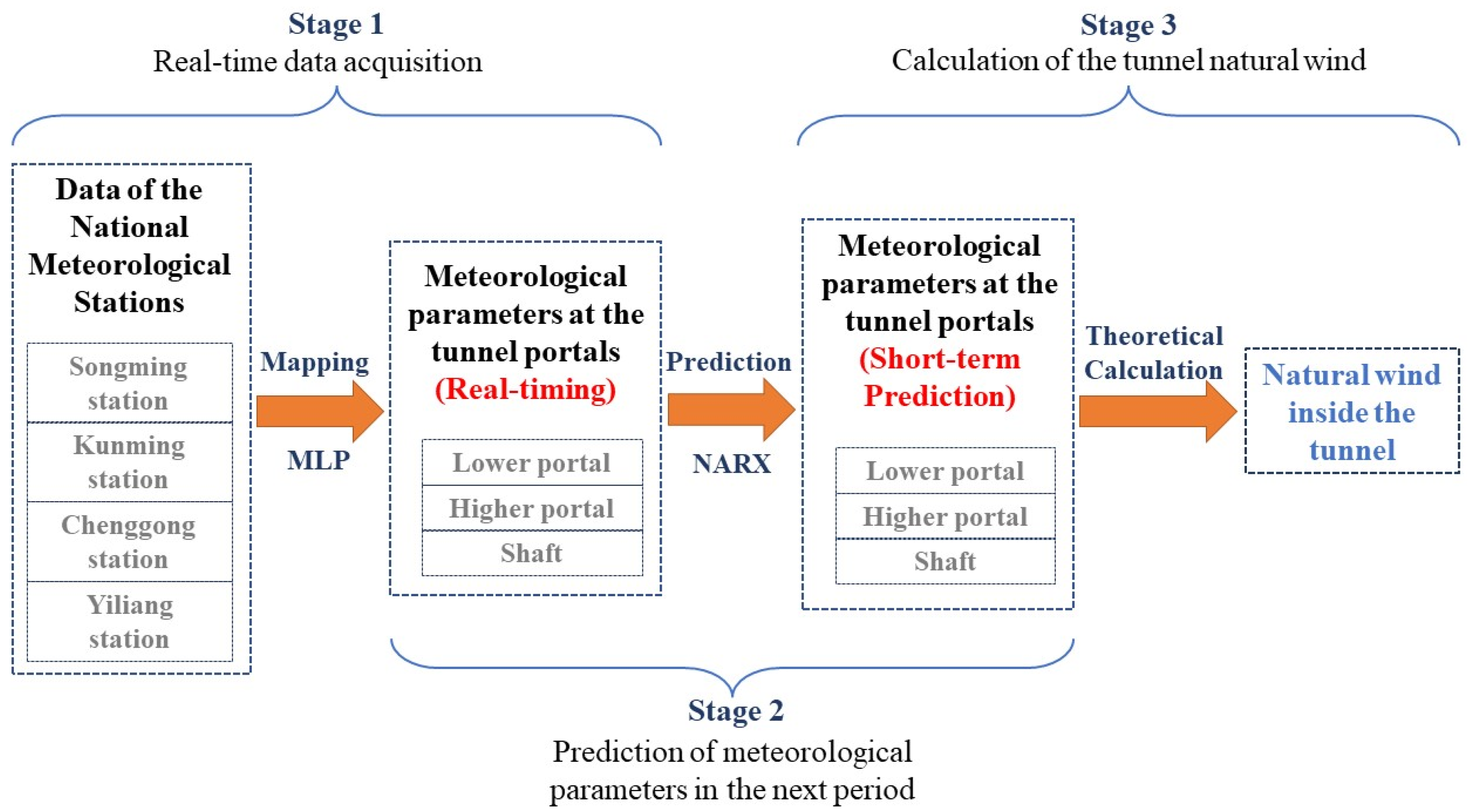
In this paper, the data of the National Meteorological Administration are processed, and a real-time prediction and short-term prediction model are formed for the meteorological parameters of the tunnel portal based on the multi-layer perceptron model (MLP) and nonlinear autoregressive model (NARX). Consequently, the natural wind speed in the tunnel can be obtained by a set of natural wind calculation methods using the predicted data. The purpose of energy saving relying on the fan regulation of Yanglin Tunnel through feedforward ventilation can be realized.

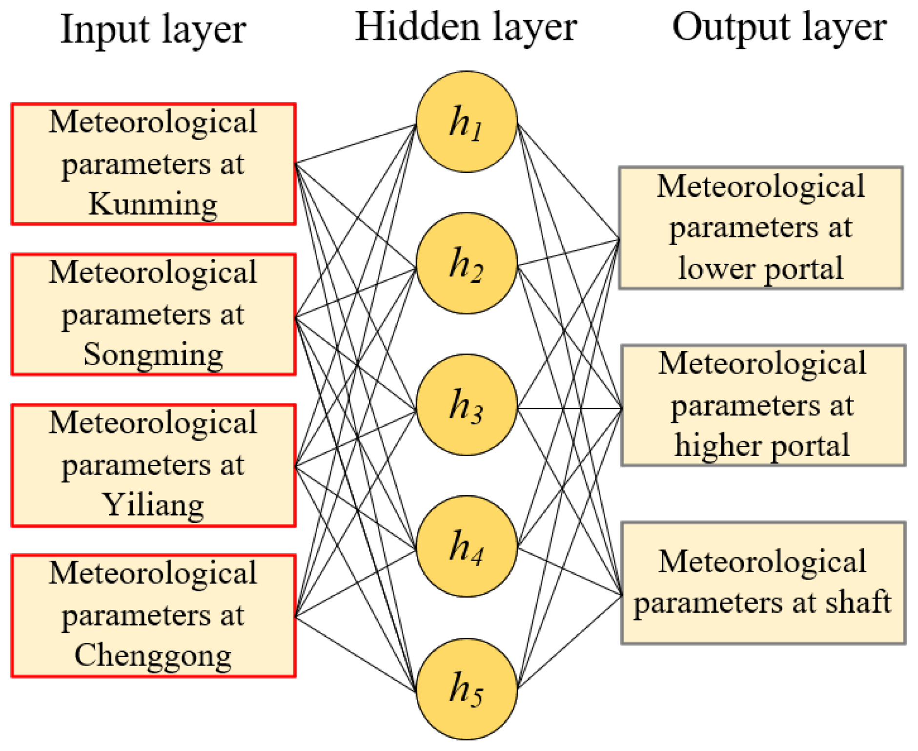
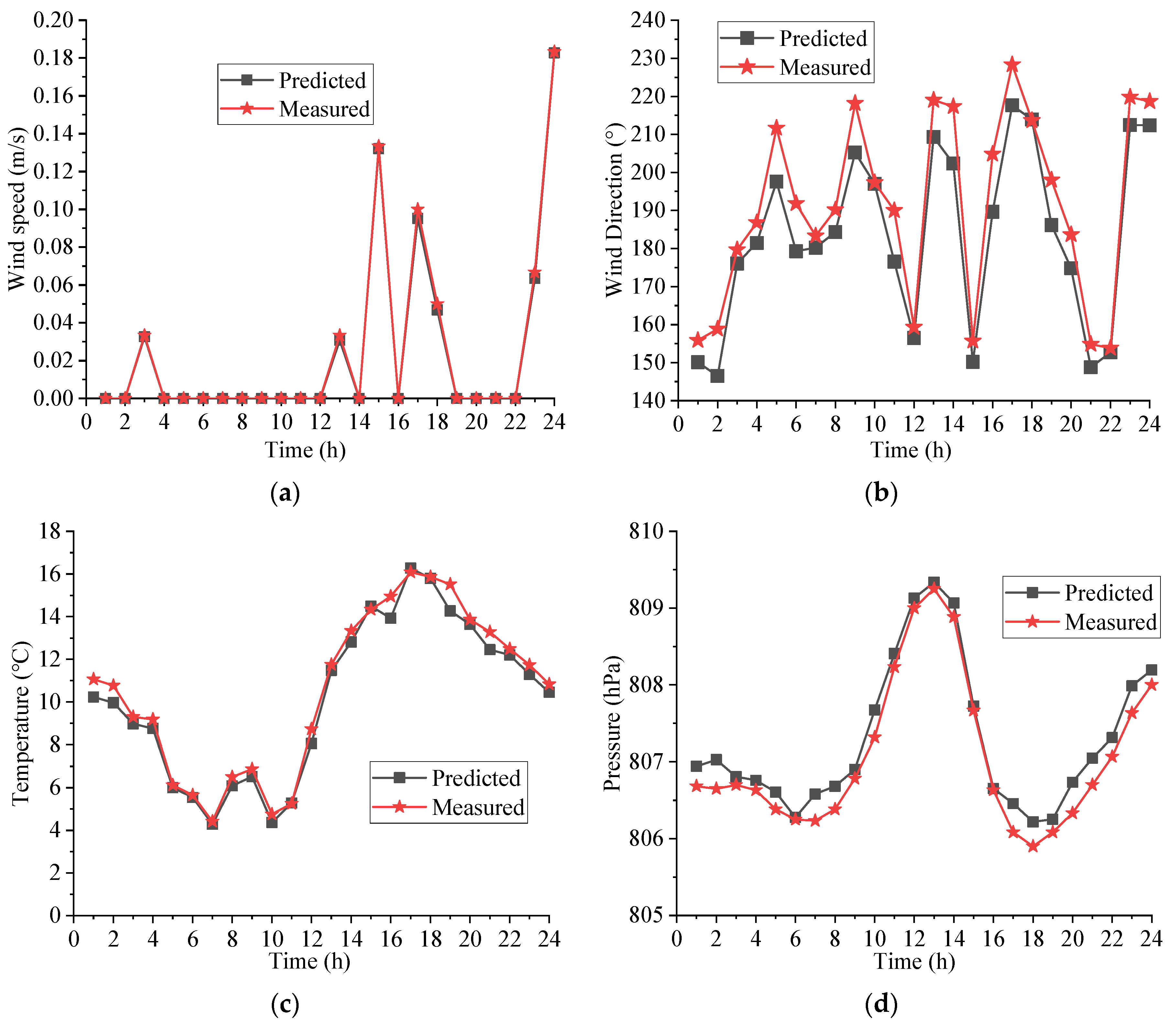
To our knowledge, this study is the first attempt to use the data of the national meteorological stations to map the meteorological parameters of the tunnel portal due to its discontinuous and insufficient nature. As shown in Figure 8, the prediction curves of the five meteorological parameters mapped by MLP all maintain a good, consistent trend with the measured data, and the difference between the predicted value and the measured value is very small. As shown in Table 2, each tunnel portal meteorological station has a strong correlation with several national meteorological stations. Consequently, the prediction accuracy of the MLP model is relatively higher compared with similar studies [27,28].

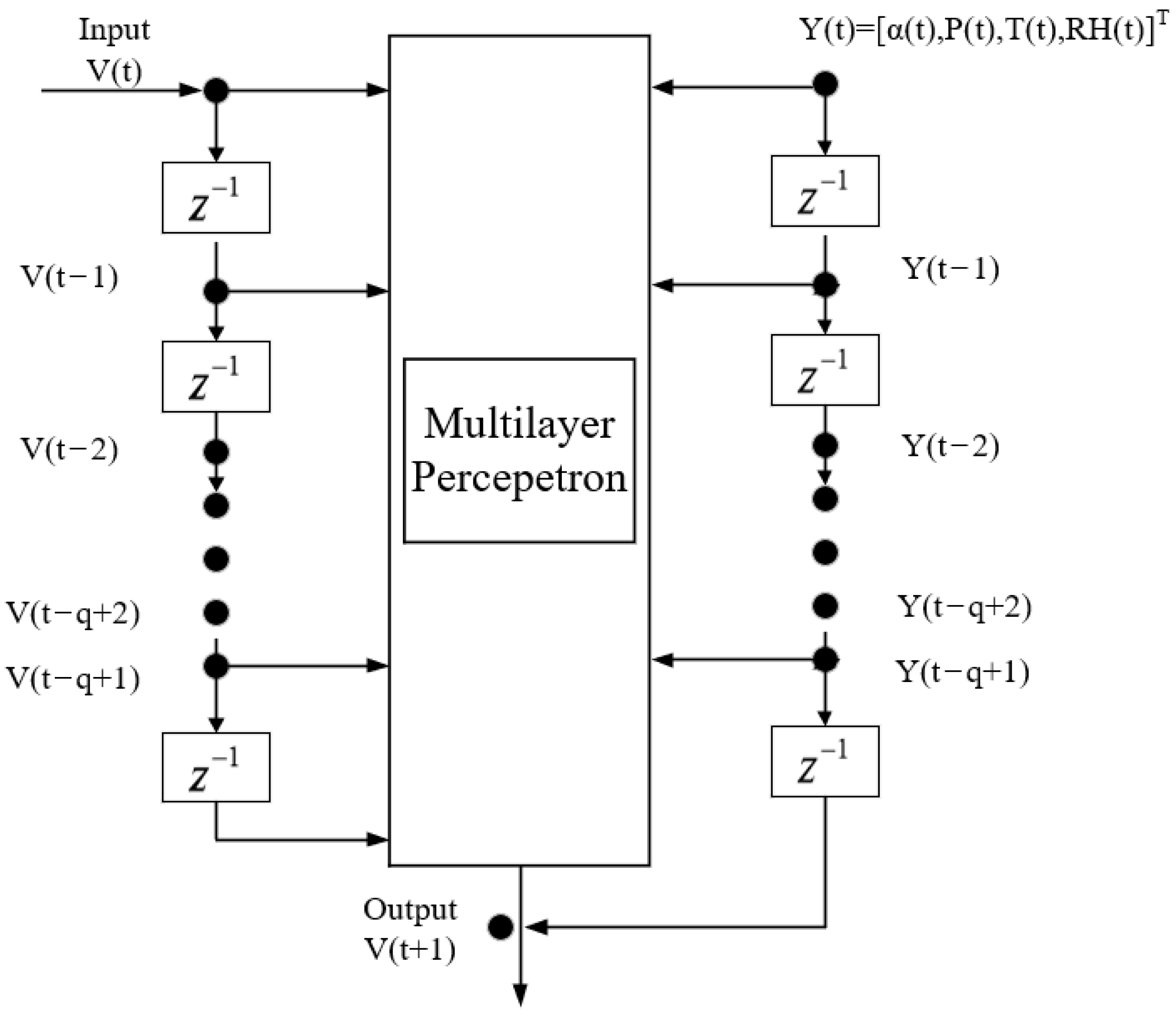
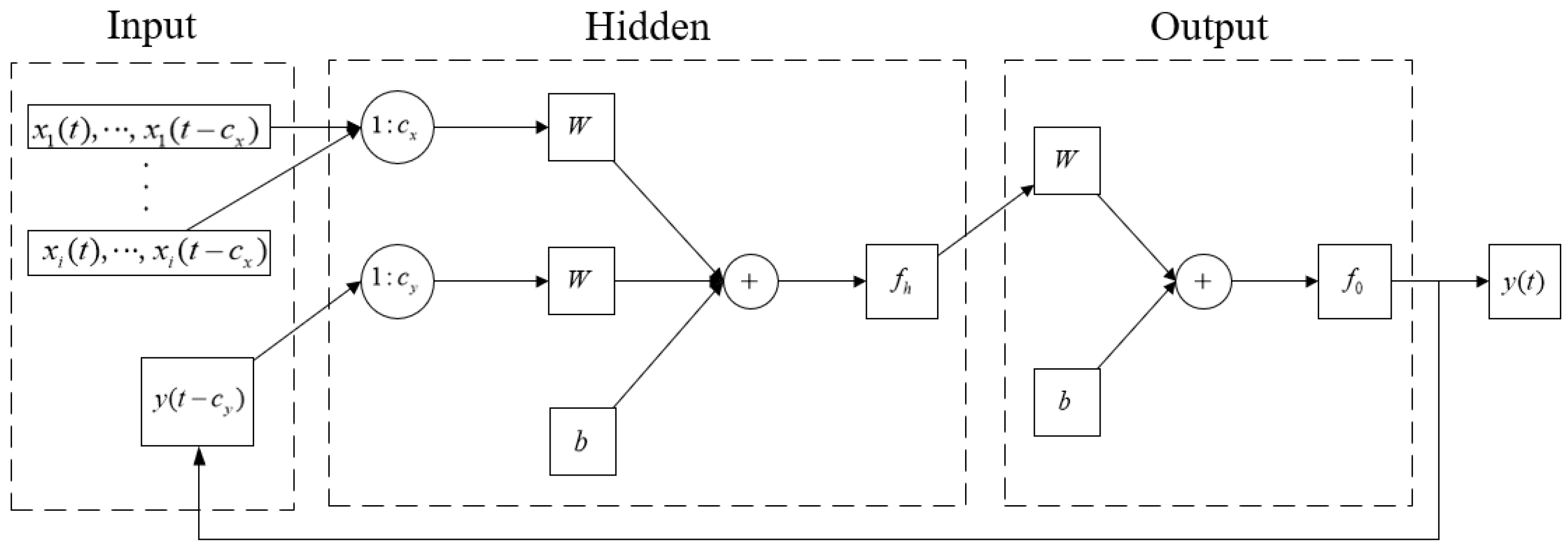
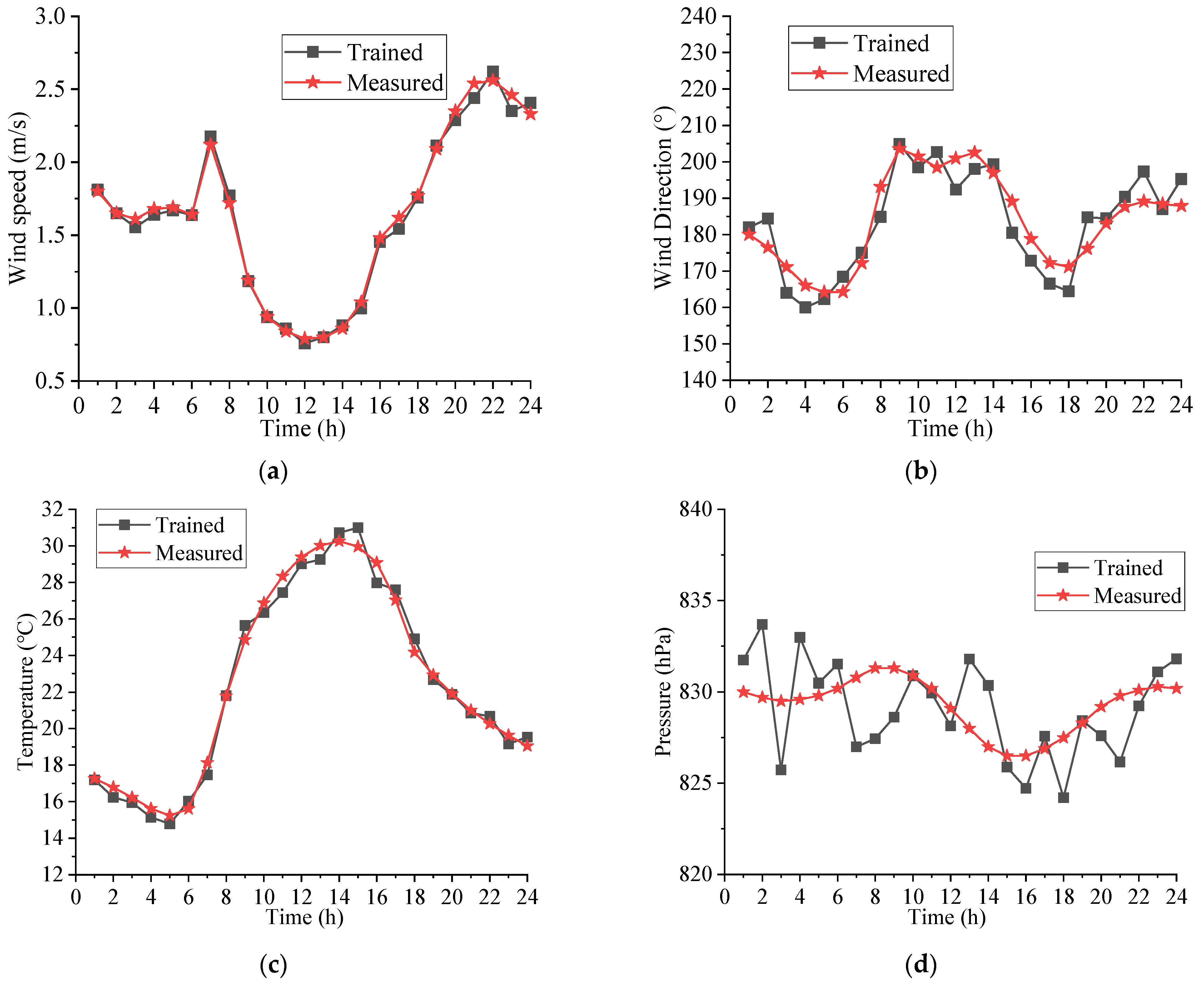
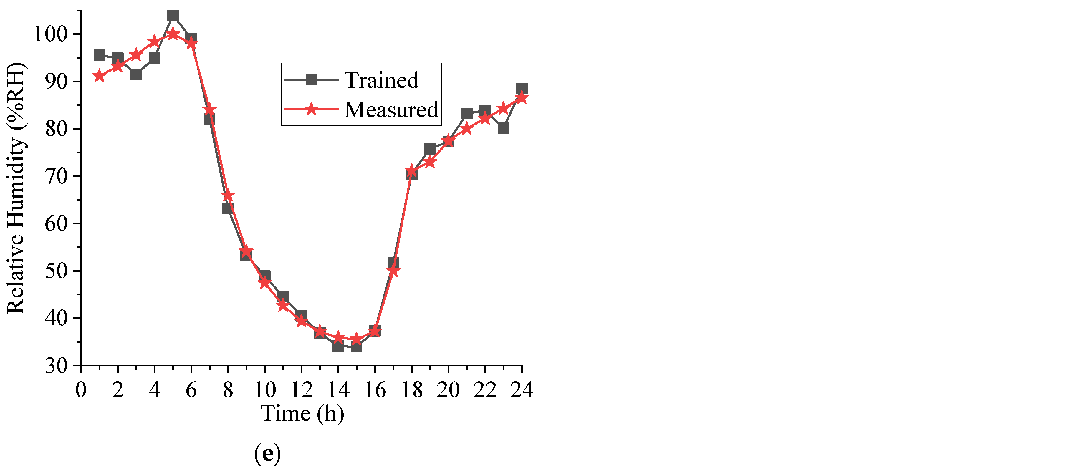
A previous study has shown that contemporary prediction methods fail to maintain a high level of prediction accuracy as the number of steps increases [29]. However, this paper used the existing data of the tunnel portal meteorological stations to revise the predicted data of the MLP model, which preserved the accuracy of the prediction result. As shown in Figure 9, the training values of the five meteorological parameters predicted by the NARX model fit well with the measured curves, showing the same trend. The error values of other parameters are small, except for barometric atmospheric pressure, which is caused by the instability of the model. According to Table 7, the RMSE and MSE of each dataset of the NARX model are controlled within 1.08 and 1.03, respectively, which is comparable to existing studies [22,24].

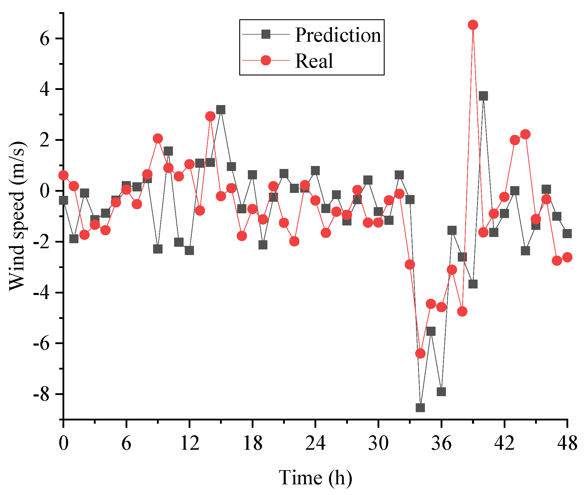
Many scholars have formed a set of effective methods to calculate the natural wind in tunnels. Their work mainly started with the improvement of calculation parameters and methods, focusing on how to calculate the natural wind speed through meteorological parameters more accurately [9,12,14] and lacking research on natural wind prediction. However, the ultimate purpose of using tunnel natural wind is to adjust the output power of the tunnel fan according to the natural wind speed. If the speed and direction of the tunnel natural wind can be calculated based on short-term prediction, the power of the tunnel fan can be prepensely controlled. 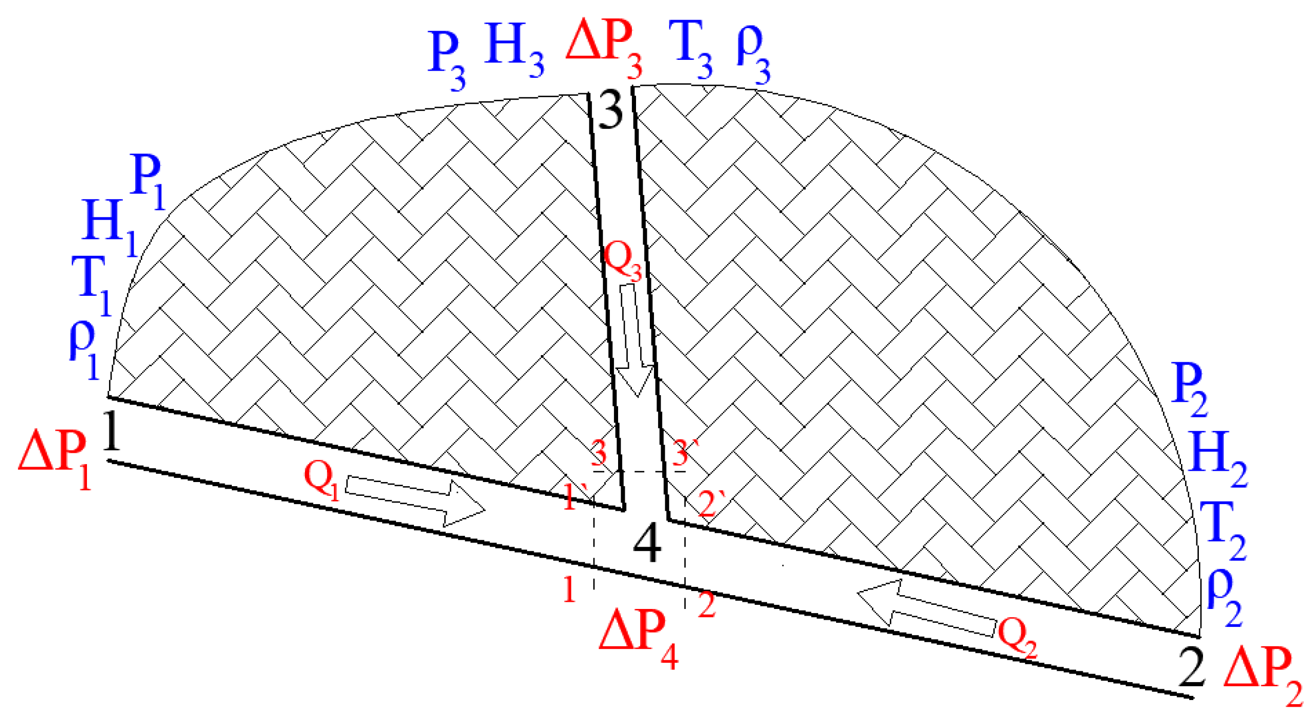As shown in Figure 10, the final predicted natural wind speed in the tunnel also shares the same trend as the measured value. It can be seen that, due to the steps of prediction and theoretical calculation, the final predicted natural wind curve deviates more from the measured value curve, which also leads to a smaller correlation coefficient R. However, this is still within the acceptable range. According to Table 8, the RMSE and MSE of the ultimate tunnel natural wind results are controlled in 0.45 and 0.9, respectively, which confirmed the feasibility of the prediction method.

However, since the focus of this paper is to combine wind speed prediction and tunnel natural wind theoretical calculation, there is a lack of research in the comparison and selection of prediction models to further improve the prediction schedule, such as improving the model algorithm [30] or optimizing the number of neurons [31,32]. In addition, the natural wind calculation method adopted in this paper is relatively conventional. The result will be more accurate if the wind pressure coefficient is calculated by means of a model test or numerical simulation [9].

There are two aspects of this research that can be further discussed in the future. The first is that when the natural wind speed in the tunnel is determined, the most economical and energy-saving ventilation scheme can be explored by changing the control mode of the tunnel fan. The second is to improve the prediction model and algorithm, compare the prediction accuracy and error of different models, and select the prediction method with the best effect.

5. Conclusions

In order to solve the problem of the huge energy consumption of highway tunnel operation ventilation caused by the lack of a tunnel natural wind prediction method, this paper carried out the natural wind ventilation optimization research based on Yanglin Tunnel. By means of theoretical analysis, field testing, software programming, and other methods, the characteristics of the meteorological parameters of Yanglin Tunnel and the prediction method of the tunnel natural wind are studied. Based on the open-source meteorological parameters of the national meteorological station, a set of three-stage prediction methods of tunnel natural wind using MLP, the NARX model, and cyclic calculation methods of ultrastatic pressure difference is proposed. Compared with the field test data, the ultimate prediction results achieved a relatively high accuracy, which could guide the setting of the energy-saving operation ventilation system of Yanglin Tunnel.

References

1. Editorial Department of China Journal of Highway and Transport. Review on China’s Traffic Tunnel Engineering Research: 2022. China J. Highw. Transp. 2022, 35, 1–40. [Google Scholar]
2. Guo, C.; Wang, M.N.; Yang, L.; Sun, Z.T.; Zhang, Y.L.; Xu, J.F. A review of energy consumption and saving in extra-long tunnel operation ventilation in China. Renew. Sustain. Energ. Rev. 2016, 53, 1558–1569. [Google Scholar] [CrossRef]
3. Ministry of Communications of PRC. Guidelines for Design of Ventilation of Highway Tunnels (JTG/T D70/2-02-2014); China Communications Press: Beijing, China, 2014; pp. 37–39. (In Chinese)
4. Tao, L.L.; Ren, X.C.A.; Zhao, D.X.; Zeng, Y.H.; Zhou, X.H. Numerical study on effect of natural wind and piston wind on anti-freezing length of tunnels with high geo-temperature in cold region. Int. J. Therm. Sci. 2022, 172, 11. [Google Scholar] [CrossRef]
5. Yang, C.Q.; Luo, W.H.; Liu, Y.B.; Gao, R.; Zhang, S.K.; Li, A.G.; Du, W.Y.; Zhang, B.; Zhang, J.S. A novel type of unpowered air curtain at a tunnel portal to reduce the intrusion of cold air. Build. Environ. 2022, 218, 12. [Google Scholar] [CrossRef]
6. van Hooff, T.; Blocken, B. Full-scale measurements of indoor environmental conditions and natural ventilation in a large semi-enclosed stadium: Possibilities and limitations for CFD validation. J. Wind Eng. Ind. Aerodyn. 2012, 104, 330–341. [Google Scholar] [CrossRef]
7. Yang, A.S.; Wen, C.Y.; Juan, Y.H.; Su, Y.M.; Wu, J.H. Using the central ventilation shaft design within public buildings for natural aeration enhancement. Appl. Therm. Eng. 2014, 70, 219–230. [Google Scholar] [CrossRef]
8. Chen, T.; Li, Y.Z.; Luan, D.; Jiao, A.; Yang, L.L.; Fan, C.G.; Shi, L. Study of flow characteristics in tunnels induced by canyon wind. J. Wind Eng. Ind. Aerodyn. 2020, 202, 12. [Google Scholar] [CrossRef]
9. Wang, M.N.; Tian, Y.; Yu, L.; Wang, X.; Zhang, Z.H.; Yan, G.F. Research on the wind pressure coefficient in natural wind calculations for extra-long highway tunnels with shafts. J. Wind Eng. Ind. Aerodyn. 2019, 195, 12. [Google Scholar] [CrossRef]
10. Krol, M.; Krol, A.; Koper, P.; Wrona, P. The influence of natural draught on the air flow in a tunnel with longitudinal ventilation. Tunn. Undergr. Space Technol. 2019, 85, 140–148. [Google Scholar] [CrossRef]
11. Guo, C.; Xu, J.F.; Yang, L.; Guo, X.; Zhang, Y.L.; Wang, M.N. Energy-Saving Network Ventilation Technology of Extra-Long Tunnel in Climate Separation Zone. Appl. Sci. 2017, 7, 20. [Google Scholar] [CrossRef] [Green Version]
12. Zhang, Z.Q.; Zhang, H.; Tan, Y.J.; Yang, H.Y. Natural wind utilization in the vertical shaft of a super-long highway tunnel and its energy saving effect. Build. Environ. 2018, 145, 140–152. [Google Scholar] [CrossRef]
13. Mao, J.F.; Huang, Y.L.; Zhou, J.; Xing, Z.L. Energy-saving and Economic study of Natural Ventilation in city tunnel. In Proceedings of the 2nd International Conference on Civil Engineering, Architecture and Building Materials (CEABM 2012), Yantai, China, 25–27 May 2012; pp. 92–97. [Google Scholar]
14. Wang, Y.D.; Zheng, R.J.; Bai, W.J.; Qin, Z.J.; Chai, L.L.; Wan, S.T.; Yan, S. Study on the utilization of non-mechanical ventilation power in extra-long highway tunnels with shafts. J. Wind Eng. Ind. Aerodyn. 2022, 221, 10. [Google Scholar] [CrossRef]
15. Jung, J.; Broadwater, R.P. Current status and future advances for wind speed and power forecasting. Renew. Sustain. Energ. Rev. 2014, 31, 762–777. [Google Scholar] [CrossRef]
16. Li, G.; Shi, J. On comparing three artificial neural networks for wind speed forecasting. Appl. Energy 2010, 87, 2313–2320. [Google Scholar] [CrossRef]
17. Zhao, P.; Wang, J.F.; Xia, J.R.; Dai, Y.P.; Sheng, Y.X.; Yue, J. Performance evaluation and accuracy enhancement of a day-ahead wind power forecasting system in China. Renew. Energy 2012, 43, 234–241. [Google Scholar] [CrossRef]
18. Shi, J.; Ding, Z.H.; Lee, W.J.; Yang, Y.P.; Liu, Y.Q.; Zhang, M.M. Hybrid Forecasting Model for Very-Short Term Wind Power Forecasting Based on Grey Relational Analysis and Wind Speed Distribution Features. IEEE Trans. Smart Grid 2014, 5, 521–526. [Google Scholar] [CrossRef]
19. Bastos, B.Q.; Oliveira, F.L.C.; Milidiu, R.L. U-Convolutional model for spatio-temporal wind speed forecasting. Int. J. Forecast. 2021, 37, 949–970. [Google Scholar] [CrossRef]
20. Sacie, M.; Santos, M.; Lopez, R.; Pandit, R. Use of State-of-Art Machine Learning Technologies for Forecasting Offshore Wind Speed, Wave and Misalignment to Improve Wind Turbine Performance. J. Mar. Sci. Eng. 2022, 10, 18. [Google Scholar] [CrossRef]
21. de Paiva, G.M.; Pimentel, S.P.; Alvarenga, B.P.; Marra, E.G.; Mussetta, M.; Leva, S. Multiple Site Intraday Solar Irradiance Forecasting by Machine Learning Algorithms: MGGP and MLP Neural Networks. Energies 2020, 13, 28. [Google Scholar]
22. Cadenas, E.; Rivera, W.; Campos-Amezcua, R.; Heard, C. Wind Speed Prediction Using a Univariate ARIMA Model and a Multivariate NARX Model. Energies 2016, 9, 15. [Google Scholar] [CrossRef] [Green Version]
23. Di Nunno, F.; de Marinis, G.; Gargano, R.; Granata, F. Tide Prediction in the Venice Lagoon Using Nonlinear Autoregressive Exogenous (NARX) Neural Network. Water 2021, 13, 19. [Google Scholar] [CrossRef]
24. Calik, H.; Ak, N.; Guney, I. Artificial NARX Neural Network Model of Wind Speed: Case of Istanbul-Avcilar. J. Electr. Eng. Technol. 2021, 16, 2553–2560. [Google Scholar] [CrossRef]
25. Shabin, M.A.; Maier, H.R.; Jaksa, M.B. Data division for developing neural networks applied to geotechnical engineering. J. Comput. Civil. Eng. 2004, 18, 105–114. [Google Scholar]
26. Qiao, D.L.; Wu, S.; Li, G.; You, J.X.; Zhang, J.; Shen, B.L. Wind speed forecasting using multi-site collaborative deep learning for complex terrain application in valleys. Renew. Energy 2022, 189, 231–244. [Google Scholar] [CrossRef]
27. Velo, R.; Lopez, P.; Maseda, F. Wind speed estimation using multilayer perceptron. Energy Conv. Manag. 2014, 81, 1–9. [Google Scholar] [CrossRef]
28. Bulut, M.; Tora, H.; Buaisha, M. Comparison of Three Different Learning Methods of Multilayer Perceptron Neural Network for Wind Speed Forecasting. Gazi Univ. J. Sci. 2021, 34, 439–454. [Google Scholar] [CrossRef]
29. Rana, M.; Rahman, A. Multiple steps ahead solar photovoltaic power forecasting based on univariate machine learning models and data re-sampling. Sustain. Energy Grids Netw. 2020, 21, 12. [Google Scholar] [CrossRef]
30. Yeh, W.C.; Yeh, Y.M.; Chang, P.C.; Ke, Y.C.; Chung, V. Forecasting wind power in the Mai Liao Wind Farm based on the multi-layer perceptron artificial neural network model with improved simplified swarm optimization. Int. J. Electr. Power Energy Syst. 2014, 55, 741–748. [Google Scholar] [CrossRef]
31. Madhiarasan, M.; Deepa, S.N. Comparative analysis on hidden neurons estimation in multi layer perceptron neural networks for wind speed forecasting. Artif. Intell. Rev. 2017, 48, 449–471. [Google Scholar] [CrossRef]
32. Cadenas, E.; Rivera, W.; Campos-Amezcua, R.; Cadenas, R. Wind speed forecasting using the NARX model, case: La Mata, Oaxaca, Mexico. Neural Comput. Appl. 2016, 27, 2417–2428. [Google Scholar] [CrossRef]
Figure 1. Geographical location map of the four national stations and tunnel portals.
Processes 11 00224 g001
Figure 2. Three stages of tunnel natural wind prediction processes.
Processes 11 00224 g002
Figure 3. Multi-layer perceptron structure for real-time data acquisition.
Processes 11 00224 g003
Figure 4. Data flow of the MLP after the input.
Processes 11 00224 g004
Figure 5. General NARX model structure.
Processes 11 00224 g005
Figure 6. NARX grid structure for wind speed prediction.
Processes 11 00224 g006
Figure 7. Schematic diagram of the tunnel section with a shaft.
Processes 11 00224 g007
Figure 8. Curves of the predicted and measured data. (a) Wind speed. (b) Wind direction. (c) Temperature. (d) Barometric pressure. (e) Relative humidity.
Processes 11 00224 g008aProcesses 11 00224 g008b
Figure 9. Comparison between the trained and measured results. (a) Wind speed. (b) Wind direction. (c) Temperature. (d) Barometric pressure. (e) Relative humidity.
Processes 11 00224 g009aProcesses 11 00224 g009b
Figure 10. Comparison between the predicted and measured natural wind speed.
Processes 11 00224 g010