Article

Applications of Fractional Partial Differential Equations for MHD Casson Fluid Flow with Innovative Ternary Nanoparticles

1
Department of Mathematics, University of Management and Technology, Lahore 54770, Pakistan
2
Department of Mathematics, Division of Science and Technology, University of Education, Lahore 54000, Pakistan
3
Department of Mathematics, Dawood University of Engineering and Technology, Karachi 74800, Pakistan
4
Center of Research, Faculty of Engineering and Technology, Future University in Egypt, New Cairo 11835, Egypt
*
Author to whom correspondence should be addressed.
Processes 2023, 11(1), 218; https://doi.org/10.3390/pr11010218
Submission received: 8 December 2022 / Revised: 23 December 2022 / Accepted: 28 December 2022 / Published: 10 January 2023
(This article belongs to the Section Materials Processes)

Abstract

:
This study deals with the modeling issues of the transport problem with a fractional operator. The fractional model with generalized Fourier’s law is discussed for Casson fluid flow over a flat surface. The dimensionless governing model is solved with the Laplace transform method, and the different comparisons are plotted from the obtained solutions. Other features of the problem have been analyzed instead of the symmetric behavior of the properties for different values of the fractional parameter. As a result, the ternary nanoparticles approach can be used to improve the fluid properties better than hybrid and mono nanoparticles. Further, it is evident that the law-based fractional model is more accurate and efficient in fitting any experimental data instead of an artificial replacement.

1. Introduction

Fractional calculus theory has received more attention from scholars during the past few decades in a number of disciplines. Indeed, it has been established that the usage of fractional derivatives is quite advantageous in modifying many processes connected to thermal transport, engineering sciences, circuit analysis, biotechnology, and signal processing. Many further applications of heat and mass transfer and fluid dynamics can be found in the references [1,2,3,4,5]. Typically, these models are expressed in terms of classic integer-order partial differential equations (PDEs). Traditional PDEs, on the other hand, are incapable of decoding the complicated behavior of physical flow parameters and memory effects. The classical calculus is so named because it measures the immediate rate of change of the output when the input level changes. As a result, it cannot incorporate the prior state of the system, which is known as the memory effect. However, using fractional calculus (FC), the rate of change is influenced by each point in the interval under consideration, allowing for the incorporation of any system’s prior history or memory effects. Jagdev et al. [6], Kolade and Atangana. [7], and Baleanu et al. [8] have all published books on fractional derivatives that cover both the use of fractional derivatives and their operators.
Ordinary life problems typically have arbitrary boundary conditions. It is possible to research scenarios in which the temperature of the wall varies in phases. Such topics are being researched diligently by researchers. Many engineering and industrial procedures rely on the flow of heat in fluids, including nuclear operations, gas turbines, heating and cooling processes, device design, and the management of high-tech thermal systems. Studies of the flow of MHD nanoparticles with ramping concentration and temperature conditions in the literature are not currently investigated analytically in depth due to the difficulties of the relationships. Hayday et al. [9], Schetz. [10], and Malhotra et al. [11] pioneered the notion of ramping temperature. Ramping heat is most commonly used to vaporise cancer cells during thermal treatment. Temperature spikes produced by natural sources are mitigated by ramped conditions [12]. Das et al. [13] examined how step wise heating affected the flow of an incompressible, optically thin fluid over a plate. According to ramping and constant boundary conditions, Nandkeolyar et al. [14] examined and compared MHD natural convection flow and different plate motions at uniform velocity, periodic acceleration, and single acceleration. Mass and heat transfer on a vertical plate were explored by Seth et al. [15,16,17,18] in the presence of increasing concentration and temperature, chemical reaction, heat absorption, Darcy’s law, thermal radiation, porous material, and Hall current, among other characteristics. Zin et al. [19] focused on the impact of ramping temperature, Jeffrey Fluid Flow’s spontaneous convection, and the effects of heat radiation and magnetic fields. Indian mathematician Tilak Raj Prabhakar, known as the creator of the Prabhakar work, first suggested that the Mittag-Leffler function can be expanded to three parameters in 1971. In order to choose pleasing numerical models that arrive at a fair compromise between hypothetical and experimental results, Prabhakar administrators with defined fractional coefficients may be a valuable tool [20,21]. Elnaqeeb et al. [22] investigated Prabhakar-like heat transfer in a carbon nanotube nanoparticle with natural convection flow. Shah et al.’s [23] investigation focused on the spontaneous convection streams and generalized thermal transport of Prabhakar-like fractional Maxwell fluids. Eshaghi et al. [24] regularized the dynamics and stability of integrodifferential and neutral Prabhakar fractional differential systems. The Prabhakar fractional model was employed to analyze the thermal behavior of a viscous carbon nanotube nanoparticle in free convection flows with generalized thermal transport, as termed by Tanveer et al. [25]. Alidousti [26] uses the Prabhakar derivative and a stable field to research fractional differential classifications. Derakhshan [27] established a novel numerical strategy for the solution of variable-order fractional integrodifferential equations within the framework of Hilfer Prabhakar derivatives. In a convection channel containing hybrid nanoparticles, Prabhakar fractional derivatives of non-Newtonian fluid were investigated by Asjad et al. [28]. The Effect of Newtonian Heating through Fourier and Fick’s Laws on the Thermal Transport of an Oldroyd-B Fluid Using a Generalized Mittag-Leffler Kernel was covered by the authors of [29]. The unstable flow of thermal transfer Prabhakar types generalize Casson’s nanoparticle. The Mittage-Leffler kernel was studied by Wang et al. [30]. The generalized Mittag-Leffler input stability of the fractional differential equation was covered by Sene and Srivastava [31]. Recent investigations have found that nanoparticles are better at transferring heat than regular fluids. The main applications of hybrid nanoparticles in real life are solar energy refrigeration and heating, ventilation, air conditioning, heat exchangers, heat pipes, coolants in machining and manufacturing, ships, defense, nuclear system cooling, and the automotive industry. Therefore, switching from regular fluids to nanoparticles makes sense. Numerous researchers are interested in studying nanoparticles because of their enhanced heat capacity. In addition to biology, electronics, transportation, and food, they have a big influence on many different industrial domains. Nanoparticles are very tiny particles that increase the conductivity of base fluids when they are introduced to them. The primary components of nanoparticles are X 2 O 3 (metal oxide), carbon tubes, N 3 (nitride), metal, and CaC 2 carbide [32]. Reddy et al. [33] evaluated the performance of MgO (magnesium oxide) and MoS 2 (molybdenum disulfide) nanoparticles in a micropolar thermal flux model. Due to the extensive study of the aforementioned fluid, the thorough blending of conventional fluids with two distinct types of nanomaterials has been named hybrid nanoparticles. The thermal performance of hybrid nanoparticles is assessed using thermal conductivities, heat, and molecular density concentrations, as well as nanoparticle thickness and size. The thermal conductivity of hybrid nanoparticles may be determined using any method or formula. Jamei et al. [34] reported the conjugate heat-transfer assessment for ethylene glycol base hybrid nanoliquids. Ti O 2 and graphene nanoparticles were combined with purified water by Xian et al. [35] to produce powerful hybrid nanoliquids. Through the use of an expanded surface, Arani and Aberoumand [36] looked into the numerical estimation of the mobility of Ag + CuO / H 2 O hybrid nanoparticles at their stagnation point. The motion and energy transmission of Cu+ Al 2 O 3 /water hybrid nanoparticles through a spinning drum were investigated by Roy et al. [37] for both assistive and resistive motions. The ternary hybrid nanoparticle, a homogeneous blend of three different nanomaterial types with a special base liquid, was very recently developed. The findings of a few research studies, however, seem to be intriguing and instructive. The intricate processes of CuO , MgO , and TiO 2 movement in H 2 O were studied by Mousavi et al. [38].
In general, ternary hybrid nanoparticles resemble Newtonian liquids in their physical characteristics. At higher temperatures, tri-hybrid nanoparticle concentrations are correspondingly lower. The thermal performance of water-based ternary hybrid nanoparticles with diverse shapes (spherical, cylindrical, and platelet) is high for radiator cooling. If the radiator is built utilizing new ternary hybrid nanoparticle principles, the temperature of the engines may be raised, extending the life of the machinery. The heat capacity of the typical functional fluid may be increased by adding different kinds of nanoparticles. The thermophysical characteristics of a ternary hybrid nanoparticle consisting of TiO 2 and Al 2 O 3 in water at 35 to 50 C were studied by Sahoo and Kumar [39]. Time-fractal-fractional stochastic differential equations with the fractal fractional differential operator of Atangana under the meaning of Caputo and with a kernel of the power law type were studied by Xia et al. [40]. The analysis and optimal control of j-Hilfer fractional semilinear equations involves non-local impulsive conditions [41]. Other researchers have expressed interest in the related published work on ternary hybrids and on mono nanoparticles, including Manjunatha et al. [42], Nazir et al. [43], Nasir et al. [44], Guedri et al. [45], Saqib et al. [46], and Irandoost Shahrestani [47].
There was no study that used a fractional operator for an important class of nanoparticles, such as mono nanoparticles, hybrid nanoparticles, and ternary nanoparticles, on a single vertical plate. The researchers were driven to create a concept of existing nanoparticles in order to boost heat transfer since there is a strong demand in the industry for a cooling agent with improved heat transfer capabilities. To describe the channel flow problem, the Prabhakar fractional derivative was used, which included mono, hybrid, and ternary nanoparticles. In order to support the experimental results, a theoretical model for ternary nanoparticles is presented in this study. As a result, the primary goal is to discover analytical solutions for energy and momentum using the Laplace transform method and parametric analysis to illustrate the flexibility of the proposed model. The governing equations are obtained by introducing the dimensionless variables. The Prabhakar fractional derivative operator was used to find the fractional model of nanofluids with kerosene oil base fluid. Due to higher thermal conductivities, copper and aluminum oxide are considered as the nanoparticles. We find the solutions of temperature and velocity with the help of the Laplace transform. Using Mathcads software, analytical solutions are designed graphically for fractional and flow parameters. The thermo-physical properties of nanoparticles and the base fluid are given in Table 1.

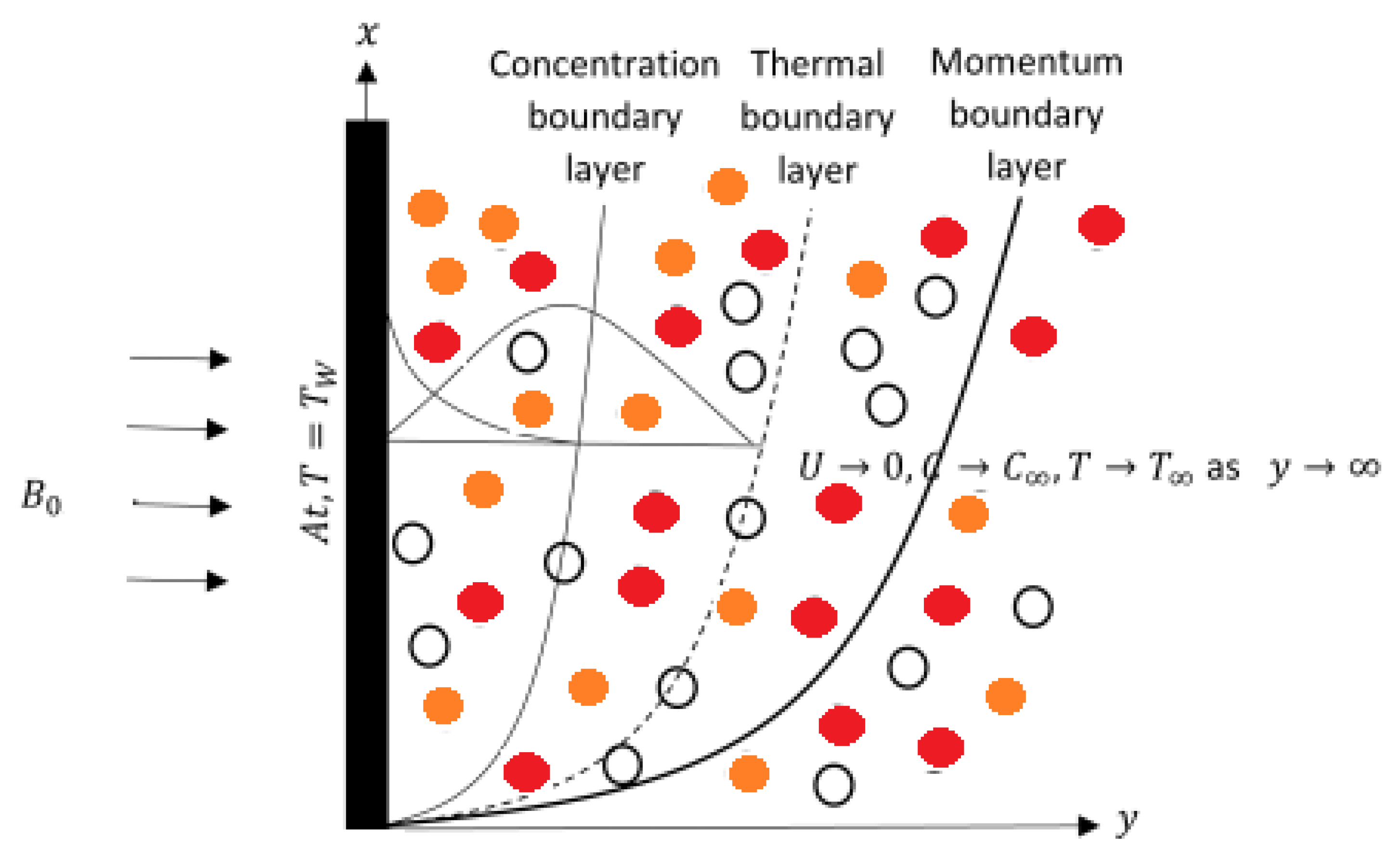
2. Mathematical Formulation

The significance of magnetic flux of nanoparticles discharge over an accelerating plate having a non-linear thermal radiative flux as shown in Figure 1. The thermodynamic effect of the fluid and the motion of the plate are both constant at a time t = 0. The temperature distribution and the volume fraction far from the surface of the plate are T and C , which are referred to as the ambient temperature and volume fraction. As the time t 0 , the fluid of the plate begins to accelerate and the temperature of the wall rises. A permeating homogeneous magnetic filled B 0 is applied to the fluid parallel to the y axis. The effects of an induced magnetic field in a fluid flow are ignored due to the tiny Reynolds number. The effects of a magnetic field that is produced in a fluid flow are negligible due to the low Reynolds number. When the Reynolds number is high, the effects of a magnetic field can be significant. Fluid flow is constrained at y > 0 when the y coordinate is perpendicular to the plate. The variables y and time t influence the velocity U, temperature T, and concentration C.
The momentum equation is [49]
ρ m n f U t = τ y σ m n f B 0 2 U + ρ ( g β T ) m n f ( T T ) + ρ ( g β c ) m n f ( C C ) ,
The relation between shear stress and deformation with Prabhakar fractional derivative
τ = μ m n f ( 1 + 1 β ) C D α , β , a γ U y .
The energy equation for heat flux:
( ρ C p ) m n f T t = q y .
The generalized Fourier’s Law [50] in the form of the Prabhakar fractional derivative:
q = k m n f C D α , β , a γ T y ,
The equation of diffusion:
C t = J y ,
The generalized Fick’s Law [51] for mass diffusibility:
J = D m n f C D α , β , a γ C y .
The initial and boundary conditions are
U ( y , 0 ) = 0 , U ( , t ) = 0 , U ( 0 , t ) = A t , a s y ,
C ( y , 0 ) = C , C ( , t ) = C , C ( 0 , t ) = C w , a s y ,
T ( y , 0 ) = T , T ( , t ) = T , T ( 0 , t ) = T w , a s y .
The relations of ternary nanoparticles are defined as:
μ m n f = μ f ( 1 ( ϕ 1 + ϕ 2 + ϕ 3 ) ) 2.5 , ρ m n f = ( 1 ( ϕ 1 + ϕ 2 + ϕ 3 ) ) ρ f + ϕ 1 ρ s 1 + ϕ 2 ρ s 2 + ϕ 3 ρ s 3
( ρ C p ) m n f = ( 1 ( ϕ 1 + ϕ 2 + ϕ 3 ) ) ( ρ C p ) f + ϕ 1 ( ρ C p ) s 1 + ϕ 2 ( ρ C p ) s 2 + ϕ 3 ( ρ C p ) s 3
( ρ β T ) m n f = ( 1 ( ϕ 1 + ϕ 2 + ϕ 3 ) ) ( ρ β T ) f + ϕ 1 ( ρ β T ) s 1 + ϕ 2 ( ρ β T ) s 2 + ϕ 3 ( ρ β T ) s 3
k h n f k b f = ϕ 1 k 1 + ϕ 2 k 2 + ϕ 3 k 3 + 2 ( ϕ 1 + ϕ 2 + ϕ 3 ) k f + 2 ( ϕ 1 + ϕ 2 + ϕ 3 ) ( ϕ 1 k 1 + ϕ 2 k 2 + ϕ 3 k 3 ) 2 ( ϕ 1 + ϕ 2 + ϕ 3 ) 2 k f ϕ 1 k 1 + ϕ 2 k 2 + ϕ 3 k 3 + 2 ( ϕ 1 + ϕ 2 + ϕ 3 ) k f ( ϕ 1 + ϕ 2 + ϕ 3 ) ( ϕ 1 k 1 + ϕ 2 k 2 + ϕ 3 k 3 ) + ( ϕ 1 + ϕ 2 + ϕ 3 ) 2 k f
Introducing dimensionless parameters from Equation (9)
U * = U ( ν A ) 1 3 , y * = y A 1 3 ν 2 3 , C * = C C C w C , t * = t A 2 3 ν 1 3 ,
T * = T T T w T , q * = q q 0 , J * = J J 0 , τ * = τ τ 0
The dimensionless governing model of Equations (1)–(5) without the asterisk notations
U t = a 4 τ y a 5 M 2 U + a 6 Gr T + a 7 Gm C ,
with non-dimensional shear stress
τ = 1 β 0 C D α , β , a γ U y ,
the dimensionless energy equation
T t = a 1 Pr q y ,
with non-dimensional Fourier’s law
q = a 2 C D α , β , a γ T y .
the dimensionless diffusion equation
C t = 1 Sc J y ,
with non-dimensional Fick’s law
J = a 3 C D α , β , a γ C y .
where,
β 0 = β 1 + β , Gr = g ( β T ) f ( T w T ) A , Gm = g ( β c ) f ( C w C ) A , M 2 = σ f B 0 2 ν 1 3 ρ A 2 3
Pr = ( μ C p ) f k f , Sc = ν D f , a 1 = 1 1 ( ϕ 1 + ϕ 2 + ϕ 3 ) + ϕ 1 ( ρ C p ) s 1 + ϕ 2 ( ρ C p ) s 2 + ϕ 3 ( ρ C p ) s 3 ( ρ C p ) f
τ 0 = μ m n f A 2 3 ν 1 3 , J 0 = D f ( C w C ) A 1 3 ν 2 3 , q 0 = k f ( T w T ) A 1 3 ν 2 3 , a 2 = k m n f k f
a 3 = D m n f D f , a 4 = 1 a 1 ( 1 ( ϕ 1 + ϕ 2 + ϕ 3 ) ) 2.5 , a 5 = σ m n f σ f , a 6 = a 8 a 1 , a 7 = a 9 a 1
a 8 = 1 ( ϕ 1 + ϕ 2 + ϕ 3 ) + ϕ 1 ( ρ β T ) s 1 + ϕ 2 ( ρ β T ) s 2 + ϕ 3 ( ρ β T ) s 3 ( ρ β T ) f ,
a 9 = 1 ( ϕ 1 + ϕ 2 + ϕ 3 ) + ϕ 1 ( ρ β c ) s 1 + ϕ 2 ( ρ β c ) s 2 + ϕ 3 ( ρ β c ) s 3 ( ρ β c ) f .
Initial and boundary conditions that are dimensionless,
T ( 0 , t ) = 1 , T ( y , 0 ) = 0 , T ( , t ) = 0 ,
U ( 0 , t ) = t , U ( y , 0 ) = 0 , U ( , t ) = 0 ,
C ( 0 , t ) = 1 , C ( y , 0 ) = 0 , C ( , t ) = 0 .

3. Preliminaries of Fractional Calculus

Definition 1.
The Prabhakar Kernal. For t ϵ R ,
e α , β γ ( a ; t ) = t β 1 E α , β γ ( a t α ) , α , β , γ ε C , R e ( α ) > 0 ,
is called the Prabhakar kernel [52].
Definition 2.
(The Prabhakar integral). For t ϵ ( 0 , b ) and a function hϵ L 1 ( 0 , b )
E α , β , a γ h ( t ) = h ( t ) e α , β γ ( a ; t ) = 0 t h ( τ ) ( t τ ) β 1 E α , β γ ( a ( t τ ) ) α d τ
is known as the Prabhakar integral. The LT (Laplace transform) of Equation (21) is given [52],
L { E α , β , a γ h ( t ) } ( s ) = L { h ( t ) } L { e α , β γ ( a ; t ) } = L { h ( t ) } s a γ β ( s α a ) γ
Definition 3.
The Prabhakar derivative.
Let gε L 1 ( 0 , b ) and τε ( 0 , b ) , then for m = [ v ] .
( D α , ν , β , a + g γ ) = ( d m d t m ( E α , n , ν , β , a + g γ ) ) ( τ ) ,
where α , β , γ , ν are the elements of complex number C [52].
Definition 4.
The regularized Prabhakar derivative.
Let 0 < β n , where n belongs to Z and h ε A C n ( 0 , b ) . The regularized derivative is defined as [52,53]
C D α , β , a γ h ( t ) = h ( n ) ( t ) E α , n β , a γ = h n ( t ) e α , n β γ ( a ; t ) ,
= 0 t h n ( τ ) ( t τ ) n β 1 E α , n β γ ( a ( t τ ) α ) d τ ,
where h ( n ) represents the nth differential of h ( t ) and A C n ( 0 , b ) represents the set of functions h ( t ) with real values. The Laplace transform of the Equation (24) is given by
L ( C D α , β , a γ h ( t ) ) = L { h ( n ) ( t ) e α , n β γ } ,
= L { h ( n ) ( t ) } L { e α , n β γ ( a ; t ) } ,
= s β n ( 1 a s α ) γ L { h ( n ) ( t ) } .

4. Solution of the Problem Based on Generalized Law with Ternary Nanoparticles

The Prabhakar fractional derivative and the Laplace transform approach are used to calculate the temperature and concentration solution. Our main purpose is to determine the velocity field for the Casson fluid.

4.1. Computation of Temperature Field

Using Laplace transform to solve Equations (12) and (13)
s T ¯ ( y , s ) = a 1 Pr q ¯ ( y , s ) y ,
q ¯ ( y , s ) = a 2 s β ( 1 a s α ) γ T ¯ y .
By introducing Equation (27) into (26)
2 T ¯ y 2 = Pr s a 1 a 2 s β ( 1 a s α ) γ T ¯ ( y , s ) .
Using conditions from Equation (17),
T ¯ ( y , s ) = 1 s e y Pr s a 1 a 2 s β ( 1 a s α ) γ .
Equation (29) is complex in the exponential form, and it is difficult to find the inverse Laplace transform by using direct formula from the table. Therefore, Equation (29) is expressed in its equivalent series form as:
T ¯ ( y , s ) = 1 s + k = 1 n = 0 ( y ) k Pr k 2 a n k ! n ! a 1 k 2 a 2 k 2 s 1 + n α + β k 2 k 2 Γ ( γ k 2 + n ) Γ ( γ k 2 ) .
Applying the inverse Laplace transform on Equation (30),
T ( y , t ) = 1 + k = 1 n = 0 ( y ) k Pr k 2 a n t n α + β k 2 k 2 k ! n ! a 1 k 2 a 2 k 2 Γ ( 1 + n α + β k 2 k 2 ) Γ ( γ k 2 + n ) Γ ( γ k 2 ) .

4.2. Computation of Concentration Field

In a similar fashion, the concentration solution can be obtained as in Section 4.1
C ( y , t ) = 1 + k = 1 n = 0 ( y ) k Sc k 2 a n t ( n α + β k 2 k 2 ) k ! n ! a 3 k 2 Γ ( 1 + n α + β k 2 k 2 ) Γ ( γ k 2 + n ) Γ ( γ k 2 ) .

4.3. Computation of Velocity Field

By using the Laplace transform to Equations (10), (11), and (18),
s U ¯ ( y , s ) = a 4 τ ¯ ( y , s ) y a 5 M 2 U ¯ ( y , s ) + a 6 Gr T ¯ ( y , s ) + a 7 Gm C ¯ ( y , s ) ,
τ ¯ ( y , s ) = 1 β 0 s β ( 1 a s α ) γ U ¯ y .
By introducing Equation (34) into (33), we have the following non-homogeneous ordinary differential equation:
2 U ¯ y 2 = β o s a 4 s β ( 1 a s α ) γ U ¯ ( y , s ) + a 5 β o M 2 a 4 s β ( 1 a s α ) γ U ¯ ( y , s )
a 6 β o G r a 4 s β ( 1 a s α ) γ T ¯ ( y , s ) a 7 β o G m a 4 s β ( 1 a s α ) γ C ¯ ( y , s )
U ¯ ( 0 , s ) = 1 s 2 , U ¯ ( y , 0 ) = 0 , U ¯ ( , s ) = 0 , a s y .
By using the results of temperature and concentration from Equations (29) and (32) and the conditions from Equation (36) in Equation (35) we have the following result:
U ¯ ( y , s ) = 1 s 2 e y β o ( a 5 M 2 + s ) a 4 s β ( 1 a s α ) γ + a 1 a 2 β o a 6 Gr s [ β o a 1 a 2 ( ( a 5 M 2 + s ) ) a 4 Pr s ] e y β o ( a 5 M 2 + s ) a 4 s β ( 1 a s α ) γ
+ a 3 β o a 7 Gm s [ a 3 β o ( a 5 M 2 + s ) a 4 s Sc ] e y β o ( a 5 M 2 + s ) a 4 s β ( 1 a s α ) γ a 1 a 2 β o a 6 Gr s [ β o a 1 a 2 ( ( a 5 M 2 + s ) ) a 4 Pr s ] e y Pr s a 1 a 2 s β ( 1 a s α ) γ
a 3 β o a 7 Gm s [ a 3 β o ( a 5 M 2 + s ) a 4 s Sc ] e y s Sc a 3 s β ( 1 a s α ) γ .
Equation (37) is too lengthy and complicated so we are going to let
U ¯ ( y , s ) = A ¯ ( y , s ) + B ¯ ( y , s ) + C ¯ ( y , s ) D ¯ ( y , s ) E ¯ ( y , s ) .
where,
A ¯ ( y , s ) = 1 s 2 e y β o ( a 5 M 2 + s ) a 4 s β ( 1 a s α ) γ ,
B ¯ ( y , s ) = a 1 a 2 β o a 6 Gr s [ β o a 1 a 2 ( ( a 5 M 2 + s ) ) a 4 Pr s ] e y β o ( a 5 M 2 + s ) a 4 s β ( 1 a s α ) γ ,
C ¯ ( y , s ) = a 3 β o a 7 Gm s [ a 3 β o ( a 5 M 2 + s ) a 4 s Sc ] e y β o ( a 5 M 2 + s ) a 4 s β ( 1 a s α ) γ ,
D ¯ ( y , s ) = a 1 a 2 β o a 6 Gr s [ β o a 1 a 2 ( ( a 5 M 2 + s ) ) a 4 Pr s ] e y Pr s a 1 a 2 s β ( 1 a s α ) γ ,
E ¯ ( y , s ) = a 3 β o a 7 Gm s [ a 3 β o ( a 5 M 2 + s ) a 4 s Sc ] e y s Sc a 3 s β ( 1 a s α ) γ .
The inverse Laplace transform cannot be calculated directly from the Laplace transform table. As a result, Equations (39)–(43) are written as a series:
A ¯ ( y , s ) = 1 s 2 + k = 1 n = 0 m = 0 ( y ) k a n a 5 M 2 m β o k 2 k ! n ! m ! a 4 k 2 s ( 2 + m + n α + β k 2 k 2 ) Γ ( k 2 + 1 ) Γ ( γ k 2 + n ) Γ ( k 2 + 1 m ) Γ ( γ k 2 ) ,
B ¯ ( y , s ) = a 6 Gr p = 0 r = 0 u = 0 ( a 4 ) p ( 1 ) r + u Pr p a 5 M ( 2 r + 2 u ) u ! a 1 p a 2 p s ( 2 + u + r ) β 0 p Γ ( p + u ) Γ ( p )
+ a 6 Gr k = 1 n = 0 m = 0 p = 0 r = 0 u = 0 ( y ) k a n ( 1 ) r + u ( β o ) k 2 Pr p a 5 M ( 2 m + 2 r + 2 u ) k ! n ! m ! u ! a 1 p a 2 p a 4 k 2 p s ( 2 + u + r + m + n α + β k 2 k 2 ) Γ ( k 2 + 1 ) Γ ( γ k 2 + n ) Γ ( p + u ) Γ ( γ k 2 + 1 m ) Γ ( p ) Γ ( γ k 2 ) ,
C ¯ ( y , s ) = a 7 Gm l = 0 p = 0 j = 0 a 4 j ( 1 ) l + p Sc j a 5 M ( 2 l + 2 p ) p ! a 3 j β o j s ( 2 + l + p ) Γ ( j + p ) Γ ( j )
+ a 7 Gm k = 1 n = 0 m = 0 l = 0 p = 0 j = 0 ( y ) k a n ( 1 ) l + p Sc j β o k 2 j a 5 M ( 2 m + 2 p + 2 l ) k ! n ! m ! p ! a 4 k 2 j a 3 j s ( 2 + l + p + m + n α + β k 2 k 2 ) Γ ( k 2 + 1 ) Γ ( γ k 2 + n ) Γ ( j + p ) Γ ( γ k 2 + 1 m ) Γ ( j ) Γ ( γ k 2 ) ,
D ¯ ( y , s ) = a 6 Gr p = 0 r = 0 u = 0 a 4 p ( 1 ) r + u Pr p a 5 M ( 2 r + 2 u ) u ! a 1 p a 2 p β o p s ( 2 + r + u ) Γ ( p + u ) Γ ( p )
+ a 6 Gr k = 1 n = 0 p = 0 r = 0 u = 0 ( y ) k a n ( 1 ) r + u ( Pr ) k 2 + p a 4 k 2 a 5 M ( 2 r + 2 u ) k ! n ! u ! ( a 1 a 2 ) k 2 + p s ( 2 + n α + r + u + β k 2 k 2 ) Γ ( γ k 2 + n ) Γ ( p + u ) Γ ( p ) Γ ( γ k 2 ) ,
E ¯ ( y , s ) = a 7 Gm l = 0 p = 0 j = 0 a 4 j ( 1 ) l + p ( Sc ) j a 5 M ( 2 l + 2 p ) p ! a 3 j β o j s ( 2 + l + p ) Γ ( j + p ) Γ ( j )
+ a 7 Gm k = 1 n = 0 l = 0 p = 0 j = 0 ( y ) k a n ( 1 ) l + p Sc k 2 + j a 4 j a 5 M ( 2 l + 2 p ) k ! n ! p ! a 3 k 2 + j β o j s ( 2 + l + p + n α + β k 2 k 2 ) Γ ( γ k 2 + n ) Γ ( j + p ) Γ ( j ) Γ ( γ k 2 ) .
Taking the Inverse Laplace transform of Equations (44)–(48)
A ( y , t ) = t + k = 1 n = 0 m = 0 ( y ) k a n a 5 M 2 m β o k 2 t ( 1 + m + n α + β k 2 k 2 ) k ! n ! m ! a 4 k 2 Γ ( 2 + m + n α + β k 2 k 2 ) Γ ( k 2 + 1 ) Γ ( γ k 2 + n ) Γ ( k 2 + 1 m ) Γ ( γ k 2 ) ,
B ( y , t ) = a 6 Gr p = 0 r = 0 u = 0 ( a 4 ) p ( 1 ) r + u Pr p a 5 M ( 2 r + 2 u ) t ( 1 + u + r ) u ! b 1 p a 2 p β 0 p Γ ( 2 + u + r ) Γ ( p + u ) Γ ( p )
+ a 6 Gr k = 1 n = 0 m = 0 p = 0 r = 0 u = 0 ( y ) k a n ( 1 ) r + u ( β o ) k 2 Pr p a 5 M ( 2 m + 2 r + 2 u ) t ( 1 + u + r + m + n α + β k 2 k 2 ) k ! n ! m ! u ! a 1 p a 2 p a 4 k 2 p Γ ( 2 + u + r + m + n α + β k 2 k 2 )
. Γ ( k 2 + 1 ) Γ ( γ k 2 + n ) Γ ( p + u ) Γ ( γ k 2 + 1 m ) Γ ( p ) Γ ( γ k 2 ) ,
C ( y , t ) = a 7 Gm l = 0 p = 0 j = 0 a 4 j ( 1 ) l + p Sc j a 5 M ( 2 l + 2 p ) t ( 1 + l + p ) p ! a 3 j β o j Γ ( 2 + l + p ) Γ ( j + p ) Γ ( j )
+ a 7 Gm k = 1 n = 0 m = 0 l = 0 p = 0 j = 0 ( y ) k a n ( 1 ) l + p Sc j β o k 2 j a 5 M ( 2 m + 2 p + 2 l ) t ( 1 + l + p + m + n α + β k 2 k 2 ) k ! n ! m ! p ! a 4 k 2 j a 3 j Γ ( 2 + l + p + m + n α + β k 2 k 2 )
. Γ ( k 2 + 1 ) Γ ( γ k 2 + n ) Γ ( j + p ) Γ ( γ k 2 + 1 m ) Γ ( j ) Γ ( γ k 2 ) ,
D ( y , t ) = a 6 Gr p = 0 r = 0 u = 0 a 4 p ( 1 ) r + u Pr p a 5 M ( 2 r + 2 u ) t ( 1 + r + u ) u ! a 1 p a 2 p β o p Γ ( 2 + r + u ) Γ ( p + u ) Γ ( p )
+ a 5 Gr k = 1 n = 0 p = 0 r = 0 u = 0 ( y ) k a n ( 1 ) r + u ( Pr ) k 2 + p a 4 k 2 a 5 M ( 2 r + 2 u ) t ( 1 + n α + r + u + β k 2 k 2 ) k ! n ! u ! ( a 1 a 2 ) k 2 + p Γ ( 2 + n α + r + u + β k 2 k 2 )
. Γ ( γ k 2 + n ) Γ ( p + u ) Γ ( p ) Γ ( γ k 2 ) ,
E ( y , t ) = a 7 Gm l = 0 p = 0 j = 0 a 4 j ( 1 ) l + p ( Sc ) j a 5 M ( 2 l + 2 p ) t ( 1 + l + p ) p ! a 3 j β o j Γ ( 2 + l + p ) Γ ( j + p ) Γ ( j )
+ a 7 Gm k = 1 n = 0 l = 0 p = 0 j = 0 ( y ) k a n ( 1 ) l + p Sc k 2 + j a 4 j a 5 M ( 2 l + 2 p ) t ( 1 + l + p + n α + β k 2 k 2 ) k ! n ! p ! a 3 k 2 + j β o j Γ ( 2 + l + p + n α + β k 2 k 2 ) Γ ( γ k 2 + n ) Γ ( j + p ) Γ ( j ) Γ ( γ k 2 ) .

5. Graphical Outcomes

This section presents the results of our analysis through a series of graphs. Each graph is labeled with a title and a legend that explains the data being plotted.

6. Discussion

This study deals with the application of Prabhakar fractional derivatives with different approaches to modeling with ternary nanoparticles. The Laplace transform method is used to obtain the analytical solutions. For different fixed constant values, some graphs are plotted to see the physical insights of a problem. Figure 2 presents the impact of fractional parameters on temperature. In this figure, the influence of fractional parameters can be seen in the solutions obtained with ternary, hybrid, and mono nanoparticles. It is found that, for the fixed values of fractional parameters, the solutions obtained with generalized laws are stronger and more accurate in exhibiting memory. As a result, the ternary model is a more powerful approach in improving the fluid properties than the hybrid or mono nanoparticle approaches. The behavior of the volumetric fraction in the temperature field is seen in Figure 3 by fixing all the parameters, such as the volumetric fraction parameters, to temperature. It is observed that the fluid temperature increases for ternary, hybrid, and mono nanoparticles, respectively, and in comparison the temperature of ternary nanoparticles is higher than others. Figure 4 presents the impact of Prandtl number Pr on temperature. In this figure, the influence of the Prandtl number can be seen in the solutions obtained with ternary, hybrid, and mono nanoparticles. When Pr is increased, the temperature drops. Physically, the minimum thickness of the thermal boundary layer is caused by thermal conductivity, which raises Pr values and thickens of the fluid. Figure 5 presents the comparison of velocity with ternary, hybrid, and nanoparticles. In this Figure, the influence of the fraction parameter can be seen in the solutions obtained with ternary, hybrid, and mono nanoparticles. It is found that after fixing the fraction parameter, the solution obtained with the generalized law increases and becomes more accurate in exhibiting memory, and in comparison the velocity of ternary nanoparticle is smaller than the others. Figure 6 and Figure 7 show that after fixing the values of Gm and Gr , the fluid velocity increased for mono, hybrid, and ternary nanoparticles, respectively. Gr and Gm are the thermal and mass Grashof numbers, respectively. The Grashof number is the physical ratio of buoyancy forces due to spatial variation in fluid density (caused by temperature differences) to restraining forces due to fluid viscosity. The Grashof number illustrates how the buoyancy force is dominating, causing convection and increasing fluid velocity. A similar pattern was noticed for the mass Grashof number Gm . Figure 8 shows the impact of volumetric fraction on the velocity profile. It can be observed that after fixing the value of volumetric fraction parameter for ternary, hybrid, and mono nanoparticles, the velocity decreases for ternary, hybrid, and mono nanoparticles, respectively. The behavior of ternary, hybrid, and mono nanoparticles in relation to the magnetic field parameter is shown in Figure 9. It is evident that the velocity of ternary, hybrid, and mono nanoparticles falls when the value of M is fixed.

7. Conclusions

This study reveals the comparison approach of ternary nanoparticles, hybrid nanoparticles, and mononanoparticles in the solutions obtained by generalized laws for the Casson fluid. We developed the fractionalized diffusion equation by applying the Prabhakar fractional derivative with generalized laws. The Laplace transform approach is used to obtain the critical findings for dimensionless fluid velocity and temperature. Significant findings are regarded as follows, according to the above principle:
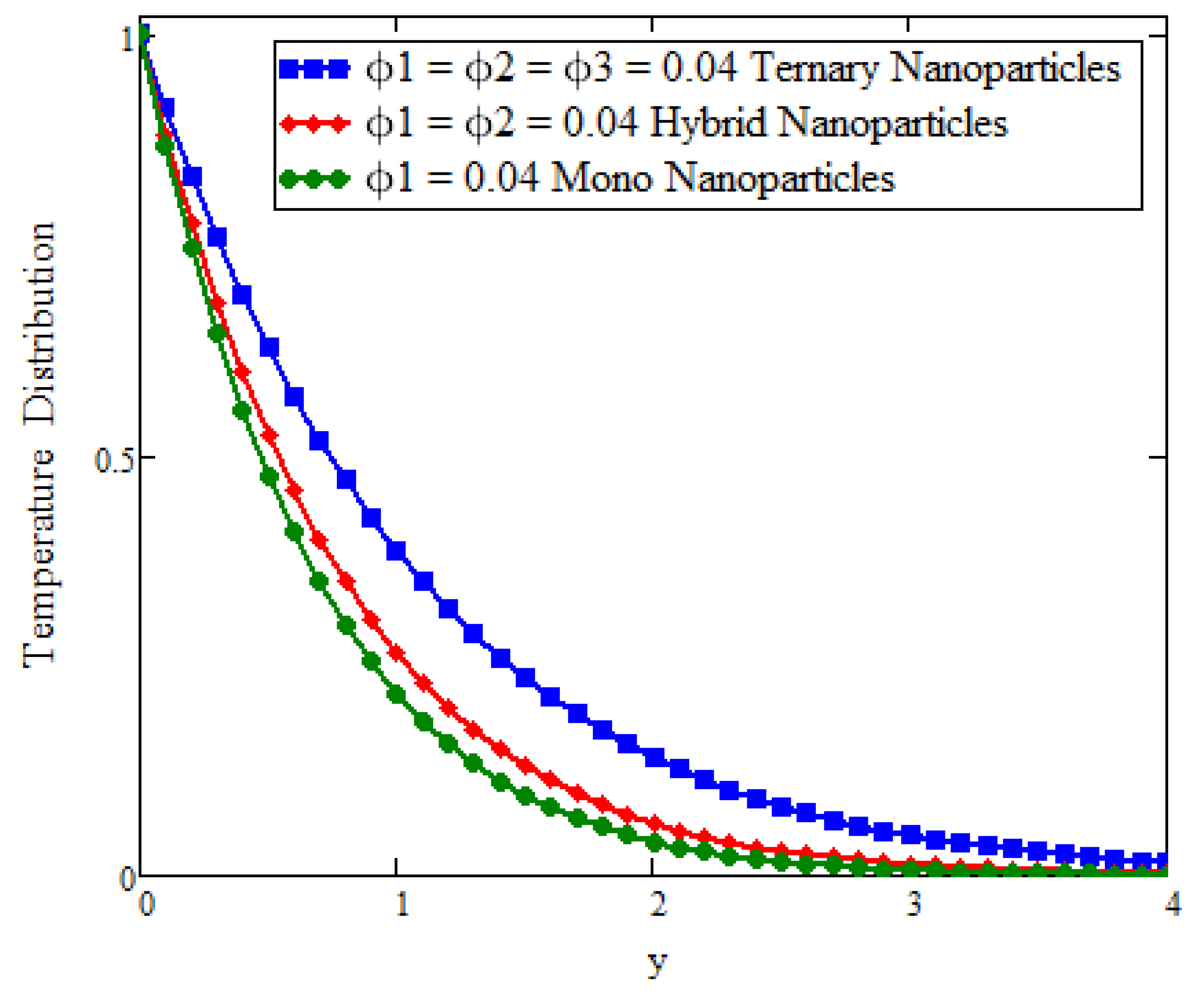
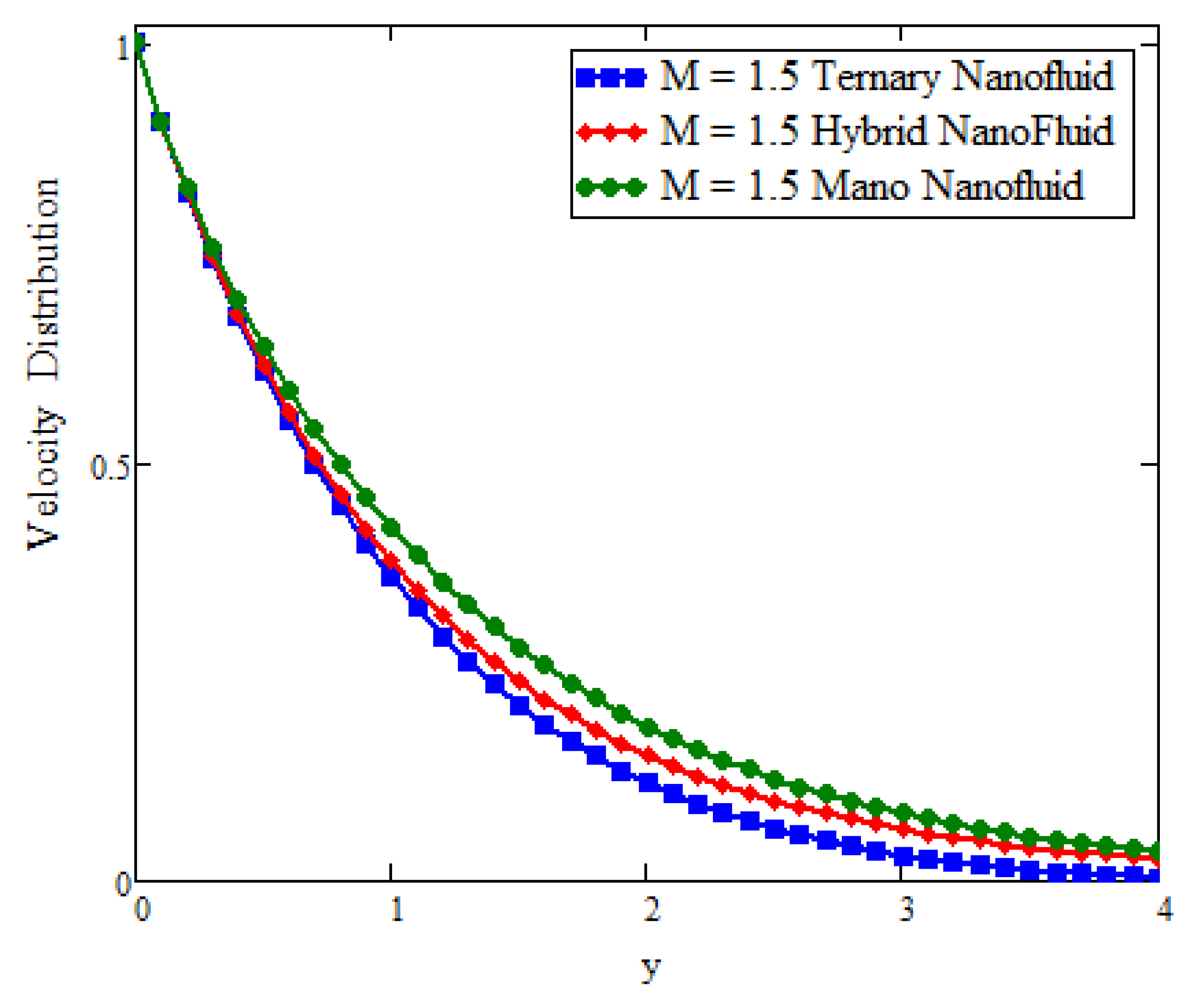
  • The model based on ternary is stronger approach than the hybrid and mono nanoparticle.
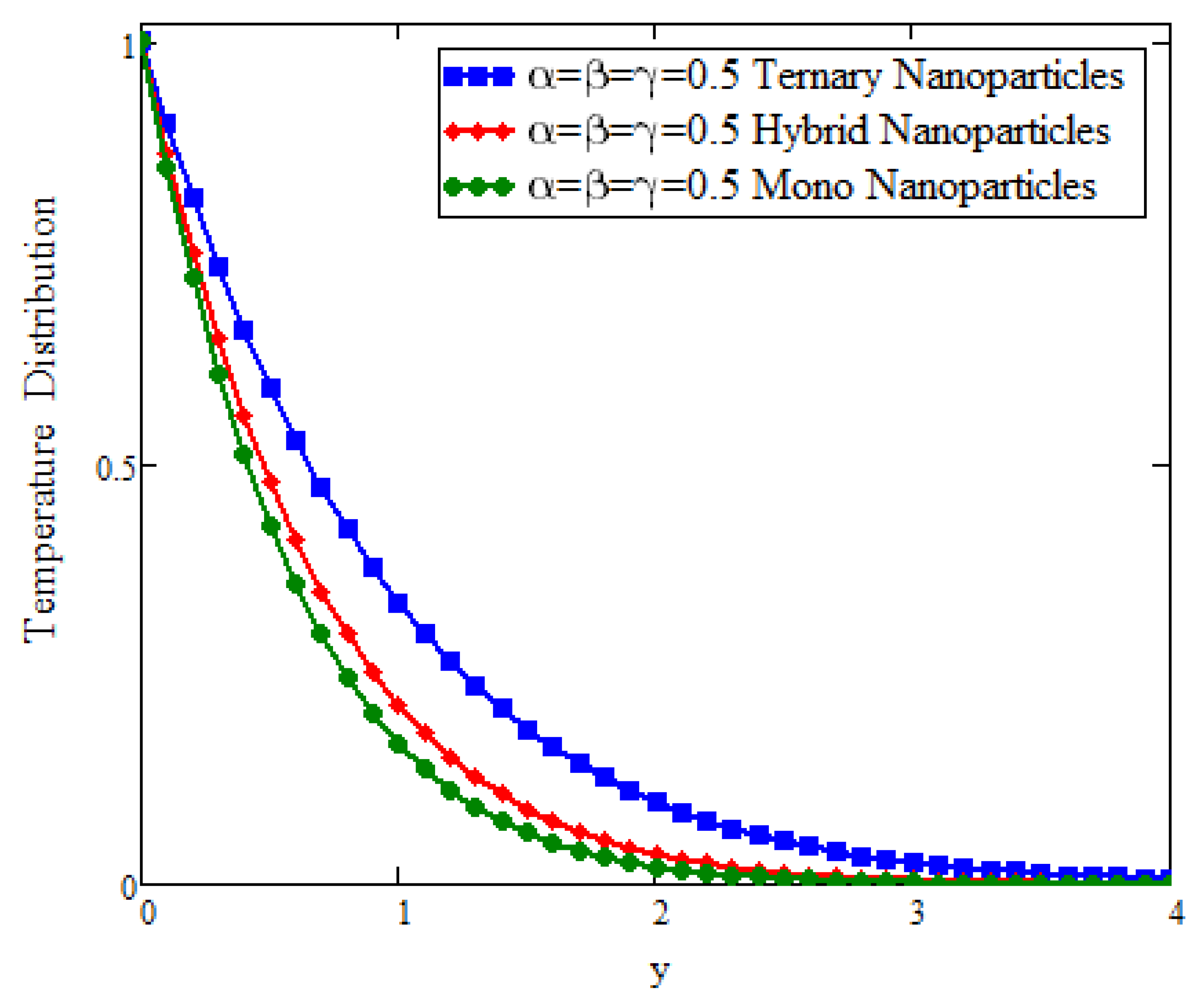
  • Enhancement in temperature and velocity can be achieved for larger values of fractional parameters.
  • Model based on generalized laws are reliable way for fractional modeling and can be accurately fitted any experimental data.
  • Maximum temperature is achievable for ternary nanoparticles instead of hybrid and mono nanoparticles, respectively.

8. Future Work

In the future, this work can be extended for other non-Newtonian fluids, for example, Maxwell; Oldroyd-B; and Micropolar with additional properties such as the heat source and the chemical reaction for different geometries between the two walls of an inclined plane.

Author Contributions

Conceptualization, M.I.A.; methodology, R.K.; validation, A.I.; investigation, M.I.A.; writing—original draft preparation, R.K. and A.H.; writing—review and editing, A.I.; visualization, A.H. and R.K.; supervision, M.I.A.; project administration, S.M.E.; funding acquisition, S.M.E. All authors have read and agreed to the published version of the manuscript.

Funding

This research received no external funding.

Institutional Review Board Statement

Not applicable.

Informed Consent Statement

Not applicable.

Data Availability Statement

All of the data are available inside the research work.

Acknowledgments

The authors are grateful to HEC Pakistan for facilitating this research under research project No. 15911 (NRPU).

Conflicts of Interest

The authors declare no conflict of interest.

Nomenclature

SymbolExplanationUnit
ρ Densitykg/m 3
τ Shear stressPascal (Pa) N/s 2
C p Specific heat capacityJK 1 kg 1
μ Fluid viscositykg/ms
β 0 Casson parameterno unit
Gr Thermal Grashof numberno unit
PrPrandtl numberno unit
Gm Mass Grashof numberno unit
Sc Schimdt numberno unit
gGravitational forcem/s 2
β c Volumetric expansionmol 1 ·m 3
Dmass diffusion coefficientm 3
β T Thermal expansionK 1
α Fractional derivative parameterno unit
β Fractional derivative parameterno unit
γ Fractional derivative parameterno unit
σ Electrical conductivityS·m 1
T Ambient temperatureK
T w Wall temperatureK
C w Wall concentrationmol·m 3
C Ambient concentrationmol·m 3
qFrequency s 1
ν Fluid kinematic viscositym 2 ·s 1
M Dimensionless magnetic parameterno unit
AAccelrationm/s 2

References

  1. Asjad, M.I. Fractional mechanism with power law (singular) and exponential (non-singular) kernels and its applications in bio heat transfer model. Int. J. Heat Technol. 2019, 37, 846–852. [Google Scholar] [CrossRef]
  2. Aleem, M.; Asjad, M.I.; Shaheen, A.; Khan, I. MHD Influence on different water based nanofluids (TiO2, Al2O3, CuO) in porous medium with chemical reaction and newtonian heating. Chaos Solitons Fractals 2020, 130, 109437. [Google Scholar] [CrossRef]
  3. Imran, M.A.; Shah, N.A.; Khan, I.; Aleem, M. Applications of non-integer Caputo time fractional derivatives to natural convection flow subject to arbitrary velocity and Newtonian heating. Neural Comp. Appl. 2018, 30, 1589–1599. [Google Scholar] [CrossRef]
  4. Asjad, M.I.; Shah, N.A.; Aleem, M.; Khan, I. Heat transfer analysis of fractional second-grade fluid subject to Newtonian heating with Caputo and Caputo-Fabrizio fractional derivatives: A comparison. Eur. Physical J. Plus 2017, 132, 1–19. [Google Scholar] [CrossRef]
  5. Tahir, M.; Imran, M.A.; Raza, N.; Abdullah, M.; Aleem, M. Wall slip and non-integer order derivative effects on the heat transfer flow of Maxwell fluid over an oscillating vertical plate with new definition of fractional Caputo-Fabrizio derivatives. Results Phys. 2017, 7, 1887–1898. [Google Scholar] [CrossRef]
  6. Singh, J.; Hristov, J.Y.; Hammouch, Z. (Eds.) New Trends in Fractional Differential Equations with Real-World Applications in Physics; Frontiers Media SA: Lausanne, Switzerland, 2020. [Google Scholar]
  7. Owolabi, K.M.; Atangana, A. Numerical Methods for Fractional Differentiation; Springer: Singapore, 2019; p. 54. [Google Scholar]
  8. Trujillo, J.J.; Scalas, E.; Diethelm, K.; Baleanu, D. Fractional Calculus: Models and Numerical Methods; World Scientific: Singapore, 2016; Volume 5. [Google Scholar]
  9. Hayday, A.A.; Bowlus, D.A.; McGraw, R.A. Free convection from a vertical flat plate with step discontinuities in surface temperature. J. Heat Transfer. 1967, 89, 244–249. [Google Scholar] [CrossRef]
  10. Schetz, J.A. On the approximate solution of viscous-flow problems. J. Appl. Mech. 1963, 30, 263–268. [Google Scholar] [CrossRef]
  11. Malhotra, C.P.; Mahajan, R.L.; Sampath, W.S.; Barth, K.L.; Enzenroth, R.A. Control of temperature uniformity during the manufacture of stable thin-film photovoltaic devices. In Proceedings of the ASME International Mechanical Engineering Congress and Exposition, Anaheim, CA, USA, 13–19 November 2004; Volume 4711, pp. 547–555. [Google Scholar]
  12. McIntosh, R.; Waldram, S. Obtaining more, and better, information from simple ramped temperature screening tests. J. Therm. Anal. Calorim. 2003, 73, 35–52. [Google Scholar] [CrossRef]
  13. Das, S.; Jana, M.; Jana, R.N. Radiation effect on natural convection near a vertical plate embedded in porous medium with ramped wall temperature. Open J. Fluid Dyn. 2011, 1, 1–11. [Google Scholar] [CrossRef] [Green Version]
  14. Nandkeolyar, R.; Das, M.; Sibanda, P. Exact solutions of unsteady MHD free convection in a heat absorbing fluid flow past a flat plate with ramped wall temperature. Bound. Value Probl. 2013, 2013, 1–16. [Google Scholar] [CrossRef]
  15. Seth, G.S.; Hussain, S.M.; Sarkar, S. Hydromagnetic natural convection flow with heat and mass transfer of a chemically reacting and heat absorbing fluid past an accelerated moving vertical plate with ramped temperature and ramped surface concentration through a porous medium. J. Egypt. Math. Soc. 2015, 23, 197–207. [Google Scholar] [CrossRef] [Green Version]
  16. Seth, G.S.; Sharma, R.; Sarkar, S. Natural convection heat and mass transfer flow with Hall current, rotation, radiation and heat absorption past an accelerated moving vertical plate with ramped temperature. J. Appl. Fluid Mech. 2014, 8, 7–20. [Google Scholar]
  17. Seth, G.S.; Sarkar, S.; Hussain, S.M.; Mahato, G.K. Effects of hall current and rotation on hydromagnetic natural convection flow with heat and mass transfer of a heat absorbing fluid past an impulsively moving vertical plate with ramped temperature. J. Appl. Fluid Mech. 2014, 8, 159–171. [Google Scholar]
  18. Seth, G.S.; Ansari, M.S.; Nandkeolyar, R. MHD natural convection flow with radiative heat transfer past an impulsively moving plate with ramped wall temperature. Heat Mass Transf. 2011, 47, 551–561. [Google Scholar] [CrossRef]
  19. Mohd Zin, N.A.; Khan, I.; Shafie, S. Influence of thermal radiation on unsteady MHD free convection flow of Jeffrey fluid over a vertical plate with ramped wall temperature. Math. Probl. Eng. 2016, 2016, 6257071. [Google Scholar] [CrossRef] [Green Version]
  20. Asif, M.; Ul Haq, S.; Islam, S.; Abdullah Alkanhal, T.; Khan, Z.A.; Khan, I.; Nisar, K.S. Unsteady flow of fractional fluid between two parallel walls with arbitrary wall shear stress using Caputo-Fabrizio derivative. Symmetry 2019, 11, 449. [Google Scholar] [CrossRef] [Green Version]
  21. Polito, F.; Tomovski, Z. Some properties of Prabhakar-type fractional calculus operators. arXiv 2015, arXiv:1508.03224. [Google Scholar] [CrossRef]
  22. Elnaqeeb, T.; Shah, N.A.; Mirza, I.A. Natural convection flows of carbon nanotubes nanofluids with Prabhakar-like thermal transport. Math. Methods Appl. Sci. 2020. [Google Scholar] [CrossRef]
  23. Shah, N.A.; Fetecau, C.; Vieru, D. Natural convection flows of Prabhakar-like fractional Maxwell fluids with generalized thermal transport. J. Therm. Anal. Calorim. 2021, 143, 2245–2258. [Google Scholar] [CrossRef]
  24. Eshaghi, S.; Ghaziani, R.K.; Ansari, A. Stability and dynamics of neutral and integro-differential regularized Prabhakar fractional differential systems. Comput. Appl. Math. 2020, 39, 1–21. [Google Scholar] [CrossRef]
  25. Tanveer, M.; Ullah, S.; Shah, N.A. Thermal analysis of free convection flows of viscous carbon nanotubes nanofluids with generalized thermal transport: A Prabhakar fractional model. J. Therm. Anal. Calorim. 2021, 144, 2327–2336. [Google Scholar] [CrossRef]
  26. Alidousti, J. Stability region of fractional differential systems with Prabhakar derivative. J. Appl. Math. Comp. 2020, 62, 135–155. [Google Scholar] [CrossRef]
  27. Derakhshan, M. New numerical algorithm to solve variable—Order fractional integrodifferential equations in the sense of Hilfer Prabhakar derivative. In Abstract and Applied Analysis; Hindawi: London, UK, 2021; Volume 2021. [Google Scholar]
  28. Asjad, M.I.; Sarwar, N.; Hafeez, M.B.; Sumelka, W.; Muhammad, T. Advancement of non-newtonian fluid with hybrid nanoparticles in a convective channel and prabhakars fractional derivative—Analytical solution. Fractal Fract. 2021, 5, 99. [Google Scholar] [CrossRef]
  29. Chen, C.; Rehman, A.U.; Riaz, M.B.; Jarad, F.; Sun, X.E. Impact of Newtonian heating via Fourier and Ficks Laws on thermal transport of oldroyd-B fluid by using generalized Mittag-Leffler kernel. Symmetry 2022, 14, 766. [Google Scholar] [CrossRef]
  30. Wang, F.; Asjad, M.I.; Zahid, M.; Iqbal, A.; Ahmad, H.; Alsulami, M.D. Unsteady thermal transport flow of Casson nanofluids with generalized Mittag-Leffler kernel of Prabhakar’s type. J. Mater. Res. Technol. 2021, 14, 1292–1300. [Google Scholar] [CrossRef]
  31. Sene, N.; Srivastava, G. Generalized Mittag-Leffler input stability of the fractional differential equations. Symmetry 2019, 11, 608. [Google Scholar] [CrossRef] [Green Version]
  32. Nadeem, S.; Ahmad, S.; Khan, M.N. Mixed convection flow of hybrid nanoparticle along a Riga surface with Thomson and Troian slip condition. J. Therm. Anal. Calorim. 2021, 143, 2099–2109. [Google Scholar] [CrossRef]
  33. Reddy, M.G.; Shehzad, S.A. Molybdenum disulfide and magnesium oxide nanoparticle performance on micropolar Cattaneo-Christov heat flux model. Appl. Math. Mech. 2021, 42, 541–552. [Google Scholar] [CrossRef]
  34. Jamei, M.; Pourrajab, R.; Ahmadianfar, I.; Noghrehabadi, A. Accurate prediction of thermal conductivity of ethylene glycol-based hybrid nanofluids using artificial intelligence techniques. Int. Commun. Heat Mass Transf. 2020, 116, 104624. [Google Scholar] [CrossRef]
  35. Xian, H.W.; Sidik, N.A.C.; Saidur, R. Impact of different surfactants and ultrasonication time on the stability and thermophysical properties of hybrid nanofluids. Int. Commun. Heat Mass Transf. 2020, 110, 104389. [Google Scholar] [CrossRef]
  36. Arani, A.A.A.; Aberoumand, H. Stagnation-point flow of Ag-CuO/water hybrid nanofluids over a permeable stretching/shrinking sheet with temporal stability analysis. Powder Technol. 2021, 380, 152–163. [Google Scholar] [CrossRef]
  37. Roy, N.C.; Saha, L.K.; Sheikholeslami, M. Heat transfer of a hybrid nanofluid past a circular cylinder in the presence of thermal radiation and viscous dissipation. AIP Adv. 2020, 10, 095208. [Google Scholar] [CrossRef]
  38. Mousavi, S.M.; Esmaeilzadeh, F.; Wang, X.P. Effects of temperature and particles volume concentration on the thermophysical properties and the rheological behavior of CuO/MgO/TiO2 aqueous ternary hybrid nanofluid. J. Therm. Anal. Calorim. 2019, 137, 879–901. [Google Scholar] [CrossRef]
  39. Sahoo, R.R.; Kumar, V. Development of a new correlation to determine the viscosity of ternary hybrid nanofluid. Int. Commun. Heat Mass Transfer 2020, 111, 104451. [Google Scholar] [CrossRef]
  40. Xia, X.; Chen, Y.; Yan, L. Averaging principle for a class of time-fractal-fractional stochastic differential equations. Fractal Fract. 2022, 6, 558. [Google Scholar] [CrossRef]
  41. Guechi, S.; Dhayal, R.; Debbouche, A.; Malik, M. Analysis and optimal control of ϕ-Hilfer fractional semilinear equations involving nonlocal impulsive conditions. Symmetry 2021, 13, 2084. [Google Scholar] [CrossRef]
  42. Manjunatha, S.; Puneeth, V.; Gireesha, B.J.; Chamkha, A. Theoretical study of convective heat transfer in ternary nanofluid flowing past a stretching sheet. J. Appl. Comput. Mech. 2022, 8, 1279–1286. [Google Scholar]
  43. Nazir, U.; Sohail, M.; Hafeez, M.B.; Krawczuk, M. Significant production of thermal energy in partially ionized hyperbolic tangent material based on ternary hybrid nanomaterials. Energies 2021, 14, 6911. [Google Scholar] [CrossRef]
  44. Nasir, S.; Sirisubtawee, S.; Juntharee, P.; Berrouk, A.S.; Mukhtar, S.; Gul, T. Heat transport study of ternary hybrid nanofluid flow under magnetic dipole together with nonlinear thermal radiation. Appl. Nanosci. 2022, 12, 2777–2788. [Google Scholar] [CrossRef]
  45. Guedri, K.; Bashir, T.; Abbasi, A.; Farooq, W.; Khan, S.U.; Khan, M.I.; Jammel, M.; Galal, A.M. Hall effects and entropy generation applications for peristaltic flow of modified hybrid nanofluid with electroosmosis phenomenon. J. Indian Chem. Soc. 2022, 99, 100614. [Google Scholar] [CrossRef]
  46. Saqib, M.; Mohd Kasim, A.R.; Mohammad, N.F.; Chuan Ching, D.L.; Shafie, S. Application of fractional derivative without singular and local kernel to enhanced heat transfer in CNTs nanofluid over an inclined plate. Symmetry 2020, 1, 768. [Google Scholar] [CrossRef]
  47. Irandoost Shahrestani, M.; Maleki, A.; Safdari Shadloo, M.; Tlili, I. Numerical investigation of forced convective heat transfer and performance evaluation criterion of Al2O3/water nanofluid flow inside an axisymmetric microchannel. Symmetry 2020, 12, 120. [Google Scholar] [CrossRef] [Green Version]
  48. Kumar, M.A.; Reddy, Y.D.; Rao, V.S.; Goud, B.S. Thermal radiation impact on MHD heat transfer natural convective nano fluid flow over an impulsively started vertical plate. Case Stud. Therm. Eng. 2021, 24, 100826. [Google Scholar] [CrossRef]
  49. Reyaz, R.; Mohamad, A.Q.; Lim, Y.J.; Saqib, M.; Shafie, S. Analytical solution for impact of Caputo-Fabrizio fractional derivative on MHD casson fluid with thermal radiation and chemical reaction effects. Fractal Fract. 2022, 6, 38. [Google Scholar] [CrossRef]
  50. Sarwar, N.; Jahangir, S.; Asjad, M.I.; Eldin, S.M. Application of Ternary Nanoparticles in the Heat Transfer of an MHD Non-Newtonian Fluid Flow. Micromachines 2022, 13, 2149. [Google Scholar] [CrossRef]
  51. Sarwar, N.; Asjad, M.A.; Sitthiwirattham, T.; Patanarapeelert, N.; Muhammad, T. A Prabhakar fractional approach for the convection flow of casson fluid across an oscillating surface based on the generalized Fourier law. Symmetry 2021, 13, 2039. [Google Scholar] [CrossRef]
  52. Maiti, S.; Shaw, S.; Shit, G.C. Caputo-Fabrizio fractional order model on MHD blood flow with heat and mass transfer through a porous vessel in the presence of thermal radiation. Phys. A Stat. Mech. Its Appl. 2020, 540, 123149. [Google Scholar] [CrossRef]
  53. Hussanan, A.; Zuki Salleh, M.; Tahar, R.M.; Khan, I. Unsteady boundary layer flow and heat transfer of a Casson fluid past an oscillating vertical plate with Newtonian heating. PLoS ONE 2014, 9, e108763. [Google Scholar] [CrossRef]
Figure 1. Physical model of the problem [49].
Processes 11 00218 g001
Figure 2. Comparison of temperature assessment across y as α = 0.5 , β = 0.5 , and γ = 0.5 when t = 0.04, Sc = 1.5 , and Pr = 21 .
Processes 11 00218 g002
Figure 3. Comparison of temperature assessment across y as volume fraction ϕ 1 = ϕ 2 = ϕ 3 = 0.01 when α = β = γ = 0.5 , t = 0.04, Sc = 1.5 , and Pr = 21 .
Processes 11 00218 g003
Figure 4. Comparison of temperature assessment with Pr across y as α = 0.5 , β = 0.5 , and γ = 0.5 when t = 0.04 and Sc = 1.5 .
Processes 11 00218 g004
Figure 5. Comparison of velocity assessment with α β γ across y as Sc = 9.2 when t = 1, α = β = γ = 0.2 , M = 1.5 , and Pr = 21 .
Processes 11 00218 g005
Figure 6. Comparison of velocity assessment with Gm across y as α = β = γ = 0.5 when t = 1, Sc = 9.2 , ϕ 1 = 0.02 , ϕ 2 = 0.03 , ϕ 3 = 0.04 , Pr = 21 , and M = 1.5 .
Processes 11 00218 g006
Figure 7. Comparison of velocity assessment with Gr across y as α = 0.5 , β = 0.5 , γ = 0.5 when t = 1, Sc = 9.2 , ϕ 1 = 0.02 , ϕ 2 = 0.03 , ϕ 3 = 0.04 , Pr = 21 , and M = 1.5 .
Processes 11 00218 g007
Figure 8. Comparison of velocity assessment with volume fraction across y as α = β = γ = 0.5 when t = 1, Pr = 21 , and M = 1.5 .
Processes 11 00218 g008
Figure 9. Comparison of velocity assessment with magnetic parameter M across y as α = 0.3 , β = 0.3 , γ = 0.3 when t = 1, ϕ 1 = 0.03 , ϕ 2 = 0.03 , ϕ 3 = 0.03 , Pr = 21 , Gm = 1.4 , and Gr = 1.5 .
Processes 11 00218 g009
Table 1. Thermophysical possessions of nanoparticles and base fluid [48].
MaterialBase Fluid Kerosene OilSilver (Ag)Copper (Cu)Titanium Dioxide (TiO 2 )
ρ (kg /m 3 )86310,50089934250
C p (J/kg.K)2048235385686.20
k (W/m.K)0.14044294018.9538
σ (s/m) 55 × 10 6 3.6 × 10 7 5.96 × 10 7 1 × 10 12
β × 10 5 (1/K)701.891.670.90
Disclaimer/Publisher’s Note: The statements, opinions and data contained in all publications are solely those of the individual author(s) and contributor(s) and not of MDPI and/or the editor(s). MDPI and/or the editor(s) disclaim responsibility for any injury to people or property resulting from any ideas, methods, instructions or products referred to in the content.

