Process Model Inversion in the Data-Driven Engineering Context for Improved Parameter Sensitivities ^†

Abstract

Industry 4.0 has embraced process models in recent years, and the use of model-based digital twins has become even more critical in process systems engineering, monitoring, and control. However, the reliability of these models depends on the model parameters available. The accuracy of the estimated parameters is, in turn, determined by the amount and quality of the measurement data and the algorithm used for parameter identification. For the definition of the parameter identification problem, the ordinary least squares framework is still state-of-the-art in the literature, and better parameter estimates are only possible with additional data. In this work, we present an alternative strategy to identify model parameters by incorporating differential flatness for model inversion and neural ordinary differential equations for surrogate modeling. The novel concept results in an input-least-squares-based parameter identification problem with significant parameter sensitivity changes. To study these sensitivity effects, we use a classic one-dimensional diffusion-type problem, i.e., an omnipresent equation in process systems engineering and transport phenomena. As shown, the proposed concept ensures higher parameter sensitivities for two relevant scenarios. Based on the results derived, we also discuss general implications for data-driven engineering concepts used to identify process model parameters in the recent literature.

1. Introduction

In process systems engineering (PSE), using a mathematical model allows prediction and analysis of the characteristics, design, and optimal operating conditions of the process under study, thus contributing to Industry 4.0 and process digitization [1,2,3,4]. However, before a mathematical model can be implemented, decisions must be made about the modeling strategy. For example, knowledge-based first-principles models (white-box models) allow extrapolation beyond the range of data available and, consequently, are highly relevant for process analysis and system understanding [5]. Data-driven models (black-box models), in turn, are interpolative in nature, with less insight into cause-effect relationships. There are also the so-called hybrid models (gray-box models), which combine partial process knowledge with data-driven surrogates that are constructed using experimental data [5,6,7,8,9,10]. However, the use of surrogate models introduces new difficulties, e.g., improper definitions of the surrogate model or biased training procedures, as well as their lack of interpretability and explainability [11,12,13,14]. In addition to these individual advantages and disadvantages, all of the modeling approaches mentioned also have fundamental common challenges in terms of system identification, including the need for experimental data and parameter estimation, model validation, and model refinement, as well as numerical implementation aspects [5]. In PSE, the dynamic process behavior is of utmost interest and is typically described with ordinary differential equations (ODEs) or partial differential equations (PDEs). However, the parameters of these first-principles models are often unknown and must be estimated with a limited amount of noisy experimental data [15,16,17]. In many parameter optimization routines, see [18] and references therein, for the loss term, the sum of squared errors (SSE) is used to measure the difference between the response of the model and the measured data [18], resulting in an ordinary least squares (OLS) framework.

In engineering and science, uncertainties must be integrated for any meaningful model prediction, including variations in the estimates of the derived model parameters. Especially for OLS, it is well known that with parameter sensitivities and the inverse of the so-called Fisher information matrix, parameter uncertainties can be inferred as statistical measures, i.e., variances, correlations, and confidence regions, respectively [11,18]. In addition to parameter sensitivity studies and uncertainty quantification, if necessary, model-based optimal experimental design (MBDoE) concepts can be applied to efficiently improve the quantity and quality of experimental data, resulting in more precise parameter estimates [19,20,21]. Note that MBDoE, in the case of non-linear parameter identification problems, which are standard in PSE, may result in suboptimal experimental designs [22]. The same is true for hybrid models, where changes in parameter sensitivities are reported that cannot be directly compared with their counterparts in first-principles models [23]. In addition to the problem-dependent shortcomings mentioned, MBDoE has a general weakness; i.e., the need for additional experimental data, which is typically a considerable investment in time and cost [19].

Alternatively, online MBDoE methods (e.g., based on Kalman Filtering [19,24]) try to adjust experimental conditions in real-time and to improve model parameter estimates during the experimental run. Moreover, instead of aiming for additional data at all, there are strategies that focus entirely on revising the parameter identification problem definition. For example, a so-called extent-based approach is proposed to identify the model parameters that result in more precise parameter estimates and smaller confidence intervals [25], respectively. Also, the iteratively refined principal differential analysis (iPDA) approach defines the parameter identification problem differently. It involves fitting B-splines to the measured data, from which time-derivative information can be obtained to define a loss function solely on the ODE system of the process model. Thus, unlike the standard OLS setting, the ODEs of the process model do not need to be solved numerically [26,27]. Advanced model inversion schemes, similarly, result in total least squares (TLS) loss functions while recalculating the model inputs, i.e., the OLS framework is extended with an input least squares (ILS) expression [28,29]. It is also based on the concept of differential flatness originally introduced in control and systems theory [30]. In particular, so-called flat outputs are obtained by fitting measurement data with empirical functions (e.g., B-splines), and the inverse process model is derived subsequently for TLS-based parameter estimates [29,31,32]. In data-driven engineering, instead, physics-informed neural networks (PINNs) were first designed to replace numerical ODE/PDE solvers [33,34], but the recent literature also shows promising PINN-based results in system identification and model parameter estimates [35,36,37,38]. An equally successful technique in the field of data-driven engineering, are so-called neural ODEs (nODEs) as a deep learning approach for empirical process modeling [39,40]. With nODEs, it is possible to create surrogate models, i.e., black-box dynamics, and ensure system identification of dynamic processes even with sparse and noisy data [41,42,43,44].

While reliable parameter estimate results, particularly for PINN, are reported in the literature [37,38], a closer look at changes in parameter sensitivities in terms of loss functions applied is missing. As mentioned, parameter sensitivities, in turn, have a significant impact on the derived parameter precision and thus, are of fundamental interest. To the best of the authors’ knowledge, this is the first work using a model inversion concept based on differential flatness in combination with nODEs studying changes in model parameter sensitivities in ILS-based parameter identification problems. Note that the proposed concept also helps to dissect particular PINN-oriented parameter identification problems in terms of parameter sensitivities and to explain improved parameter estimate outcomes theoretically.

To this end, in this work, which is an extended version of our Electronic Conference on Processes: Processes System Innovation (ECP) 2022 contribution [45], the differential flatness concept and neural ordinary differential equations are explained in Section 2. The dynamics of the diffusion model and the two assumed control scenarios, that is, the distributed control problem and the boundary control, are discussed in Section 3. The simulation results that include some discussion on the advantages of adapting the flatness concept and the findings of the sensitivity analyzes are presented in Section 4. Finally, we provide some concluding remarks in Section 5.

2. Problem Formulation

The standard iterative workflow used for system identification is shown in Figure 1. The first requirement for determining any process model is the collection of data (or measurements) from the process under study. Next, a model candidate is postulated or selected from a set of model candidates. Then, for the chosen model candidate, the corresponding model parameters are identified. The model with the estimated model parameters is validated in terms of residuals, parameter uncertainties, and model complexity. If the criteria for this precision are not satisfied, an optimized experimental protocol is implemented, i.e., following a model-based Design of Experiment (MBDoE) strategy. Consequently, additional experimental data are gathered, and the parameter identification and uncertainty quantification steps are repeated [18,19].

As mentioned, the fundamental question is to what extent parameter sensitivities and estimation accuracies can be improved without additional data by using systems theory methods with data-driven engineering concepts. The required methods to tackle this open problem are explained in more detail below.

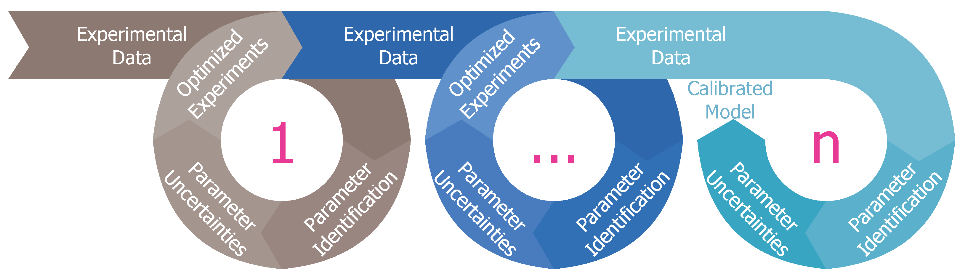
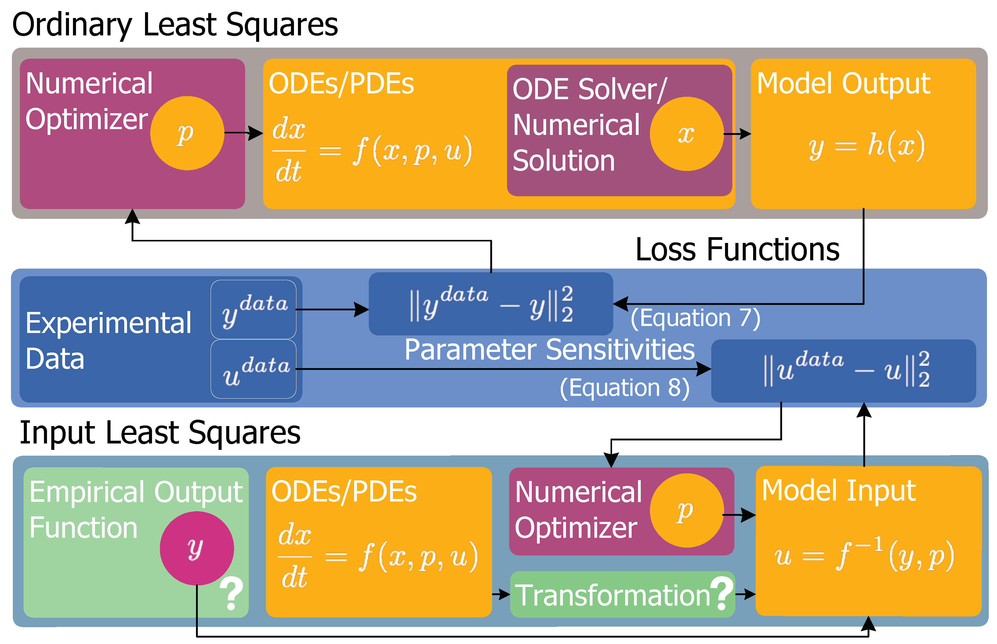
2.1. Parameter Identification Strategies

For the sake of simplicity but without loss of generality, the proposed concept is demonstrated with a common PDE problem. To this end, the parabolic equation for diffusion problems and the unknown $\mathrm{\Phi }(\mathbf{x},\mathbf{y},\mathbf{z},t)$ with $\mathbf{x},\mathbf{y},\mathbf{z}$ and t for space and time, respectively, over a bounded domain $\mathrm{\Omega }$ and a finite time interval $0\le t\le T$ are studied and represented by the following expression [46]:

$$\left\{\begin{array}{c}\frac{\partial \mathrm{\Phi }}{\partial t}-\kappa \mathsf{\Delta }\mathrm{\Phi }=u\mathrm{in}\mathrm{\Omega }\times (0,T]\hfill \\ \mathrm{\Phi }(\mathbf{x},0)={\mathrm{\Phi }}_0\left(\mathbf{x}\right)\mathrm{in}\mathrm{\Omega },\mathrm{for}t=0\hfill \\ \mathrm{boundary}\mathrm{conditions}\mathrm{on}\partial \mathrm{\Omega }\hfill \end{array}\right.$$

(1)

where $\mathsf{\Delta }\doteq {\partial }^2/\partial {\mathbf{x}}^2+{\partial }^2/\partial {\mathbf{y}}^2+{\partial }^2/\partial {\mathbf{z}}^2$ and $\partial \mathrm{\Omega }$ is the boundary of $\mathrm{\Omega }$, $\kappa$ is an unknown time-invariant parameter, u is some known function (e.g., the system control affine input).

When simulating a PDE model, all the involved parameters (coefficients or source terms) are assumed to be known, and for this, these parameters have to be determined. They are often hardly accessible to direct measurements, leading to the need for indirect measurements, which amounts to a parameter identification problem. However, there are two types of problems, namely well-posed and ill-posed problems. The former always has a unique solution and depends on the given data, while the latter requires tedious efforts for precise parameter estimates. Furthermore, when using techniques such as the Method of Lines (MOL) [47,48,49] to solve the PDE system numerically, the resulting discretized system along, for instance, the axis $\mathbf{x}$ at points ${\mathbf{x}}_0+i\mathsf{\Delta }\mathbf{x}$, $i=1,2,\cdots ,N$ reads as [31]:

$$\begin{array}{c}\hfill \frac{\partial {\mathrm{\Phi }}_i}{\partial t}=\frac{\kappa }{\mathsf{\Delta }{\mathbf{x}}^2}{\mathrm{\Phi }}_{i+1}-\frac{2\kappa }{\mathsf{\Delta }{\mathbf{x}}^2}{\mathrm{\Phi }}_i+\frac{\kappa }{\mathsf{\Delta }{\mathbf{x}}^2}{\mathrm{\Phi }}_{i-1}+u.\end{array}$$

(2)

Consequently, these PDEs are approximated by an ODE system with the state vector $x^{\top }=({\mathrm{\Phi }}_1,{\mathrm{\Phi }}_2,\cdots ,{\mathrm{\Phi }}_N)$ according to:

$$\begin{array}{c}\hfill \left\{\begin{array}{c}\dot{x}\left(t\right)=f(x\left(t\right),u\left(t\right),p),\hfill \\ x\left(t_0\right)=x_0,\hfill \end{array}\right.\end{array}$$

(3)

where $t\in [t_0,t_{end}]$, with $t_0$ as the initial time and $t_{end}$ as the time duration of the simulation, $u\in {\mathbf{R}}^{n_u}$ is the vector of the control variables, $p\in {\mathbf{R}}^{n_p}$ is the unknown time-invariant parameter, and $x\in {\mathbf{R}}^{n_x}$ are the system states. The initial conditions for the differential states are given by $x_0$. Moreover, $f:{\mathbf{R}}^{n_x\times n_u\times n_p}\to {\mathbf{R}}^{n_x}$ represents the corresponding vector field. For this kind of mathematical representation, the standard approach of parameter identification, i.e., the OLS-based method, following the notation given in [18], can be defined as:

$$\begin{array}{c}\hfill {\widehat{p}}^{OLS}=arg\underset{p}{min}\sum _{k=1}^K{\parallel y^{data}\left(t_k\right)-y(t_k,p)\parallel }_2^2,\end{array}$$

(4)

where ${\parallel .\parallel }_2$ denotes the Euclidean norm, $y^{data}\left(t_k\right)$ represents the data vector at discrete time points $t_k$ over all measurement samples K, and the output function of the model is defined as follows:

$$\begin{array}{c}\hfill y(t_k,p)=h\left(x(t_k,p)\right),\end{array}$$

(5)

with $h:{\mathbf{R}}^{n_x}\to {\mathbf{R}}^{n_y}$ and $y\in {\mathbf{R}}^{n_y}$ as the output function and the model output, respectively. Alternatively, when aiming to utilize the inverse model response [18], that is, applying a model inversion strategy, an ILS-based parameter identification problem can be used:

$$\begin{array}{c}\hfill {\widehat{p}}^{ILS}=arg\underset{p}{min}\sum _{k=1}^K{\parallel u^{data}\left(t_k\right)-u(t_k,p)\parallel }_2^2,\end{array}$$

(6)

Here, the control inputs, $u(t_k,p)$, have to be calculated to solve the parameter identification problem, and $u^{data}\left(t_k\right)$ represents the physical input actions recorded. For this purpose, in this work, we study the differential flatness concept as outlined in Section 2.2. However, it is essential to note that parameter sensitivities are relevant for well-posed parameter identification problems. When having the output function $y(t_k,p)$ and the inputs $u(t_k,p)$ (inverse model response), the sensitivity S of the parameter p, in accordance to [50], as follows:

$$\begin{array}{c}\hfill S_{y_p}\left(t_k\right)=\frac{\partial y(t_k,p)}{\partial p},\end{array}$$

(7)

$$\begin{array}{c}\hfill S_{u_p}\left(t_k\right)=\frac{\partial u(t_k,p)}{\partial p}.\end{array}$$

(8)

Note, as mentioned previously, high parameter sensitivity values are expected to ensure precise parameter estimates according to the Fisher information matrix and the Cramér Rao inequality [18,19].

In this study, a generic one-dimensional diffusion-type problem is considered, i.e., an omnipresent equation in process systems engineering and transport phenomena. The parameter identification results for the model under study are derived by the following steps: (i) rearrangement of the model equations to solve for the model input, where these equations contain the model’s flat outputs and their derivatives with respect to time, (ii) the outputs and their derivatives are obtained from a neural ODE that was trained on a given data set, (iii) minimization of the SSE between the predicted model and the data, referred to as ordinary least squares (OLS), (iv) minimization of the SSE between prediction and input values, referred to as input least squares (ILS), and (v) the estimated parameters are compared for precision using the results of the sensitivity analysis.

The OLS and the ILS framework are summarized in Figure 2. As described previously, OLS follows the classical forward simulation of the underlying process model (Equation (3)) strategy and thus needs numerical ODE solvers to derive the output function $h(·)$ for loss term evaluation, i.e., differences between measurements and the output function, and model parameter p adaptation (Equation (4)). Note that for the parameter p adaptation itself numerical optimization routines have to be used as well. Basically, these steps of forward simulation, loss function evaluation, and model parameter adaptation are reiterated until a good model-data fit is achieved. For the ILS setting, in turn, we see that the numerical solution of the underlying process model is replaced with a transformation step aiming to recalculate the corresponding model input. As the expressed model input, in turn, is still based on the process model, it depends on the model parameter p, too. On that note, the model input is used to define an input-based loss function followed again by a model parameter adaptation step (Equation (6)) realized with a numerical optimization routine. Both iterative parameter identification procedures might behave differently for parameter sensitivities and result in different parameter estimates and parameter uncertainties, respectively. The change in parameter sensitivities, however, is difficult to predict and thus a central element of this work. Moreover, in the case of ILS, the mandatory transformation step to calculate the model input, as well as the mathematical representation of the model output (i.e., empirical output function) needed for this particular transformation step, are the other two major contributions of this work and are discussed in detail in the following subsections.

2.2. Transformation: Differential Flatness

The model inputs $u(t_k,p)$ in Equation (6) are determined using this concept of model inversion. In the literature, a process model (Equation (3)) is called differentially flat if there exists an output function [30]:

$$\begin{array}{c}\hfill y^{flat}=h^{flat}(x,u,\dot{u},\cdots ,u^{\left(s\right)},p),\end{array}$$

(9)

with a finite value $S\in N$ and the smooth mapping function $y^{flat}:{\mathbf{R}}^{n_x}\times {\left({\mathbf{R}}^{n_u}\right)}^{s+1}\times {\mathbf{R}}^{n_p}\to {\mathbf{R}}^{n_y}$ that is called a flat output. With the flat output, the system states and control inputs are expressed as [30]:

$$\begin{array}{c}\hfill x={\mathrm{\Psi }}_x(y^{flat},{\dot{y}}^{flat},\cdots ,y^{fla{t}^{\left(r\right)}},p),\end{array}$$

(10)

$$\begin{array}{c}\hfill u={\mathrm{\Psi }}_u(y^{flat},{\dot{y}}^{flat},\cdots ,y^{fla{t}^{(r+1)}},p),\end{array}$$

(11)

with the mapping functions ${\mathrm{\Psi }}_x:{\left({\mathbf{R}}^{n_y}\right)}^{r+1}\times {\mathbf{R}}^{n_p}\to {\mathbf{R}}^{n_x}$ and ${\mathrm{\Psi }}_u:{\left({\mathbf{R}}^{n_y}\right)}^{r+2}\times {\mathbf{R}}^{n_p}\to {\mathbf{R}}^{n_u}$, and assuming a quadratic system $dim{y}^{flat}=dimu$. When applying the flatness concept, it was shown that parameter sensitivities and reliability of parameter estimates, respectively, could be improved in the case of ILS [28], or when OLS was combined with ILS [29,32]. However, in process systems engineering, for instance, in addition to lumped-parameter systems (i.e., ordinary differential equations) [51], distributed-parameter systems described via partial differential equations are frequently applied. In this case, the differential flatness approach must be generalized [31,52,53,54].

A model-based approach can also be described for a boundary control problem assuming a linear diffusion-convection reaction system. Here, by exploiting the flatness property of the PDE, the optimal control problem could be formulated in terms of the flat output and its higher time derivatives, imposed by an integrator chain [55]. The method uses an observer to estimate the states of the integrator chain from the PDE solution. Different combinations of flatness and MPC control are proposed in the ODE case, which relies on expressing the flat output as a sum of weighted, linearly independent functions, which are then used as decision variables when formulating the optimal control problem as a state optimization problem. The use of an integrator chain to determine a reference trajectory and its derivatives for flat output is shown in [56]. Different extensions of the flatness concept are available for PDE systems that rely on the Laplace transform, formal power series, spectral analysis, and formal integration [54].

This work exploits the flatness property of the system’s flat output to solve distributed and boundary control problems to perform the model inversion. The importance of boundary control for distributed parameter systems described by non-linear PDEs and its elevated difficulty are discussed for several applications [57,58,59]. When model inversion is achieved, it initiates a possible use of the determined control input in parameter identification. Sensitivity values provide useful information on how a variable could improve the precision of parameter estimates within the framework of the Fisher information matrix based on local parameter sensitivities and the Cramér Rao inequality [18].

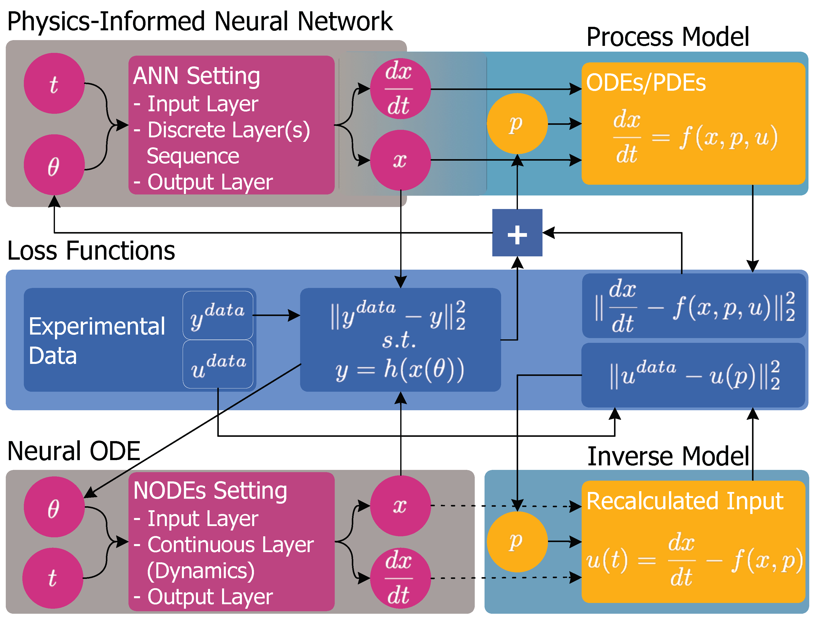
2.3. Empirical Output Function: Neural Ordinary Differential Equations

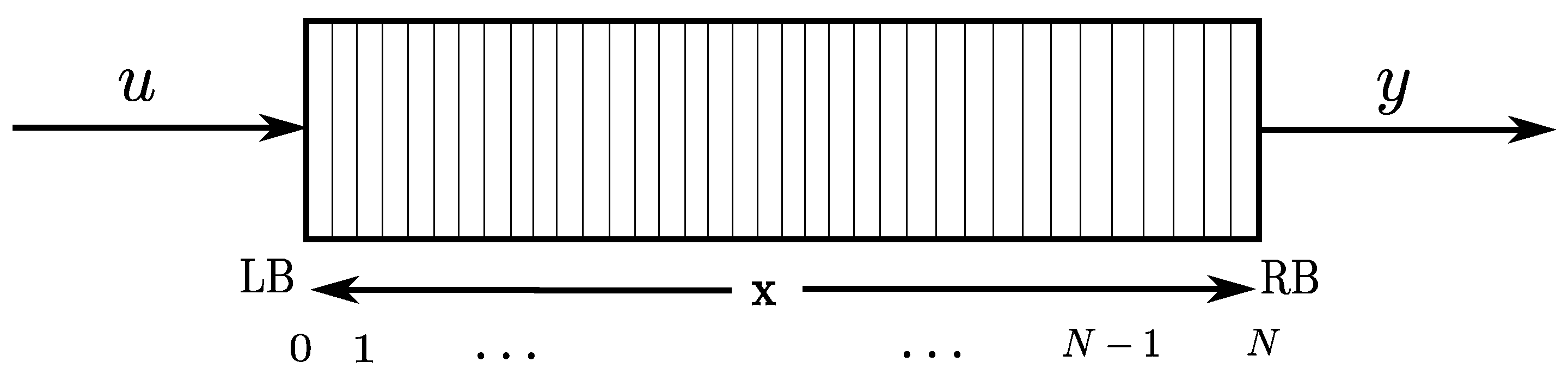
In data engineering, neural networks are often used to create surrogate models. The first and last layers of a typical multilayer feedforward neural network are termed input and output layers, respectively. Various hidden layers can be interposed, conducting the transformation of the input to the output prediction according to the specific input-output behavior of the process under study. This transformation is governed by the weights and biases of the hidden layers. These are the trainable hyperparameters of the neural network. The activation of a single unit in a hidden layer, a neuron, is defined by the connections with the neurons from the previous layer. This consists of a weighting factor and a threshold set by the neuron-specific bias. In detail, the $j^{th}$ neural network layer, $NN{L}_j\left(\widehat{x}\right):{\mathbf{R}}^{d_{j-1}}\to {\mathbf{R}}^{d_j}$, is specified with the weight matrix, $W^j\in {\mathbf{R}}^{d_j\times d_{j-1}}$, and the bias vector, $b_j\in {\mathbf{R}}^{d_j}$. Thus, for instance, a feedforward neural network reads:

$$\begin{array}{ccc}\hfill NN{L}_0\left(\widehat{x}\right)& =& \widehat{x}\in {\mathbf{R}}^{d_0},\hfill \\ \hfill NN{L}_j\left(\widehat{x}\right)& =& \sigma (W^{j}NN{L}_{j-1}\left(\widehat{x}\right)+b_j)\in {\mathbf{R}}^{d_j},\forall 1\le j\le I-1,\hfill \\ \hfill NN{L}_I\left(\widehat{x}\right)& =& W^{I}NN{L}_{I-1}\left(\widehat{x}\right)+b_I\in {\mathbf{R}}^{d_I},\hfill \end{array}$$

(12)

with the input layer ${\mathrm{NNL}}_0$, the hidden layer ${\mathrm{NNL}}_j$, and the output layer ${\mathrm{NNL}}_I$. The activation function $\sigma (·)$ introduces non-linearity into the input-output-transformation [60].

Concerning the so-called neural ordinary differential equations, the system output is not predicted directly by the neural network, but its derivatives with respect to the independent variable in the ODE system, usually time. According to [39,40,41], this data-driven dynamical systems representation can be expressed as follows:

$$\begin{array}{c}\hfill \dot{\widehat{x}}\left(t\right)=NN(\widehat{x}\left(t\right),u\left(t\right),\theta ),\widehat{x}\left(t_0\right)={\widehat{x}}_0,\end{array}$$

(13)

where the $\widehat{x}$ notation already indicates that Equation (13) is used to approximate the system states, and $\theta$ comprises all ANN hyperparameters. Then, an ODE solver is used to translate the nODE system into the trajectory of the respective system output, $\widehat{y}$. Since this step enables the user to obtain the solution at any (time) point in the observation window according to the specifications in the solver settings [61], a neural ODE resembles the powerful residual networks [62], and thus provides a promising approach to hybrid modeling and system identification [10,63,64,65]. Furthermore, the neural network architecture can be optimized to represent the experimental data better. This could be done in conjunction with optimal experimental design methods [19] to improve the accuracy of system identification or by adding additional input and output layers [36].

Note that when using the PINN approach to solve ODEs/PDEs and to estimate model parameters, the corresponding cost function also has at least two terms:

$$\mathcal{L}(\theta ,p)={\mathcal{L}}^{\mathrm{data}}\left(\theta \right)+{\mathcal{L}}^{\mathrm{ode}}(\theta ,p),$$

(14)

with ${\mathcal{L}}^{\mathrm{data}}$ defined for the measured states $y^{data}$:

$${\mathcal{L}}^{\mathrm{data}}\left(\theta \right)=\sum _{k=1}^K{\parallel y^{data}\left(t_k\right)-\widehat{y}(t_k,\theta )\parallel }_2^2,$$

(15)

and ${\mathcal{L}}^{\mathrm{ode}}$ relates to the governing equation as:

$${\mathcal{L}}^{\mathrm{ode}}(\theta ,p)=\sum _{l=1}^{n_x}\left[\sum _{n=1}^{N^{\mathrm{ode}}}{\left({\left.\frac{d{\widehat{x}}_l}{dt}\right|}_{{\tau }_n}-f_l\left({\widehat{x}}_l\left({\tau }_n,\theta \right),p\right)-u_l\left({\tau }_n\right)\right)}^2\right].$$

(16)

First, an ANN has to fulfill the governing equation system, and second, the ANN has to fit experimental data alike. Interestingly, when we assume that all system states are measurable, solving the PINN problem has much in common with model inversion. Technically, the PINN-based parameter identification problem follows a total least squares (TLS) philosophy, i.e., the combination of OLS (e.g., fitting the data) and ILS (e.g., fulfilling the equation system). The proposed concept of combining model inversion with nODEs, in turn, where these two steps are solved sequentially, helps explain the observed phenomenon of improved parameter estimates for PINN-based parameter identification problems. Both concepts, PINN and the nODE with the inverse model, are summarized and compared in Figure 3. Please note that for the sake of readability, the distinction between the approximated system states $\widehat{x}$ for ANN/nODE-based predictions and the predictions of the process model x is omitted, and the correct solution x is used exclusively. As also indicated in Figure 3, in case of a control affine input problem:

$$\frac{dx}{dt}=f(x,p)+u\left(t\right),$$

(17)

with zero input, $u^{data}\stackrel{!}{=}0$, and assuming that all system states are measurable, $y=h\left(x\right)\stackrel{!}{=}x$, the two loss terms, i.e., for the model input differences (Equation (6)) in ILS and ${\mathcal{L}}^{\mathrm{ode}}$ (Equation (16)) for the PINN-based approach become equivalent:

$${\parallel u}^{data}-u\left(p\right){\parallel }_2^2=\parallel u\left(p\right){\parallel }_2^2\stackrel{!}{=}\parallel \frac{dx}{dt}-f(x,p){\parallel }_2^2.$$

(18)

To the best of the authors’ knowledge, this is the first study addressing the change in parameter sensitivity from this point of view. In addition, for the two concepts, it becomes clear that the adjustment of the model parameter p itself follows an iterative cycle in which the corresponding loss functions are evaluated; however, the type of loss function definitions and their processing differ. Moreover, the strategy to train the related neural network realizations while adjusting their hyperparameters $\theta$ is inherently distinct.

3. Case Study

Determining the kinetic parameters of diffusion-type parabolic PDEs (see Equation (19)) has been extensively studied, including chromatography and adsorption processes [24,66,67,68,69], respectively.

$$\begin{array}{c}\hfill \frac{\partial \mathrm{\Phi }}{\partial t}=\kappa \frac{{\partial }^2\mathrm{\Phi }}{\partial {\mathbf{x}}^2}+u(\mathbf{x},t),\end{array}$$

(19)

where $\mathrm{\Phi }$ is the diffusing state, $\kappa$ is the diffusion coefficient, u is the system input, x is the spatial variable and t is time. Aiming for a numerical solution making use of the finite difference method (Equation (20)) of the diffusion-type PDE problem, an ODE system is obtained, which can be written in a state space form [31] as shown in Equation (21).

$$\frac{{\partial }^2\mathrm{\Phi }}{\partial {\mathbf{x}}^2}\simeq \frac{{\mathrm{\Phi }}_{i+1}-2{\mathrm{\Phi }}_i+{\mathrm{\Phi }}_{i-1}}{\mathsf{\Delta }{\mathbf{x}}^2},$$

(20)

$$\begin{array}{ccc}\hfill \frac{\partial {\mathrm{\Phi }}_1}{\partial t}& =& \frac{\kappa }{\mathsf{\Delta }{\mathbf{x}}^2}{\mathrm{\Phi }}_2-\frac{2\kappa }{\mathsf{\Delta }{\mathbf{x}}^2}{\mathrm{\Phi }}_1+\frac{\kappa }{\mathsf{\Delta }{\mathbf{x}}^2}{\mathrm{\Phi }}_0+u_1\left(t\right),\hfill \\ \hfill \frac{\partial {\mathrm{\Phi }}_2}{\partial t}& =& \frac{\kappa }{\mathsf{\Delta }{\mathbf{x}}^2}{\mathrm{\Phi }}_3-\frac{2\kappa }{\mathsf{\Delta }{\mathbf{x}}^2}{\mathrm{\Phi }}_2+\frac{\kappa }{\mathsf{\Delta }{\mathbf{x}}^2}{\mathrm{\Phi }}_1+u_2\left(t\right),\hfill \\ \hfill \frac{\partial {\mathrm{\Phi }}_3}{\partial t}& =& \frac{\kappa }{\mathsf{\Delta }{\mathbf{x}}^2}{\mathrm{\Phi }}_4-\frac{2\kappa }{\mathsf{\Delta }{\mathbf{x}}^2}{\mathrm{\Phi }}_3+\frac{\kappa }{\mathsf{\Delta }{\mathbf{x}}^2}{\mathrm{\Phi }}_2+u_3\left(t\right),\hfill \\ \hfill ⋮\\ \hfill \frac{\partial {\mathrm{\Phi }}_{N-1}}{\partial t}& =& \frac{\kappa }{\mathsf{\Delta }{\mathbf{x}}^2}{\mathrm{\Phi }}_N-\frac{2\kappa }{\mathsf{\Delta }{\mathbf{x}}^2}{\mathrm{\Phi }}_{N-1}+\frac{\kappa }{\mathsf{\Delta }{\mathbf{x}}^2}{\mathrm{\Phi }}_{N-2}+u_{N-1}\left(t\right),\hfill \\ \hfill \frac{\partial {\mathrm{\Phi }}_N}{\partial t}& =& \frac{\kappa }{\mathsf{\Delta }{\mathbf{x}}^2}{\mathrm{\Phi }}_{N+1}-\frac{2\kappa }{\mathsf{\Delta }{\mathbf{x}}^2}{\mathrm{\Phi }}_N+\frac{\kappa }{\mathsf{\Delta }{\mathbf{x}}^2}{\mathrm{\Phi }}_{N-1}+u_N\left(t\right).\hfill \end{array}$$

(21)

Practically, the parameter identification problem for this academic case study is to determine the diffusion parameter $\kappa$ in this system to represent the modeled process as precisely as possible. This can be difficult, as even small changes in coefficient values can lead to significant changes in system behavior or vice versa. Two possible scenarios could be considered for parameter identification as described below.

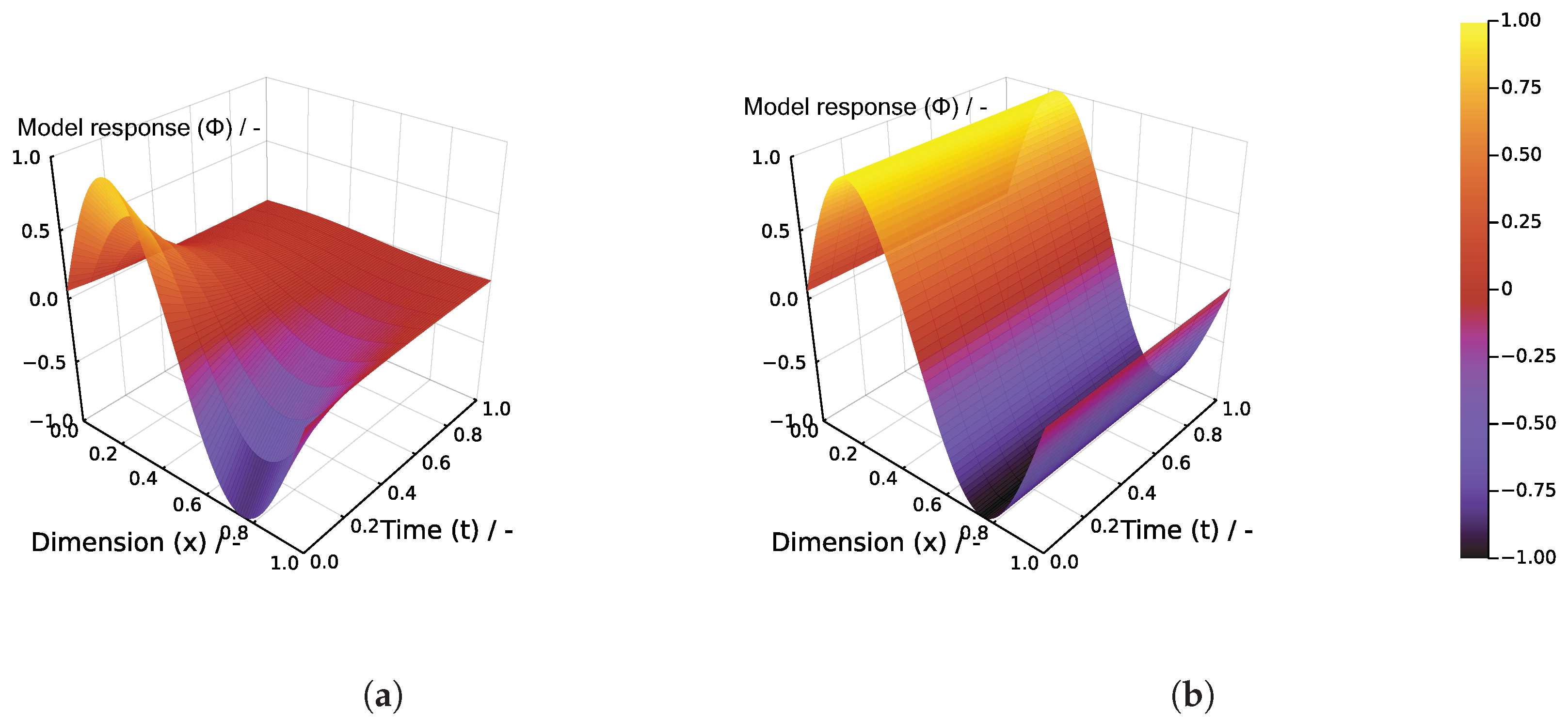
3.1. Scenario 1: Distributed Control Problem

In this case, it is assumed that all states in Equation (21), i.e., $y_i={\mathrm{\Phi }}_i,\forall 1\le i\le N$, are measurable and controllable, and that the output derivatives, i.e., ${\dot{y}}_i,\forall 1\le i\le N$, exist. Then the corresponding equation system (Equation (22)) can be converted to express the input variables, $u_i,\forall 1\le i\le N$, analytically [31].

$$\begin{array}{ccc}\hfill \left(\begin{array}{c}{\dot{y}}_1\left(t\right)\\ {\dot{y}}_2\left(t\right)\\ \cdots \\ {\dot{y}}_{N-1}\left(t\right)\\ {\dot{y}}_N\left(t\right)\end{array}\right)& =& \left(\begin{array}{ccccccccc}-\frac{2\kappa }{\mathsf{\Delta }{\mathbf{x}}^2}& \frac{\kappa }{\mathsf{\Delta }{\mathbf{x}}^2}& 0& 0& \cdots & 0& 0& 0& 0\\ \frac{\kappa }{\mathsf{\Delta }{\mathbf{x}}^2}& -\frac{2\kappa }{\mathsf{\Delta }{\mathbf{x}}^2}& \frac{\kappa }{\mathsf{\Delta }{\mathbf{x}}^2}& 0& \cdots & 0& 0& 0& 0\\ 0& \frac{\kappa }{\mathsf{\Delta }{\mathbf{x}}^2}& -\frac{2\kappa }{\mathsf{\Delta }{\mathbf{x}}^2}& \frac{\kappa }{\mathsf{\Delta }{\mathbf{x}}^2}& \cdots & 0& 0& 0& 0\\ \cdots & \cdots & \cdots & \cdots & \cdots & \cdots & \cdots & \cdots & \cdots \\ 0& 0& 0& 0& \cdots & 0& \frac{\kappa }{\mathsf{\Delta }{\mathbf{x}}^2}& -\frac{2\kappa }{\mathsf{\Delta }{\mathbf{x}}^2}& \frac{\kappa }{\mathsf{\Delta }{\mathbf{x}}^2}\\ 0& 0& 0& 0& \cdots & 0& 0& \frac{\kappa }{\mathsf{\Delta }{\mathbf{x}}^2}& -\frac{2\kappa }{\mathsf{\Delta }{\mathbf{x}}^2}\end{array}\right)\left(\begin{array}{c}{y}_1\left(t\right)\\ y_2\left(t\right)\\ \cdots \\ y_{N-1}\left(t\right)\\ y_N\left(t\right)\end{array}\right)+\hfill \\ & & \left(\begin{array}{cccccc}1& 0& 0& \cdots & 0& 0\\ 0& 1& 0& \cdots & 0& 0\\ 0& 0& 1& \cdots & 0& 0\\ \cdots & \cdots & \cdots & \cdots & \cdots & \cdots \\ 0& 0& 0& \cdots & 1& 0\\ 0& 0& 0& \cdots & 0& 1\end{array}\right)\left(\begin{array}{c}{u}_1\left(t\right)\\ u_2\left(t\right)\\ u_3\left(t\right)\\ \cdots \\ u_{N-1}\left(t\right)\\ u_N\left(t\right)\end{array}\right).\hfill \end{array}$$

(22)

Furthermore, when dealing with measurement data, instead of the full model system (Equation (22)), the neural ODE framework (Equation (13)) is used as a surrogate model to approximate the output functions and their derivatives. Specifically, the following multi-layer perceptron (MLP) setting is applied: two hidden layers with 400 nodes each, input and output layer with 198 nodes each, and $tanh$ as activation function. In order to train the neural ODE system, we use simulated data with $t_{i+1}-t_i=0.1,\mathsf{\Delta }\mathbf{x}=0.01,t\in [0,2],\mathbf{x}\in [0,1],\mathrm{\Phi }(t_0,\mathbf{x})=sin\left(2\pi \mathbf{x}\right),\mathrm{\Phi }(t,\mathbf{x}=0)=0,\mathrm{\Phi }(t,\mathbf{x}=1)=0,$ and $\kappa =0.1$ in dimensionless form.

3.2. Scenario 2: Boundary Control Problem

Unlike the distributed control problem, in this scenario, the distributed system is controlled by steering the right boundary (final) value towards the other end and using it as the control model input. It is important to consider this because, for physical assets, the states could be estimated using observers or filters with many techniques in control theory. However, practically speaking, not all of the system states could be measured using sensors with great precision. In such situations, the idea discussed above might not be very reliable when it comes to a parameter identification problem or a control problem. Often, only the boundary values could be accessed, depending on the measurement tools and their installations. Firstly, MOL technique (see Equation (2)) is implemented to transform the PDE system into a set of equivalent ODEs. These are then checked to satisfy the conditions for differential flatness [31]. The boundary condition in the ODE subsystem (usually comprising the last rows of the state space description) is the aggregate control input. The boundary control input is computed from the last element of the system state vector of the ODE subsystem to the first one.

However, in this study, it is assumed that the values of the right boundary are measured as accurately as possible. With this available data set, the flatness concept is also used to estimate the internal states of the system, the necessary control input, and initial values using backward calculation; see Equation (23).

Figure 4 shows the pictogram of a simple diffusion system. The input u, fed to the system from the left boundary (LB), diffuses throughout the dimensional space $\mathbf{x}$ (ranging from 0 to N). The only available measurement is y and the estimates (of the internal states) are denoted as ${\widehat{\mathrm{\Phi }}}_0$ to ${\widehat{\mathrm{\Phi }}}_{N-1}$. The left and right boundaries are represented as ${\varphi }_0$ and ${\varphi }_{N+1}$, respectively.

For this boundary problem scenario, the objective is to obtain a linear increase in the output values of the system at the right boundary ${\varphi }_{N+1}$, leading to a linear increase in the input boundary. A simple constant output trajectory is not desired here because it might lead to an ill-posed identification problem. Hence, this choice of a linear output profile is desired, as it will simplify the model inversion process by using only the first derivative, thereby avoiding the higher derivatives. This also has the advantage of not having a strong noise amplification, thus minimizing the control challenge without any need for filters and, consequently, their additional parameter tunings. The desired control input, initial values, and internal states could be determined using the following equation for backward calculation:

$$\begin{array}{ccc}\hfill y& =& {\varphi }_{N+1},\hfill \\ \hfill {\widehat{\mathrm{\Phi }}}_{N-1}& =& \frac{1}{D}(m+2D{y}_N-D{\varphi }_{N+1})=\frac{m}{D}+{\varphi }_{N+1},\hfill \\ \hfill {\widehat{\mathrm{\Phi }}}_{N-2}& =& \frac{1}{D}(m+2D{\widehat{\mathrm{\Phi }}}_{N-1}-D{y}_N)=\frac{3m}{D}+{\varphi }_{N+1},\hfill \\ \hfill {\widehat{\mathrm{\Phi }}}_{N-3}& =& \frac{1}{D}(m+2D{\widehat{\mathrm{\Phi }}}_{N-2}-D{\widehat{\mathrm{\Phi }}}_{N-1})=\frac{5m}{D}+{\varphi }_{N+1},\hfill \\ \hfill ⋮\\ \hfill {\widehat{\mathrm{\Phi }}}_1& =& \frac{1}{D}(m+2D{\widehat{\mathrm{\Phi }}}_2-D{\widehat{\mathrm{\Phi }}}_3)=\frac{(2n-3)m}{D}+{\varphi }_{N+1},\hfill \\ \hfill {\widehat{\mathrm{\Phi }}}_0& =& \frac{1}{D}(m+2D{\widehat{\mathrm{\Phi }}}_1-D{\widehat{\mathrm{\Phi }}}_2)=\frac{(2n-1)m}{D}+{\varphi }_{N+1}=u\left(t\right),\hfill \end{array}$$

(23)

where $D=\frac{\kappa }{\mathsf{\Delta }{\mathbf{x}}^2}$, m is the slope of the desired linearly increasing output, and $n=N-i$ with $i\in [1,N]$; see Equation (2). In this case, the boundary is assumed to be the same as that of the first and last states.

Thus, the distributed and boundary controls of the considered diffusion system are achieved using the flatness property of the measures. The generated control input is then used for analyzing its sensitivity (uses ILS formulation w.r.t. the diffusion paramere $\kappa$), which in turn, could be employed for parameter identification, consequently.

4. Results and Discussion

With the available measures, the internal states and the desired control inputs are estimated for both scenarios using the flatness concept, as discussed in Section 3. The results (with the assumed specifications) are presented, and the interpretations are analyzed henceforth. Initially, backward calculations using the flatness concept are presented to show the determined control inputs for both scenarios. This is followed by sensitivity analyses of the diffusion parameter w.r.t. the output (OLS) and the calculated input (ILS), and both are compared for efficacy.

4.1. Model Inversion via Differential Flatness

The diffusion dynamics (Equation (19)) is simulated forward to visualize the diffusion output phenomenon for a chosen diffusion coefficient. The two scenarios, i.e., distributed control and boundary control, are implemented based on Equations (22) and (23), and thus the control inputs are determined. Relevant graphs are presented for further discussion in terms of parameter sensitivity and parameter identifiability, respectively.

4.1.1. Scenario 1: Distributed Control Problem

For a simple diffusion dynamics (Equation (19)), forward simulation is done with the following setting: distributed control action $u\left(t\right)=0$, diffusion coefficient $\kappa =0.1$, initial condition $u(\mathbf{x},0)=sin2\pi \mathbf{x}$, Dirichlet boundary conditions $u(0,t)=0$ and $u(N,t)=0$ with $\mathbf{x}\in [0,N]$. The result of the simulation is shown in Figure 5a. The effect of diffusion can be seen very clearly, i.e., the initial differences along the spatial axis $\mathbf{x}$ at the start time, $y(t_0,\mathbf{x})$, decrease over the simulation time. Consequently, a variation of the diffusion parameter $\kappa$ would lead to a different diffusion profile based on the parameter sensitivity effect. It should be noted that in principle, due to parameter sensitivity, it is possible to identify the model parameter when applying OLS with experimental data and Equation (4). Alternatively, the differential flatness approach can be used to impose the desired process behavior. For this purpose, the parameter-dependent recalculated input variables allow parameter estimation following the ILS concept mentioned; see Equation (6).

In Figure 5b, for example, the output profile does not show changes over time. Please note that the required control input was predicted by making use of the flatness concept, the neural ODE system, and the given training scenario. Thus, in this case, the implementation of distributed control is shown by successfully controlling all measured states using differential flatness.

4.1.2. Scenario 2: Boundary Control Problem

For the diffusion dynamics in Equation (19) the output could be measured only at the right boundary ${\varphi }_{N+1}=y$. For this study, the output is desired to be linearly increasing at ${\varphi }_{N+1}$ from 20 to 30 units with a slope $m=10$ over one time unit. No other information about the system or its dynamics is available. However, the necessary control input is determined using Equation (23), along with the initial values, which are required for the forward simulation of the dynamics. Moreover, the estimated internal states of the system, as calculated back using Equation (23), are initially shown in the spatial domain at selected time instants t, in Figure 6a. The same estimated states are again plotted (dotted lines) in the time domain at selected points in the dimensional space x, for better interpretation, in Figure 6b. The forward simulation is then performed (Equation (19)), to check if the data determined using Equation (23) are precise. The following setting is adapted: diffusion coefficient $\kappa =0.1$, control input $u\left(t\right)$ and initial conditions $u(\mathbf{x},0)$ are applied from the estimations, Robin boundary conditions $u(0,t)=0$, $u^{\prime }(N,t)=1$ with $\mathbf{x}\in [0,N]$. The output profiles are plotted over time in the same selected points over x for better comprehension. The comparison can be found in Figure 6b.

The output (desired) at the measurable boundary increases linearly from 20 to 30 units (the green dotted line at $\widehat{\mathrm{\Phi }}$ at $\mathbf{x}=1.0$) (see Figure 6b). Then, the necessary feed at the input end should be 70 to 80 units (the red dotted line $\widehat{\mathrm{\Phi }}$ at $\mathbf{x}=0.0$) (see Figure 6b). The initial condition at $t=0.0$ is supposed to be diffusing from 70 to 20 units (the values of $\widehat{\mathrm{\Phi }}$ at $t=0.0$), which could be visualized as the black solid line $\widehat{\mathrm{\Phi }}$ at $t=0.0$ (see Figure 6a). Thus, by feeding the estimated control input u to the left boundary ${\varphi }_0$, the dynamics in Equation (19) are simulated with the estimated initial conditions. The resulting output profiles are presented as solid lines in Figure 6b, denoted by y at the same selective points across the dimensional space $\mathbf{x}$. It can be seen that the estimations $\widehat{\mathrm{\Phi }}$ at given x values match pretty closely with the output profiles y from the forward simulation. The model in Equation (19) is thus shown to be validated for the control input and initial conditions, which were determined from the boundary (flat) output by backward calculation using the flatness concept.

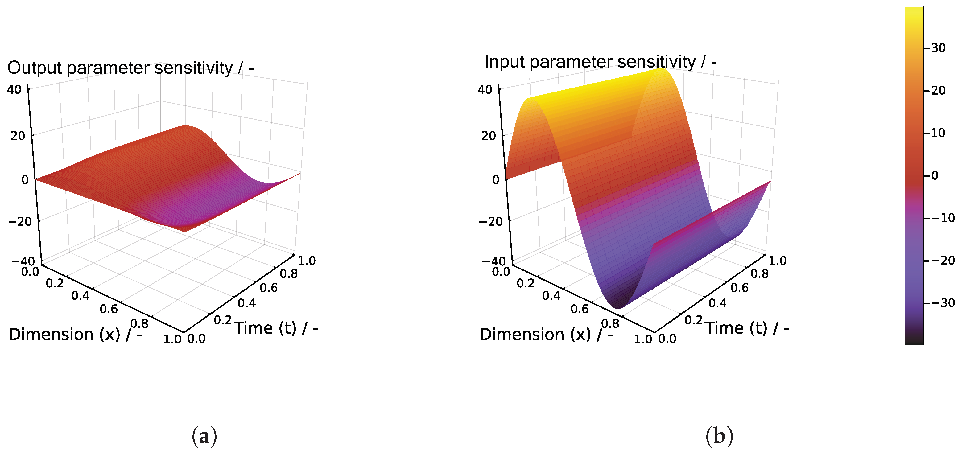
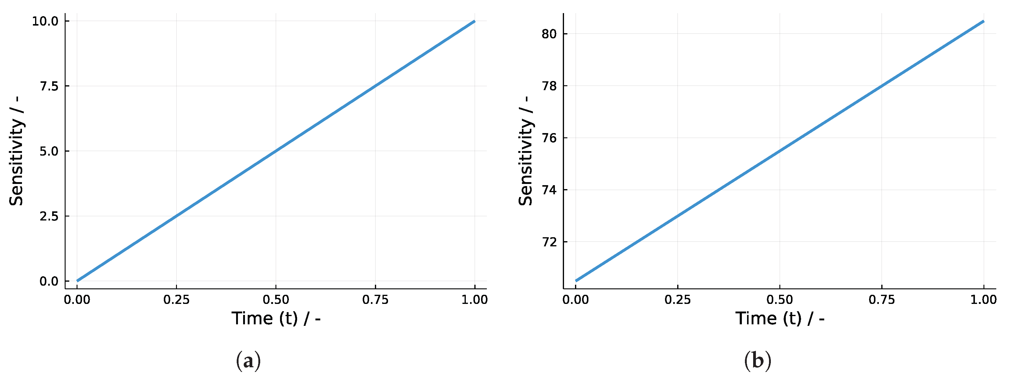
4.2. Sensitivity Analyses

The reconstructed input and output data generated from Figure 5b are used for the sensitivity analysis. The derived input function, like the output profile, depends on the diffusion parameter $\kappa$ and is thus sensitive to parameter changes. In the case of the output function and the generated control input, the sensitivities corresponding to a variation of the diffusion parameter $\kappa$ are studied using Equations (7) and (8). The study is done for both scenarios, and the corresponding interpretations are shown individually.

4.2.1. Scenarion 1: Distributed Control Problem

The sensitivities of the system output and the distributed control input (determined by model inversion) are analyzed for the diffusion parameter $\kappa$. In Figure 7, the corresponding sensitivity graphs are illustrated. Here, the output parameter sensitivity (Figure 7a) is zero for the starting point, and its absolute range is gradually rising at $\mathbf{x}=0.25$ and $\mathbf{x}=0.75$, respectively. In the case of the input parameter sensitivity (see Figure 7b), these sensitivities are at their peak from the very start, and their absolute values are 3–4 times higher than the sensitivities of the output parameter. This implies that the distributed control input is more informative than the system output for the diffusion parameter $\kappa$ estimation.

4.2.2. Scenario 2: Boundary Control Problem

The sensitivities of the desired boundary output and the boundary control input (backpropagation using differential flatness) for the diffusion parameter $\kappa$ are analyzed by comparing the sensitivity graphs in Figure 8. In Figure 8a, when parameter identification is to be defined using OLS (based on output), the absolute sensitivity values start from as low as 0 to a maximum of 10 over a time span of 1 unit. However, on the other hand, the boundary control input derived based on the flatness property is used to frame the cost function as ILS. Figure 8b shows that, while using ILS to define the parameter identification problem, the absolute values start immediately from a significantly higher value, around 70, and increase to 82 during the same simulation time span. Similar to the distributed control problem, this signifies that the boundary control input is more informative for the diffusion parameter $\kappa$ estimation than the boundary output.

In both scenarios, the model control inputs’ parameter sensitivities were much higher than those of the system outputs. As discussed in Section 2, higher parameter sensitivities, in turn, mean expected improvements in parameter accuracy. Therefore, parameter identification using the ILS scheme might be beneficial compared to the OLS scheme in terms of parameter reliability. This effect can also be physically explained. Most technical systems show smoothing behavior and thus act as a kind of low-pass filter for system excitations and system changes, i.e., disturbances are mitigated, which includes parameter variations. The model inversion, in turn, uses the opposite effect and thus clearly shows a more significant response with respect to parameter changes. However, this is also true for measurement noise when these methods are used for parameter estimation. The time derivatives of the model output functions (flat outputs) that are necessary for the model inversion lead to an amplification of the measurement noise. To what extent the amplification of the measurement noise compensates for the more favorable parameter sensitivity properties of the ILS or TLS methods is out of the scope of this work. The obtained results also allow a further explanation of the favorable parameter estimation properties of the PINN method, i.e., just by evaluating the governing equation mismatch ${\mathcal{L}}^{\mathrm{ode}}$ (Equation (16)) higher parameter sensitivities are likely because of the very same reasons as for the proposed model inversion concept.

5. Conclusions

Identifying model parameters is a fundamental problem in control and systems theory. This work demonstrates that the input least squares (ILS) and ordinary least squares (OLS) strategies for parameter identification result in different parameter sensitivities. Here, an improved parameter sensitivity range is observed for ILS. The original contribution is the meaningful combination of the differential flatness concept with neural ordinary differential equations and, in terms of model inversion, its general implication for data-driven engineering problems. We successfully applied our method for two relevant scenarios of a one-dimensional diffusion-type problem using synthetic data. Due to a maximized parameter sensitivity range, the loss function based on ILS might lead to a more precise estimation of the model parameter compared to the OLS-based parameter identification framework. The ILS implementation and the underlying neural ODE system are specifically designed for the considered problem and thus not yet efficiently transferable for new tasks—an aspect addressed in ongoing research. Future work will also focus on advanced model inversion schemes, not limited to differentially flat systems, and their robustness under relevant uncertainties, i.e., process and measurement noise.

References

1. Gernaey, K.V.; Cervera-Padrell, A.E.; Woodley, J.M. A perspective on PSE in pharmaceutical process development and innovation. Comput. Chem. Eng. 2012, 42, 15–29. [Google Scholar] [CrossRef]
2. Chen, Y.; Yang, O.; Sampat, C.; Bhalode, P.; Ramachandran, R.; Ierapetritou, M. Digital Twins in Pharmaceutical and Biopharmaceutical Manufacturing: A Literature Review. Processes 2020, 8, 1088. [Google Scholar] [CrossRef]
3. Udugama, I.A.; Bayer, C.; Baroutian, S.; Gernaey, K.V.; Yu, W.; Young, B.R. Digitalisation in chemical engineering: Industrial needs, academic best practice, and curriculum limitations. Educ. Chem. Eng. 2022, 39, 94–107. [Google Scholar] [CrossRef]
4. Batchu, S.P.; Hernandez, B.; Malhotra, A.; Fang, H.; Ierapetritou, M.; Vlachos, D.G. Accelerating manufacturing for biomass conversion via integrated process and bench digitalization: A perspective. React. Chem. Eng. 2022, 7, 813–832. [Google Scholar] [CrossRef]
5. Bonvin, D.; Georgakis, C.; Pantelides, C.; Barolo, M.; Rodrigues, D.; Schneider, R.; Dochain, D.; Grover, M. Linking Models and Experiments. Ind. Eng. Chem. Res. 2016, 55. [Google Scholar] [CrossRef]
6. Yang, S.; Navarathna, P.; Ghosh, S.; Bequette, B.W. Hybrid Modeling in the Era of Smart Manufacturing. Comput. Chem. Eng. 2020, 140, 106874. [Google Scholar] [CrossRef]
7. Nielsen, R.F.; Nazemzadeh, N.; Sillesen, L.W.; Andersson, M.P.; Gernaey, K.V.; Mansouri, S.S. Hybrid machine learning assisted modelling framework for particle processes. Comput. Chem. Eng. 2020, 140, 106916. [Google Scholar] [CrossRef]
8. Chao, M.A.; Kulkarni, C.; Goebel, K.; Fink, O. Fusing physics-based and deep learning models for prognostics. Reliab. Eng. Syst. Saf. 2022, 217, 107961. [Google Scholar] [CrossRef]
9. Azadi, P.; Winz, J.; Leo, E.; Klock, R.; Engell, S. A hybrid dynamic model for the prediction of molten iron and slag quality indices of a large-scale blast furnace. Comput. Chem. Eng. 2022, 156, 107573. [Google Scholar] [CrossRef]
10. Sharma, N.; Liu, Y.A. A hybrid science-guided machine learning approach for modeling chemical processes: A review. AIChE J. 2022, 68, e17609. [Google Scholar] [CrossRef]
11. Razavi, S.; Jakeman, A.; Saltelli, A.; Prieur, C.; Iooss, B.; Borgonovo, E.; Plischke, E.; Lo Piano, S.; Iwanaga, T.; Becker, W.; et al. The Future of Sensitivity Analysis: An Essential Discipline for Systems Modeling and Policy Support. Environ. Model. Softw. 2020, 137, 104954. [Google Scholar] [CrossRef]
12. Rudin, C. Stop Explaining Black Box Machine Learning Models for High Stakes Decisions and Use Interpretable Models Instead. Nat. Mach. Intell. 2019, 1, 206–215. [Google Scholar] [CrossRef] [PubMed]
13. Samek, W.; Müller, K.R. Towards Explainable Artificial Intelligence; Springer: Cham, Switzerland, 2019; pp. 5–22. [Google Scholar] [CrossRef]
14. Bradley, W.; Kim, J.; Kilwein, Z.; Blakely, L.; Eydenberg, M.; Jalvin, J.; Laird, C.; Boukouvala, F. Perspectives on the Integration between First-Principles and Data-Driven Modeling. Comput. Chem. Eng. 2022, in press. [Google Scholar] [CrossRef]
15. Bhonsale, S.; Stokbroekx, B.; Van Impe, J. Assessment of the parameter identifiability of population balance models for air jet mills. Comput. Chem. Eng. 2020, 143, 107056. [Google Scholar] [CrossRef]
16. Villaverde, A.; Pathirana, D.; Froehlich, F.; Hasenauer, J.; Banga, J. A protocol for dynamic model calibration. Brief. Bioinform. 2021, 23, bbab387. [Google Scholar] [CrossRef]
17. Wieland, F.G.; Hauber, A.; Rosenblatt, M.; Tönsing, C.; Timmer, J. On structural and practical identifiability. Curr. Opin. Syst. Biol. 2021, 25, 60–69. [Google Scholar] [CrossRef]
18. Walter, E.; Norton, J.; Pronzato, L. Identification of Parametric Models: From Experimental Data; Communications and Control Engineering; Springer: Berlin/Heidelberg, Germany, 1997. [Google Scholar]
19. Abt, V.; Barz, T.; Cruz, N.; Herwig, C.; Kroll, P.; Möller, J.; Pörtner, R.; Schenkendorf, R. Model-based tools for optimal experiments in bioprocess engineering. Curr. Opin. Chem. Eng. 2018, 22, 244–252. [Google Scholar] [CrossRef]
20. Krausch, N.; Barz, T.; Kemmer, A.; Kamel, S.; Neubauer, P.; Cruz Bournazou, M. Monte Carlo Simulations for the Analysis of Non-linear Parameter Confidence Intervals in Optimal Experimental Design. Front. Bioeng. Biotechnol. 2019, 7, 122. [Google Scholar] [CrossRef]
21. Nimmegeers, P.; Bhonsale, S.; Telen, D.; Van Impe, J. Optimal experiment design under parametric uncertainty: A comparison of a sensitivities based approach versus a polynomial chaos based stochastic approach. Chem. Eng. Sci. 2020, 221, 115651. [Google Scholar] [CrossRef]
22. Schenkendorf, R.; Xie, X.; Rehbein, M.; Scholl, S.; Krewer, U. The Impact of Global Sensitivities and Design Measures in Model-Based Optimal Experimental Design. Processes 2018, 6, 27. [Google Scholar] [CrossRef]
23. Francis-Xavier, F.; Kubannek, F.; Schenkendorf, R. Hybrid Process Models in Electrochemical Syntheses under Deep Uncertainty. Processes 2021, 9, 704. [Google Scholar] [CrossRef]
24. Barz, T.; López, C.D.; Cruz Bournazou, M.; Körkel, S.; Walter, S. Real-time adaptive input design for the determination of competitive adsorption isotherms in liquid chromatography. Comput. Chem. Eng. 2016, 94, 104–116. [Google Scholar] [CrossRef]
25. Bhatt, N.; Kerimoglu, N.; Amrhein, M.; Marquardt, W.; Bonvin, D. Incremental Identification of Reaction Systems—A Comparison between Rate-based and Extent-based Approaches. Chem. Eng. Sci. 2012, 83, 24–38. [Google Scholar] [CrossRef]
26. Poyton, A.; Varziri, M.; McAuley, K.; Mclellan, P.; Ramsay, J. Parameter Estimation in Continuous-Time Dynamic Models Using Principal Differential Analysis. Comput. Chem. Eng. 2006, 30, 698–708. [Google Scholar] [CrossRef]
27. Varziri, M.; Poyton, A.; McAuley, K.; McLellan, P.; Ramsay, J. Selecting optimal weighting factors in iPDA for parameter estimation in continuous-time dynamic models. Comput. Chem. Eng. 2008, 32, 3011–3022. [Google Scholar] [CrossRef]
28. Schenkendorf, R.; Mangold, M. Parameter Identification for Ordinary and Delay Differential Equations by Using Flat Inputs. Theor. Found. Chem. Eng. 2014, 48, 594–607. [Google Scholar] [CrossRef]
29. Liu, J.; Mendoza, S.; Li, G.; Fathy, H. Efficient Total Least Squares State and Parameter Estimation for Differentially Flat Systems. In Proceedings of the 2016 American Control Conference (ACC), Boston, MA, USA, 6–8 July 2016; pp. 5419–5424. [Google Scholar] [CrossRef]
30. Fliess, M.; Lévine, J.; Martin, P.; Rouchon, P. Flatness and defect of non-linear systems: Introductory theory and examples. Int. J. Control 1995, 61, 13–27. [Google Scholar] [CrossRef]
31. Rigatos, G.G. Nonlinear Control and Filtering Using Differential Flatness Approaches; Springer: Cham, Switzerland, 2015. [Google Scholar]
32. Liu, J.; Li, G.; Fathy, H. A Computationally Efficient Approach for Optimizing Lithium-Ion Battery Charging. J. Dyn. Syst. Meas. Control. 2015, 138, 021009. [Google Scholar] [CrossRef]
33. Blechschmidt, J.; Ernst, O.G. Three ways to solve partial differential equations with neural networks—A review. GAMM-Mitteilungen 2021, 44, e202100006. [Google Scholar] [CrossRef]
34. Markidis, S. The Old and the New: Can Physics-Informed Deep-Learning Replace Traditional Linear Solvers? arXiv 2021, arXiv:2103.09655. [Google Scholar] [CrossRef]
35. Raissi, M.; Perdikaris, P.; Karniadakis, G. Physics-Informed Neural Networks: A Deep Learning Framework for Solving Forward and Inverse Problems Involving Nonlinear Partial Differential Equations. J. Comput. Phys. 2018, 378, 686–707. [Google Scholar] [CrossRef]
36. Yazdani, A.; Lu, L.; Raissi, M.; Karniadakis, G.E. Systems biology informed deep learning for inferring parameters and hidden dynamics. PLoS Comput. Biol. 2020, 16, e1007575. [Google Scholar] [CrossRef]
37. Yang, L.; Meng, X.; Karniadakis, G.E. B-PINNs: Bayesian physics-informed neural networks for forward and inverse PDE problems with noisy data. J. Comput. Phys. 2021, 425, 109913. [Google Scholar] [CrossRef]
38. Zubov, K.; McCarthy, Z.; Ma, Y.; Calisto, F.; Pagliarino, V.; Azeglio, S.; Bottero, L.; Luján, E.; Sulzer, V.; Bharambe, A.; et al. NeuralPDE: Automating Physics-Informed Neural Networks (PINNs) with Error Approximations. arXiv 2021, arXiv:2107.09443. [Google Scholar] [CrossRef]
39. Chen, R.T.Q.; Rubanova, Y.; Bettencourt, J.; Duvenaud, D. Neural Ordinary Differential Equations. arXiv 2018, arXiv:1806.07366. [Google Scholar] [CrossRef]
40. Kaiser, E.; Kutz, J.N.; Brunton, S.L. Data-driven approximations of dynamical systems operators for control. arXiv 2019, arXiv:1902.10239. [Google Scholar] [CrossRef]
41. Champion, K.; Lusch, B.; Kutz, J.N.; Brunton, S.L. Data-driven discovery of coordinates and governing equations. Proc. Natl. Acad. Sci. USA 2019, 116, 22445–22451. [Google Scholar] [CrossRef]
42. Lee, K.; Trask, N.; Stinis, P. Structure-preserving Sparse Identification of Nonlinear Dynamics for Data-driven Modeling. arXiv 2021, arXiv:2109.05364. [Google Scholar] [CrossRef]
43. Owoyele, O.; Pal, P. ChemNODE: A neural ordinary differential equations framework for efficient chemical kinetic solvers. Energy AI 2022, 7, 100118. [Google Scholar] [CrossRef]
44. Fasel, U.; Kutz, J.N.; Brunton, B.W.; Brunton, S.L. Ensemble-SINDy: Robust sparse model discovery in the low-data, high-noise limit, with active learning and control. Proc. R. Soc. A Math. Phys. Eng. Sci. 2022, 478, 20210904. [Google Scholar] [CrossRef]
45. Selvarajan, S.; Tappe, A.; Heiduk, C.; Scholl, S.; Schenkendorf, R. Parameter Identification Concept for Process Models Combining Systems Theory and Deep Learning. Eng. Proc. 2022, 19, 27. [Google Scholar] [CrossRef]
46. Bird, R.B.; Stewart, W.E.; Lightfoot, E.N. Transport Phenomena; Number Bd. 1 in Transport Phenomena; Wiley: Hoboken, NJ, USA, 2006. [Google Scholar]
47. Schiesser, W. The Numerical Method of Lines: Integration of Partial Differential Equations; Academic Press: Cambridge, MA, USA, 1991. [Google Scholar]
48. Schiesser, W.; Griffiths, G. A Compendium of Partial Differential Equation Models; Cambridge University Press: Cambridge, UK, 2009. [Google Scholar] [CrossRef]
49. Baranowska, A.; Kamont, Z. Numerical Method of Lines for First Order Partial Differential-Functional Equations. Z. Anal. Ihre Anwend. 2002, 21, 949–962. [Google Scholar] [CrossRef]
50. Turányi, T.; Tomlin, A.S. Analysis of Kinetic Reaction Mechanisms; Springer: Berlin/Heidelberg, Germany, 2014; Volume 20. [Google Scholar]
51. Baader, F.J.; Althaus, P.; Bardow, A.; Dahmen, M. Demand Response for Flat Nonlinear MIMO Processes using Dynamic Ramping Constraints. arXiv 2022, arXiv:2205.14598. [Google Scholar]
52. Meurer, T. Flatness-based trajectory planning for diffusion-reaction systems in a parallelepipedon—A spectral approach. Automatica 2011, 47, 935–949. [Google Scholar] [CrossRef]
53. Kater, A.; Meurer, T. Motion planning and tracking control for coupled flexible beam structures. Control. Eng. Pract. 2019, 84, 389–398. [Google Scholar] [CrossRef]
54. Meurer, T. Control of Higher–Dimensional PDEs: Flatness and Backstepping Designs; Springer Science & Business Media: Berlin/Heidelberg, Germany, 2012. [Google Scholar]
55. Meurer, T.; Andrej, J. Flatness-based model predictive control of linear diffusion-convection-reaction processes. In Proceedings of the 2018 IEEE Conference on Decision and Control (CDC), Miami, FL, USA, 17–19 December 2018; pp. 527–532. [Google Scholar] [CrossRef]
56. Kolar, B.; Rams, H.; Schlacher, K. Time-optimal flatness based control of a gantry crane. Control Eng. Pract. 2017, 60, 18–27. [Google Scholar] [CrossRef]
57. Ge, S.; Lee, T.; Zhu, G. Energy-based robust controller design for multilink flexible robot. Mechatronics 1996, 6, 779–798. [Google Scholar] [CrossRef]
58. Rigatos, G. Advanced Models of Neural Networks: Nonlinear Dynamics and Stochasticity in Biological Neurons; Springer: Berlin/Heidelberg, Germany, 2014. [Google Scholar]
59. Rudolph, J.; Winkler, J.; Woittennek, F. Flatness Based Control of Distributed Parameter Systems: Examples and Computer Exercises from Various Technological Domains; Shaker Verlag: Düren, Germany, 2003. [Google Scholar]
60. Gustineli, M. A survey on recently proposed activation functions for Deep Learning. arXiv 2022, arXiv:2204.02921. [Google Scholar]
61. Rackauckas, C.; Innes, M.; Ma, Y.; Bettencourt, J.; White, L.; Dixit, V. DiffEqFlux.jl—A Julia Library for Neural Differential Equations. arXiv 2019, arXiv:1902.02376. [Google Scholar]
62. He, K.; Zhang, X.; Ren, S.; Sun, J. Deep Residual Learning for Image Recognition. In Proceedings of the IEEE Conference on Computer Vision and Pattern Recognition, Las Vegas, NV, USA, 27–30 June 2016; pp. 770–778. [Google Scholar] [CrossRef]
63. Lee, K.; Parish, E. Parameterized neural ordinary differential equations: Applications to computational physics problems. Proc. R. Soc. A Math. Phys. Eng. Sci. 2021, 477, 20210162. [Google Scholar] [CrossRef]
64. Rackauckas, C.; Ma, Y.; Martensen, J.; Warner, C.; Zubov, K.; Supekar, R.; Skinner, D.; Ramadhan, A. Universal Differential Equations for Scientific Machine Learning. arXiv 2020, arXiv:2001.04385. [Google Scholar]
65. Massaroli, S.; Poli, M.; Park, J.; Yamashita, A.; Asama, H. Dissecting Neural ODEs. arXiv 2020, arXiv:2002.08071. [Google Scholar] [CrossRef]
66. Wang, G.; Briskot, T.; Hahn, T.; Baumann, P.; Hubbuch, J. Estimation of adsorption isotherm and mass transfer parameters in protein chromatography using artificial neural networks. J. Chromatogr. A 2017, 1487, 211–217. [Google Scholar] [CrossRef]
67. Polis, M. The Distributed System Parameter Identification Problem: A Survey of Recent Results. IFAC Proc. Vol. 1983, 16, 45–58. [Google Scholar] [CrossRef]
68. Gehring, N.; Rudolph, J. An algebraic algorithm for parameter identification in a class of systems described by linear partial differential equations. PAMM 2016, 16, 39–42. [Google Scholar] [CrossRef]
69. Grimard, J.; Dewasme, L.; Vande Wouwer, A. A Review of Dynamic Models of Hot-Melt Extrusion. Processes 2016, 4, 19. [Google Scholar] [CrossRef] [Green Version]
Figure 1. Standard workflow of identifying model parameters in process modeling with n iterations.
Processes 10 01764 g001
Figure 2. Ordinary Least Squares (OLS) and Input Least Squares (ILS) workflow and their use of experimental data in terms of loss function definitions, process model parameter identification, and parameter sensitivities. For the ILS case, the two open problems, i.e., the definition of the empirical output function and the transformation step for the model input calculation, are highlighted, too.
Processes 10 01764 g002
Figure 3. Comparative scheme of the physics-informed neural network (PINN) approach with the proposed procedure combining neural ordinary differential equations (NODEs) and the inverse model (recalculated model input via differential flatness), including needed loss function definitions and the use of experimental data to identify unknown model parameters p and hyperparameters θ of the two different neural network architectures.
Processes 10 01764 g003
Figure 4. A standard diffusion-type boundary control problem (LB: Left boundary ϕ 0 ; RB: Right boundary ϕ N + 1 ; u: system input; y: system’s measurable output; Φ ^ : estimated states across x [ 0 , N ] : internal dimensional space of the system).
Processes 10 01764 g004
Figure 5. Model response for Scenario 1 assuming a distributed control problem with (a) when a zero input profile is applied (i.e., no control action that could counteract the diffusion effect) and with (b) when a purpose designed input is used to cancel out the diffusion effect; adapted from [45].
Processes 10 01764 g005
Figure 6. Model response for Scenario 2 assuming a boundary control problem with (a) for the recalculated diffusion profiles using the measured boundary value and (b) for the calculated diffusion profiles with the forward simulation output profiles.
Processes 10 01764 g006
Figure 7. Parameter sensitivity of the diffusion parameter κ for Scenario 1 assuming a distributed control problem with (a) using OLS to define the parameter identification problem and (b) where ILS is used to define the parameter identification problem instead.
Processes 10 01764 g007
Figure 8. Parameter sensitivity of the diffusion parameter κ for Scenario 2 assuming a boundary control problem with (a) using OLS to define the parameter identification problem and (b) where ILS is used to define the parameter identification problem instead.
Processes 10 01764 g008
Publisher’s Note: MDPI stays neutral with regard to jurisdictional claims in published maps and institutional affiliations.