Understanding Powder Behavior in an Additive Manufacturing Process Using DEM

Abstract

The handling of bulk solids in the form of powders is a fundamental process in a wide range of manufacturing industries, such as the automotive, aerospace, food, and healthcare sectors. All these sectors employ additive manufacturing (AM), as it enables the production of complex parts in a short amount of time. Thus, it is considered an established method for developing an agile manufacturing environment that can drastically reduce the lead time from conception to the production stage. At the same time, powder is a unique material sensitive to environmental and machine conditions; hence, establishing an optimal configuration is not straight-forward. This work presents a discrete element method (DEM) simulation of an experimental dosing system used in AM. We introduce a robust workflow that correlates suitable experimental data with simulation results, establishing models of real powders with different flowability. The results showed an excellent agreement between the experimental data and the simulation results and provided a better understanding of the material behavior. Furthermore, we employed a coarse-grained approach to extract continuum fields from the discrete data. The results showed that the cohesion level in the system was enough to create agglomerates that hindered the transport of the material and produced nonuniform distribution.

1. Introduction

Additive manufacturing (AM) has proved to be a novel production for a wide range of applications, such as aerospace, biology, medicine, and architecture [1,2,3,4]. This is because it is able to create three-dimensional parts directly from computer-aided design (3D CAD) without the need for expensive machinery, labor, and increased time. Its enormous potential for the rapid manufacturing of complex and customized parts has resulted in its exponential growth, including various manufacturing methods such as 3D printing from a liquid-based feed [5], powder spreading [6], laser sintering [7], and others.

Different types of powders, either in the form of pure powder or agglomerates, are the main materials used in such applications, and they are fed into various types of AM production equipment through delivery systems. The latter use prescribed volumes of powders and control their flow into the printer spreading systems, hence dictating the success or failure of the endproduct and influencing the machine set-up needed. Due to the small particle sizes that these powders have, they exhibit a host of processing problems, such as inconsistent flow, arching sensitivity to operational conditions, and others. Furthermore, it is critical to understand the effect of powder properties on the mechanics of the system and optimize the equipment.

The discrete element method (DEM) has been recognized as one of the most efficient numerical tools for solving various scientific and engineering problems. It is based on the work of Cundall and Strack [8], which represents particulate material as an assembly of discrete elements. The DEM uses the Lagrangian approach, in which particles of granular material are considered contacting bodies, and their dynamic parameters (position, velocity, orientation, etc.) are continuously tracked during the simulation. Therefore, the nature of the DEM is considered a very suitable tool when it comes to exploring the fundamentals of particle mechanics in additive manufacturing.

Fine powders are particularly challenging, with complex elasto-plastic-adhesive behavior that produces unwanted agglomeration phenomena hindering their flow. At the same time, performing experiments is challenging due to the opaque nature of the system. The methodology presented herein provides a deep understanding of the mechanics of such solids, making such simulations an indispensable tool for complex industrial applications. For this work, we used EDEM, which is a widely used commercial DEM code [9] previously verified against a set of benchmark tests by Chung and Ooi [10].

Delivery dosing systems aim to deliver a precise quantity of powder of high flowability for subsequent spreading, and the reliability of their performance strongly affects the finished product quality. The major design challenge is to ensure reliable and precise operation while processing powders of variable properties. Therefore, the focus of our work is on understanding the effects of powder properties and wheel rotational velocity on the accuracy of dosing and the quality of the powder-flow characteristics after dosing. To this end, EDEM is used to develop material models that replicate powders of two flowability extremes in the context of 3D printing and is used to simulate powder flow through the dosing wheel. Finally, a coarse-graining approach is implemented using EDEMPy to extract continuum fields from the discrete information and visualize the results in a continuum manner.

2. Numerical Methods

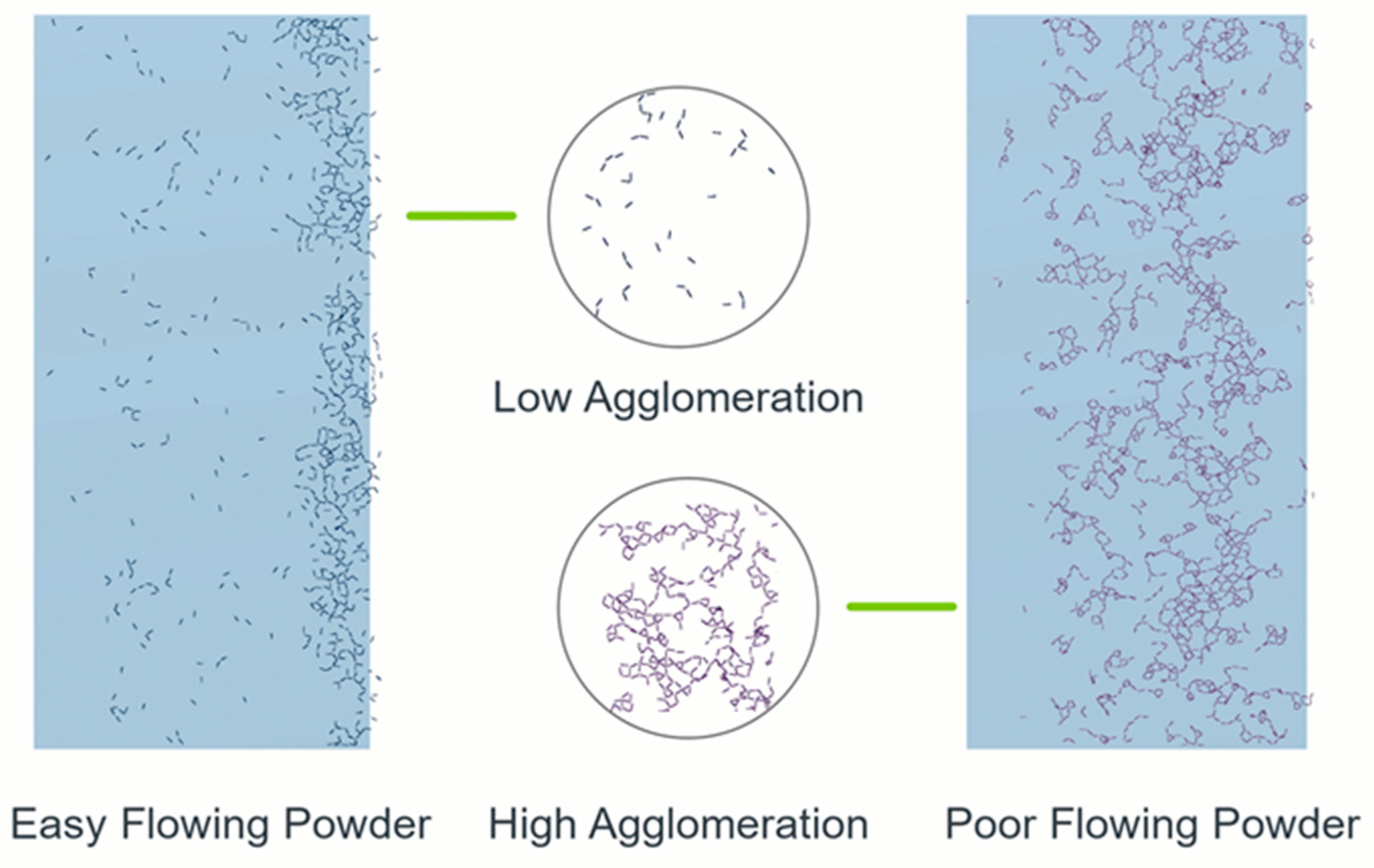
2.1. Material Modeling

Discrete element modeling for additive manufacturing powders of two flowability extremes was conducted in this work. The computational expense of modeling these materials at the physical particle scale was prohibitive, and a computationally efficient meso-scopic modeling approach was adopted whereby the material was modeled on an intermediate scale between the physical particle scale and the scale of the system of interest in order to achieve practical computational times. Previous work has shown that this approach can produce excellent quantitative predictions of the macromechanical behavior of fine-particulate solids under complex loading conditions [11,12].

Particle shape and size have significant effects on the bulk behavior of particulate solids, making them an important consideration in the DEM modeling of these materials [13]. In the context of mesoscopic modeling, however, the numerical particle represents an agglomeration of millions of physical particles, and replicating the physical particle morphology in the model becomes less meaningful. Indeed, previous works have shown that the use of a simple, two-sphere particle with an aspect ratio equal or greater than 1.25 can lead to excellent quantitative predictions of the macromechanical responses of powders under complex loading conditions. The same approach was adopted in this study, as shown in Figure 1.

2.2. Calibration of DEM Parameters

Mesoscopic modeling requires a contact model that can reproduce the macromechanical behavior of a particulate solid using the micromechanical parameters. Several models have been proposed [14,15], but the Edinburgh-elastic-plastic-adhesive model was adopted in this work, as it has been successfully applied before to model powders in both quasi-static and dynamic applications [11,16]. The micromechanical parameters of DEM contact models, in general, and mesoscopic contact models, in particular, are often difficult and sometimes impossible to measure directly. Therefore, an indirect determination of the appropriate values for these parameters is typically conducted in DEM modeling whereby the values are optimized to capture a carefully chosen macromechanical response in the model. Because the determination of the input parameter values is performed indirectly, the chosen experimental response for optimization needs to be sensitive to the same physical phenomena as the system of interest and should, therefore, induce a similar stress state and flow regime as the one expected in the system of interest. In this work, the widely used basic flowability energy (BFE) measurement of an FT4 powder rheometer was chosen for this purpose because it is conducted in a dynamic flow regime and under low stress magnitudes [17], which are the expected conditions in a dosing wheel.

A standard FT4 rheometer BFE test with a 50 mL vessel was modeled. The test measured the force and torque on the shaft of an impeller blade, which passed through a bed of powder in a helical downward motion, as illustrated in Figure 2. The movement of the blade was defined by the blade-tip speed, which was a function of the vertical velocity, rotational velocity, and helix angle of the blade. The modeling focused on an experimental test procedure at 100 mm/s blade-tip speed. The primary measurement of the instrument was the energy requirement for the downward helical motion of the blade, which was termed the basic flowability energy (BFE) and calculated according to Equation (1):

$$E_F={{\displaystyle \int }}_{Hmin}^{Hmax}\left(F_v+\frac{T}{rtan\left(a\right)}\right)dH$$

(1)

where $dH$ is the data write-out interval, $F_v$ is the resultant vertical force, $T$ is the torque, $r$ is the radius of the blade, and $a$ is the helix angle.

The conditioning cycle performed in the physical test prior to the BFE measurement was found to have a negligibly small effect on the computed results and was ignored in the interest of computational efficiency. The filling was modeled by the random rainfall method. The simulation stages are illustrated in Figure 3.

The model input parameter optimization was conducted in a staged approach. A parameter sensitivity analysis was conducted first by generating a set of twelve simulation runs in a Plackett–Burman design of experiment configuration and by fitting a linear response model to the data. The response model was then used to assess the relative importance of the input parameters with respect to the responses of interest, as well as to produce initial estimates of the appropriate input parameter values. A detailed description of the calibration methodology can be found in Pantaleev, et al. [11]. The computed BFE results are shown in Figure 4 and Figure 5. An excellent quantitative prediction of the evolution of the flow energy response was achieved in all the cases. The poured bulk densities of the two powders were also closely matched by the model, as shown in

Table 1. Physical bulk density and matched simulated results.

Material	Physical Bulk Density (g/mL)	Simulated Bulk Density (g/mL)
Powder 1	2.85	2.85
Powder 2	4.30	4.25

. The results were achieved with a relatively low number of simulations (18 in total), demonstrating the efficiency of the adopted calibration methodology.

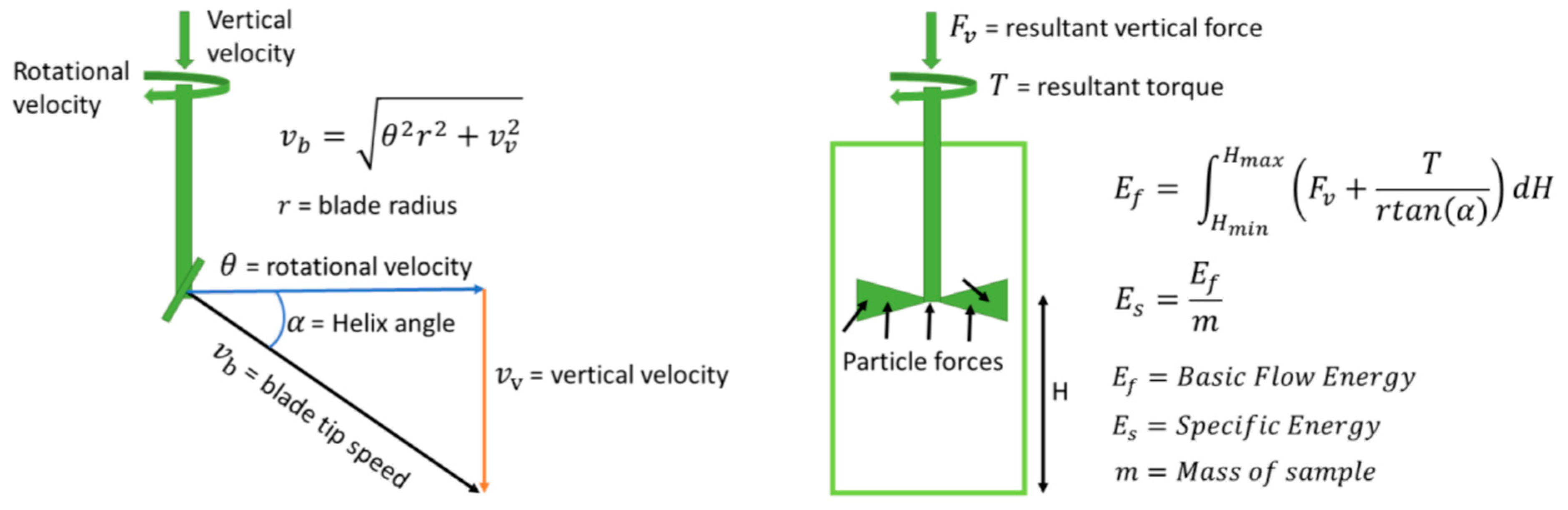
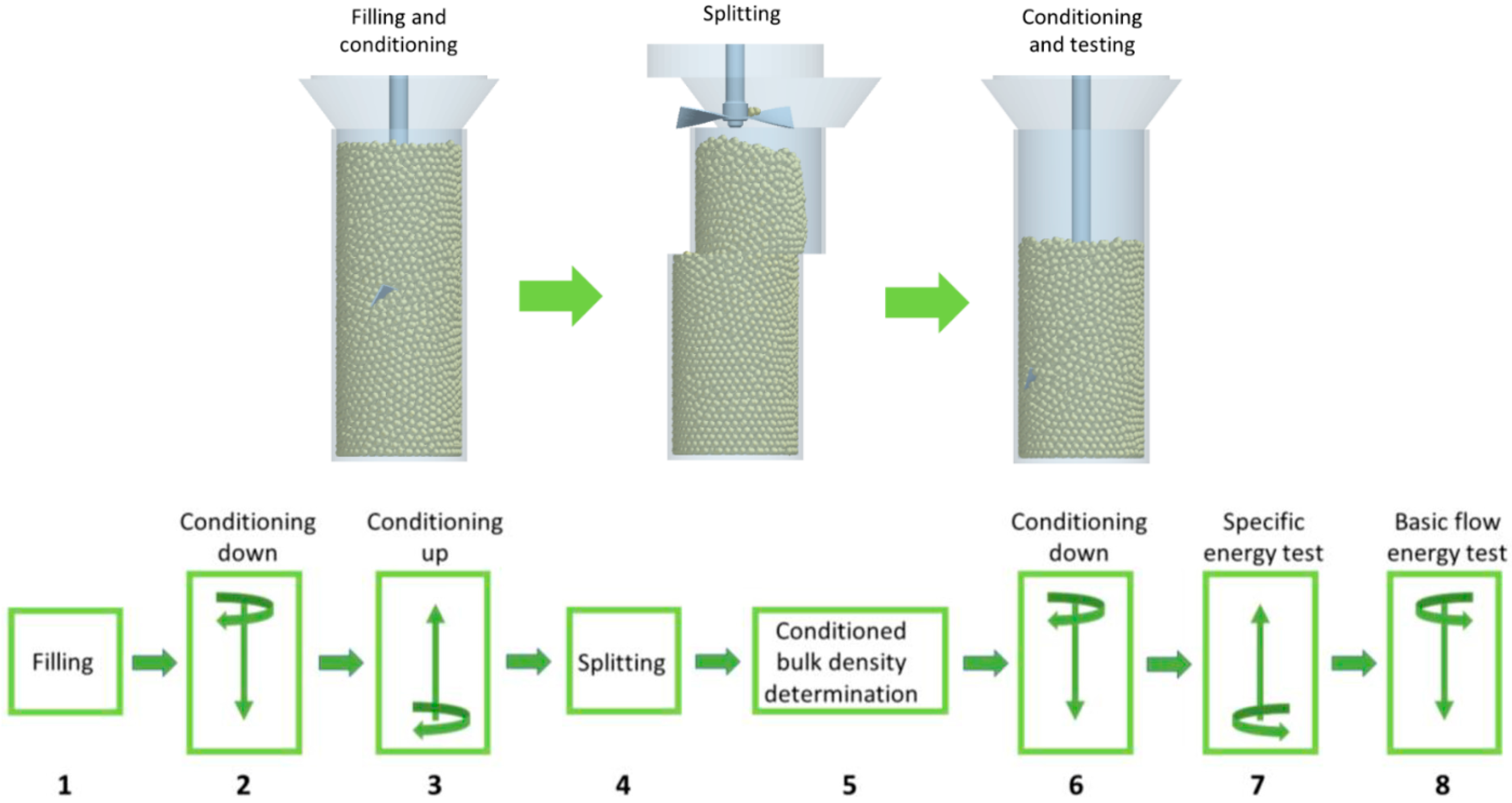
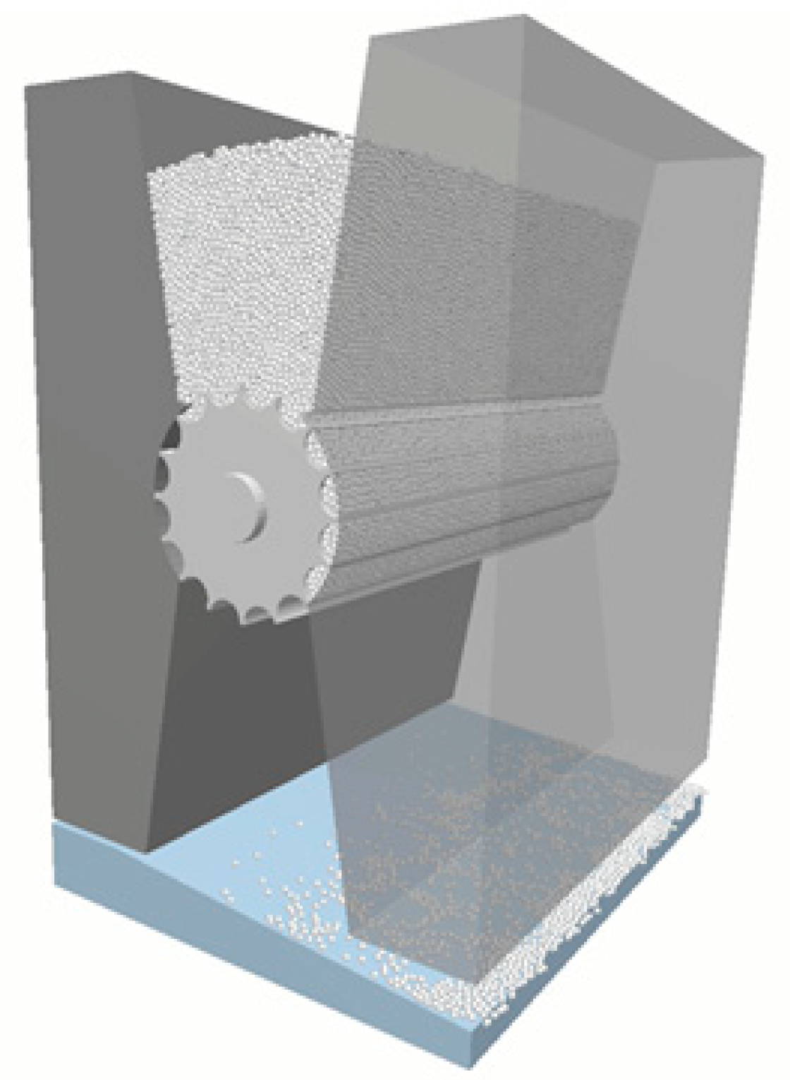
2.3. DEM Modeling of the Dosing Wheel Application

The filling and kinematics of the physical system were fully replicated in the DEM model, as shown in Figure 6. This involved the filling of the doser under gravity, followed by the discharge of the powder by the rotation of the dosing wheel onto a vibrating surface. Approximately 1.2 × 10⁵ bi-sphered particles were generated by the random rainfall method and were allowed to settle under gravity until a static powder bed was achieved. The dosing process was then simulated for 22 s of physical time. A graphic processing unit was used to accelerate the calculations.

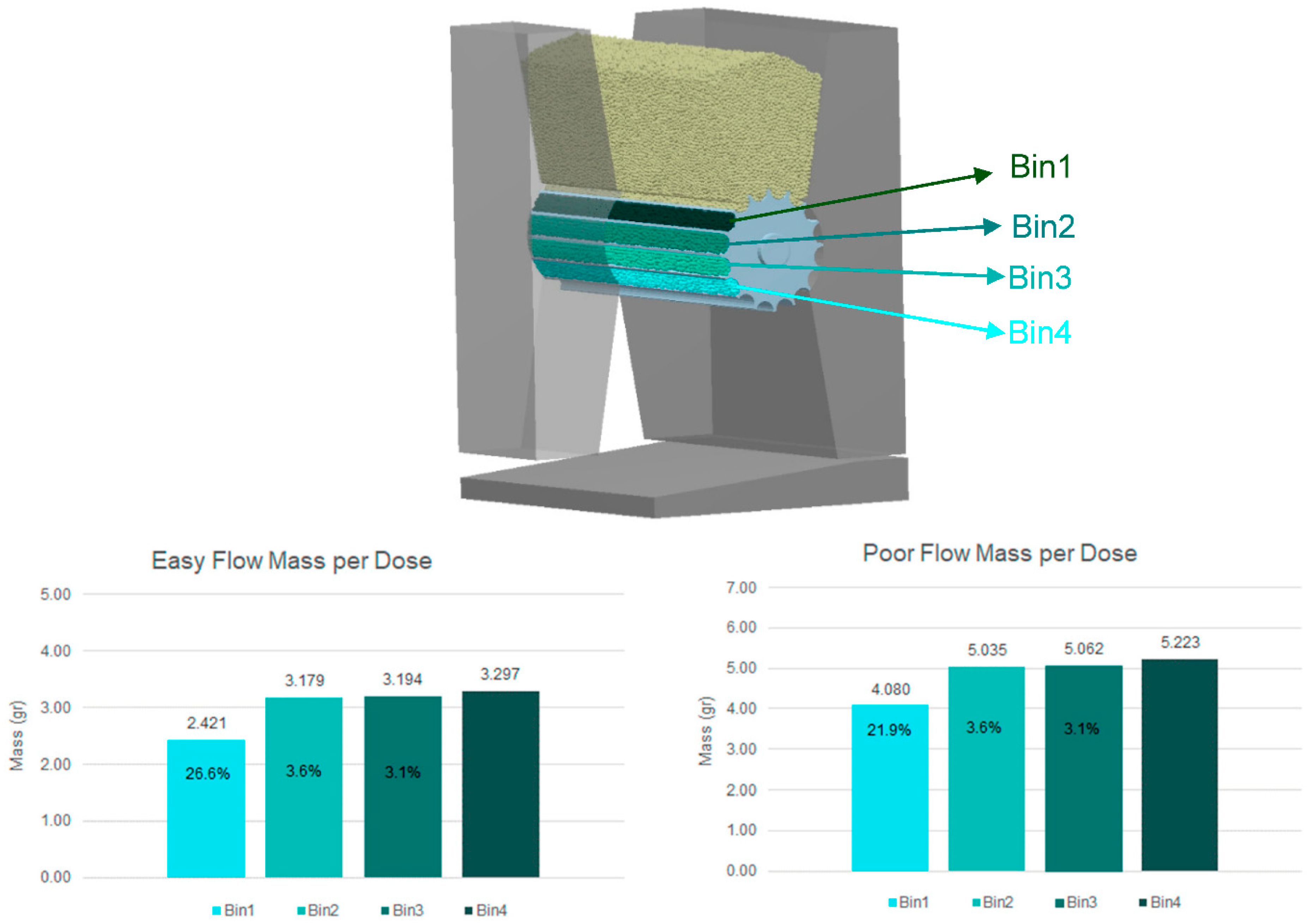
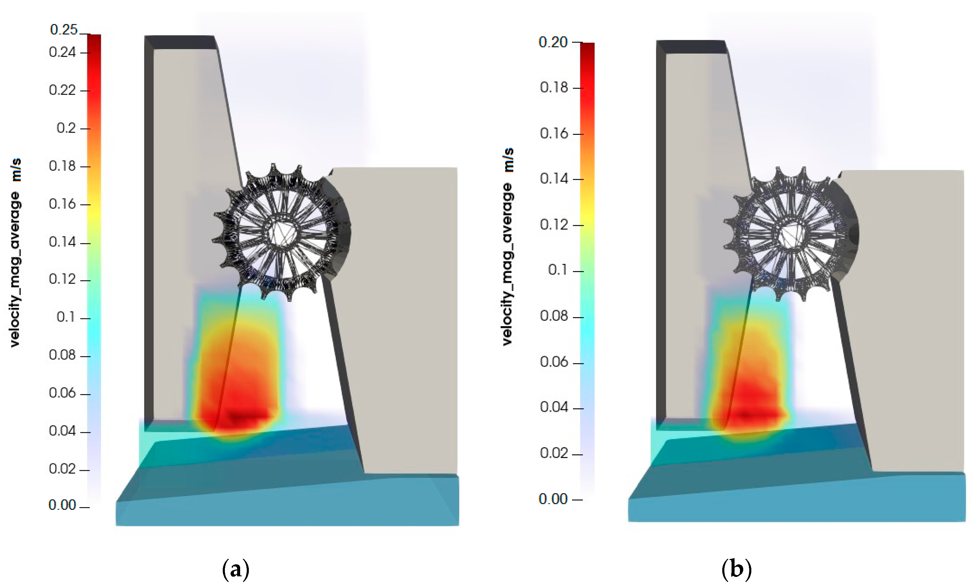
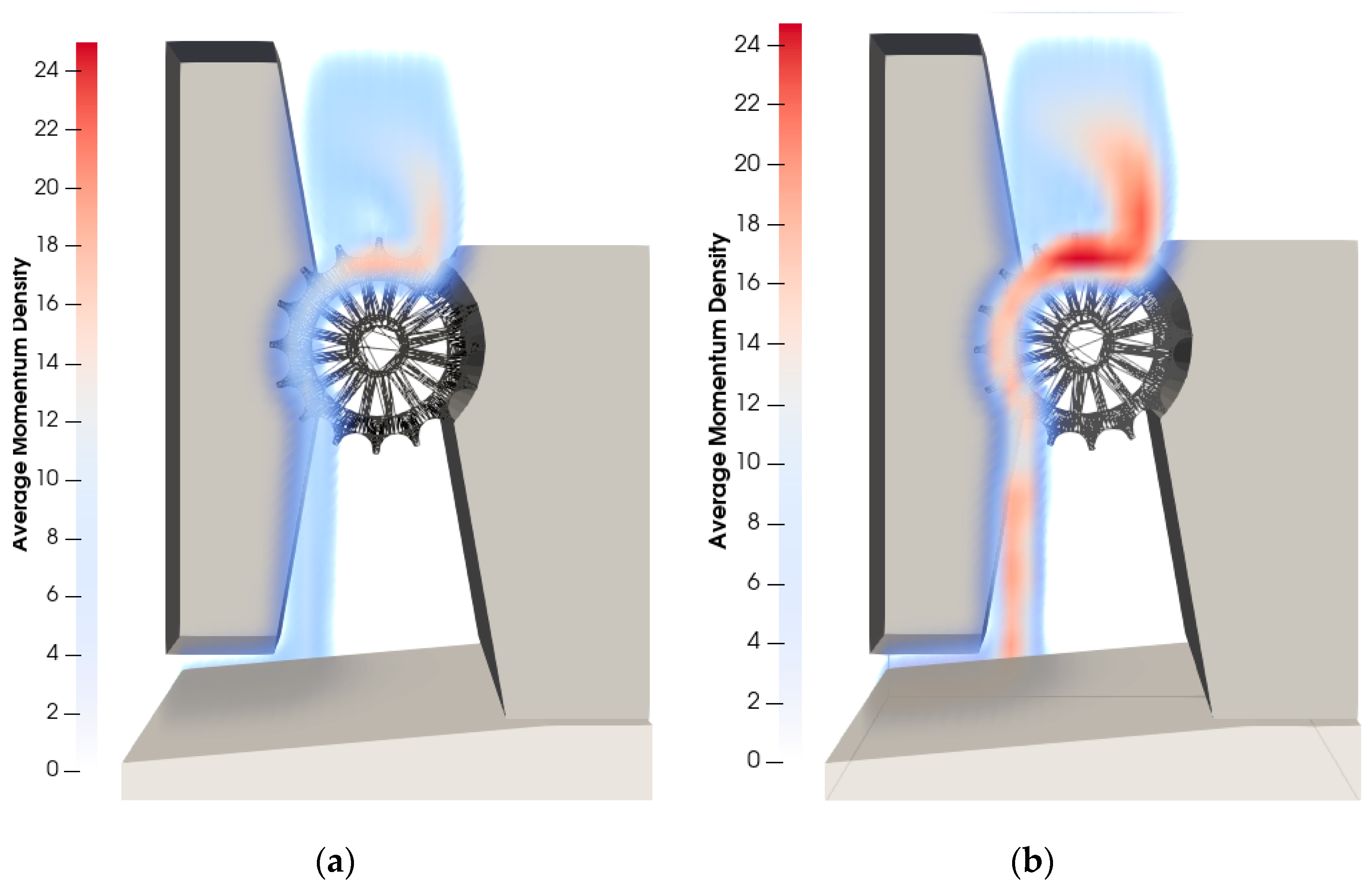
2.4. Continuum Transformations of the Discrete Element Data

While DEM data provide fundamental micromechanical insight into the behavior of bulk solids, they are also useful to understand important continuum quantities, such as the Cauchy stress tensor, the velocity field, the mass density field, and the momentum density. Such fields can be rigorously calculated via a coarse-graining approach, as proposed by Weinhart, et al. [19] and Goldhirsch [20] and further applied by Labra, et al. [21]. In this approach, a spatial-averaging function is used to compute continuum fields from discrete data in a series of points within a simulation domain. This implementation has been an initial version of the continuum analysis and EDEM 2020 has been used, while EDEM 2022 inlcudes a final built-in version of the analysis. The calculations in this work were performed following Goldhirsch (2010), as described in Equations (2)–(6):

$${\mathsf{\sigma }}_{\mathrm{c}}={{\displaystyle \sum }}_{\mathrm{i}}{\mathrm{b}}_{\mathrm{ij}}{\mathrm{F}}_{\mathrm{i}}\varphi \left(\mathrm{r}-{\mathrm{r}}_{\mathrm{i}}\right)$$

(2)

where ${\mathsf{\sigma }}_{\mathrm{c}}$ is the contact stress component of the Cauchy stress tensor, ${\mathrm{b}}_{\mathrm{ij}}$ is the contact branch vector, ${\mathrm{F}}_{\mathrm{i}}$ is the contact force tensor, and $\varphi$ is the Gaussian coarse-graining function.

$$\varphi \left(r\right)=\frac{1}{\sqrt{{\left(2\pi w\right)}^3}}{e}^{-\frac{{\left|r\right|}^2}{{\left(2w\right)}^2}}H\left(w-\left|r\right|\right)$$

(3)

where $H$ is the heavyside function, $w=3R$ is the coarse-graining width, and $R$ is the mean particle radius.

The microscopic mass density at point $r$ at time $t$ is defined in a continuum analysis, as follows:

$$\rho \left(r,t\right)={\displaystyle \sum }_i{m}_i\varphi \left(r-r_i\left(t\right)\right)$$

(4)

where $\rho$ is the mass density, and $m_i$ is the particle mass. Furthermore, the coarse-grained momentum density is defined by:

$$p\left(r,t\right)={\displaystyle \sum }_i{m}_i{v}_i\varphi \left(r-r_i\left(t\right)\right)$$

(5)

where p is the momentum density, and $m_i$ is the particle mass that corresponds to the equivalent microscopic momentum density field.

The coarse-grained velocity field is defined by:

$$V\left(r,t\right)=\frac{p\left(r,t\right)}{\rho \left(r,t\right)}$$

(6)

The EDEMPy library of functions was used to calculate the continuum fields in the analysis. It is a Python library for the postprocessing and analysis of EDEM simulation data that takes advantage of EDEM’s hdf5 file structure. A coarse-graining width of 3 times the mean particles was used in all the cases [21].

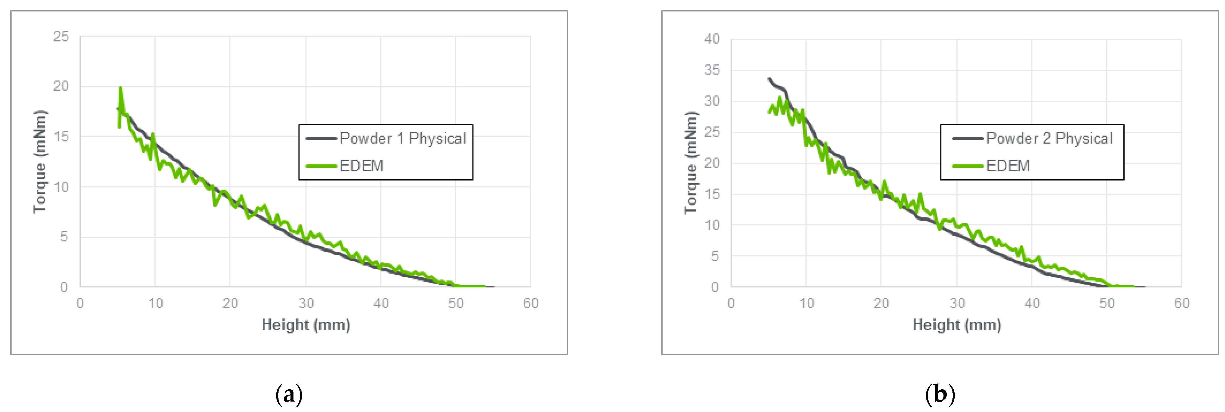
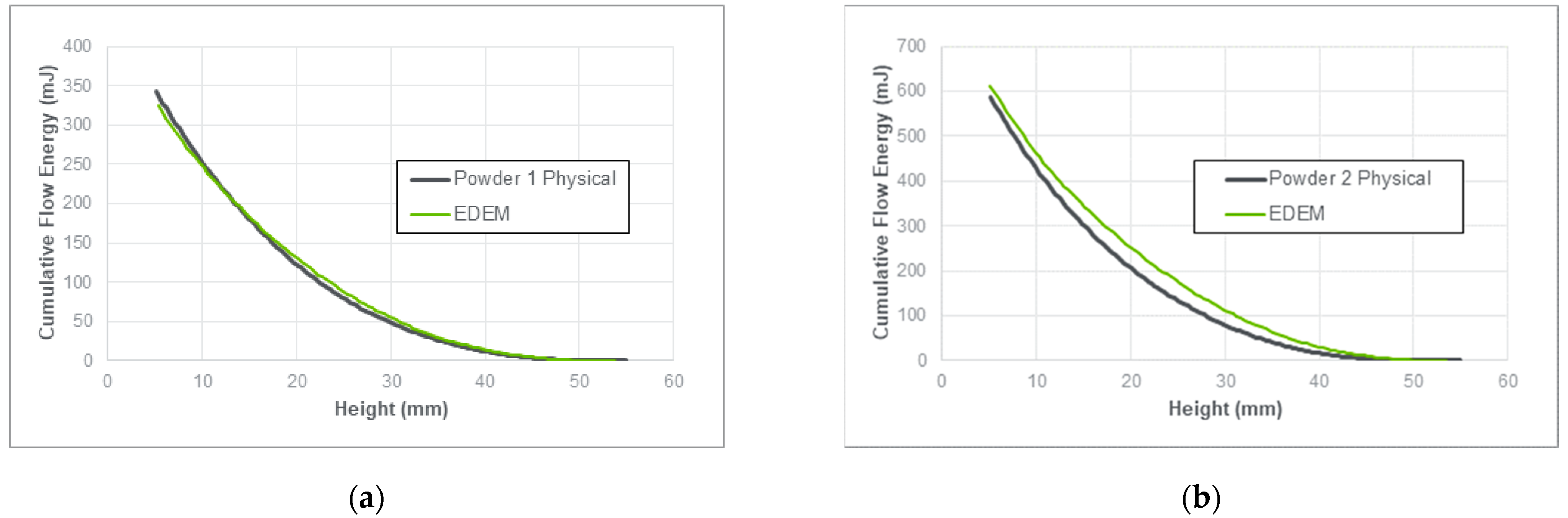
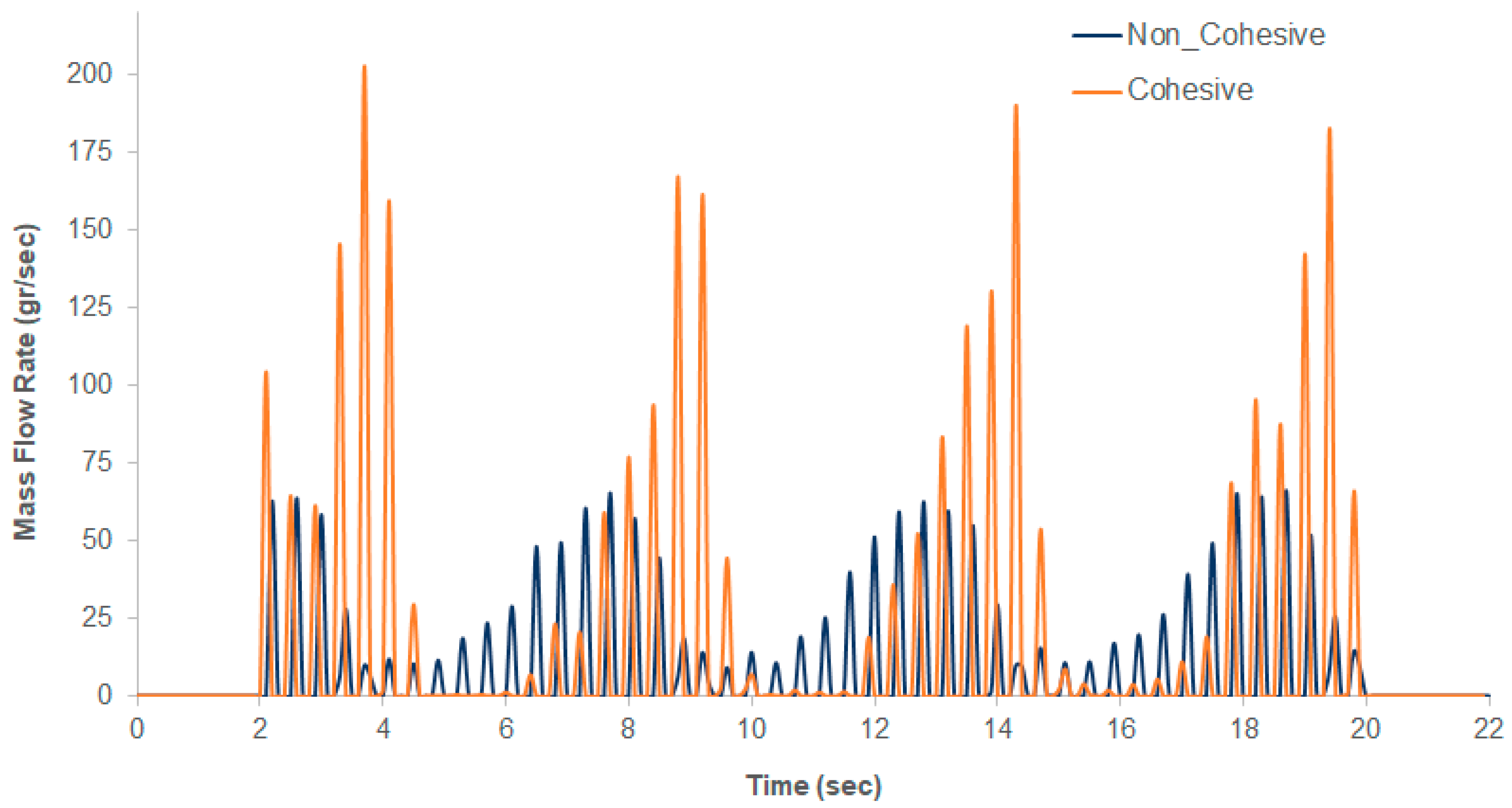
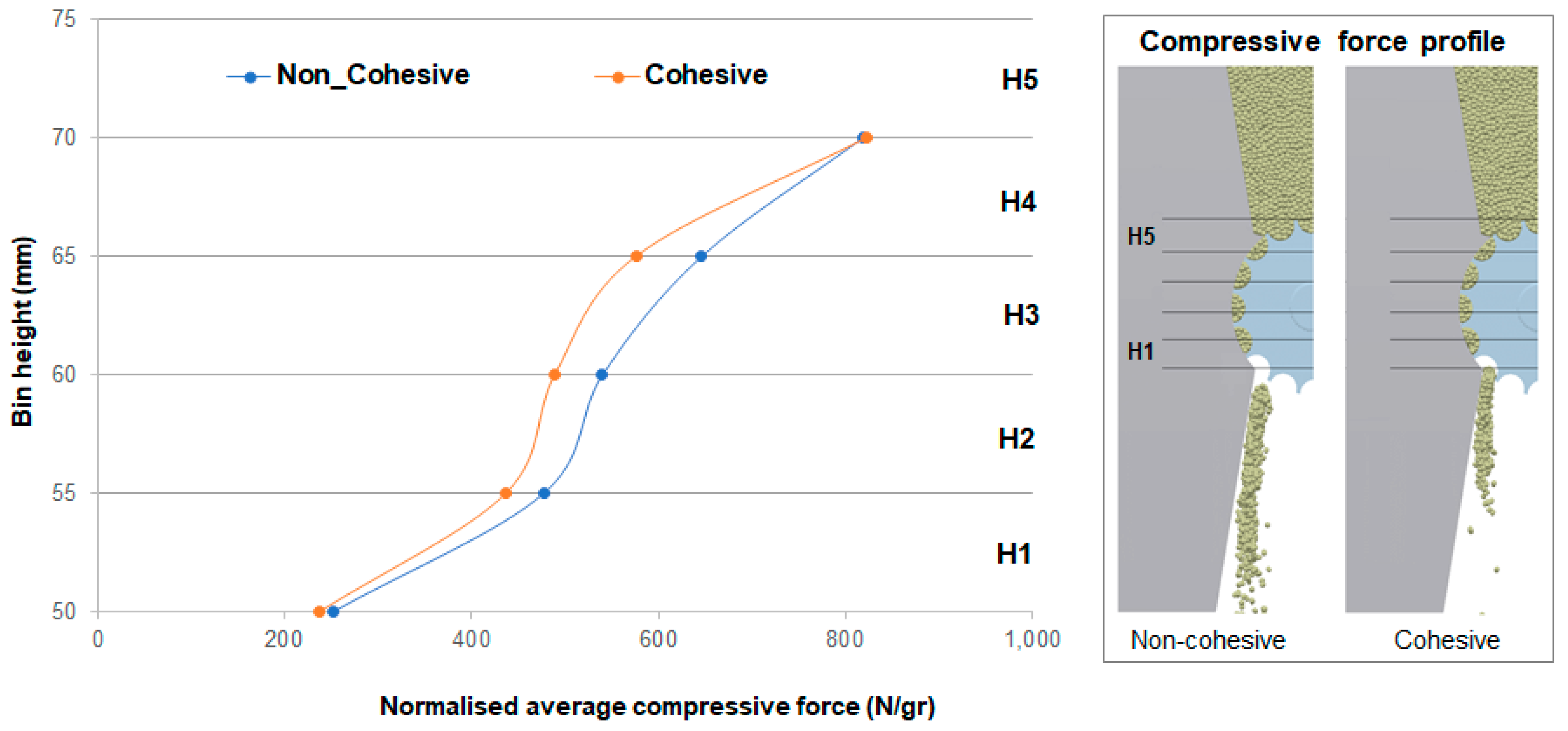
3. Results and Discussion

The following section includes results using EDEM 2020 with a customized initial version of the continuum analysis. Newer editions of EDEM include expanded built-in versions of the analysis. One of the main areas of interest was to investigate the effectiveness of the dose units. Thus, selected compartments (Bins 1–4) that encapsulated the dosing units were checked against the mass of material that was transferred (Figure 7). It was observed that, for both the cohesive and the free-flowing materials, the top dose unit (Bin 4) held the highest mass of material, followed by a progressive reduction in Bins 2 and 3, whereas the bottom unit (Bin 1) contained the lowest. It could also be observed that the highest reduction rate for both materials occurred in Bin 1, with the free-flowing material dropping by 26.6% and the cohesive material by 21.9%. The smaller reduction rate indicated that more particles were contained in the bottom unit, which could be attributed to the presence of cohesion and the creation of clusters.

Next, the profile of the mass flow rate is demonstrated in Figure 8. It could be observed that the cohesive material had abrupt releases of material with high peaks, whereas the profile of the free-flowing material appeared to be more uniform with lower peaks. This indicated the creation of agglomerates. This claim is verified by Figure 9, which shows the contact vectors between particles overlooking the top the area where the material landed. It could be observed that the cohesive material covered a much larger area compared to the free-flowing one.

To visualize the simulation data as a continuum, we computed the continuum physical quantities from the discrete data of EDEM using the methodlogy described by Labra, et al. [21], whereby distance-weighted averaging of the discrete data was performed around the nodes of a uniform, rectilinear grid of points in the domain using a Gaussian weighting function with a unity spatial integral. For this, EDEMPy was used, a Python library for the postprocessing and analysis of EDEM simulation data that takes advantage of EDEM’s hdf5 file structure. Figure 10 demonstrates the average velocities over time for the free-flowing and cohesive materials, respectively. It could be observed that the cohesive material had lower velocity during the entire simulation, and the shape of the velocity after exiting the wheel created a bottleneck. This indicated the presence of clusters, which is in good agreement with previous observations of agglomerate creation due to interparticle adhesion.

Furthermore, Figure 11 demonstrates the hydrostatic stress field, which is the first invariant of the Cauchy stress tensor. The results are presented as the average pressure over time for both materials. It could be observed that the cohesive material (b) was subjected into higher stresses, especially toward the top dose units. This was expected due to the presence of clusters and the increased contact between particles.

Next, Figure 12 shows the momentum density averaged over time for both the free-flowing and cohesive materials. The momentum density had units of kg/m²∙s and showed how much material was transferred. It could be observed that the cohesive material had a higher momentum density, which could be attributed to the fact that the agglomerates had stronger impacts with the surrounding walls, thus tending to break and create higher momentum density.

Further, investigating the profiles of the compressive forces in the region around the wheel (Figure 13), the height of the wheel was divided in equal horizontal layers, and the results were normalized against the masses of the particles for each material. It was observed that the profiles for both materials followed the same shape, but the cohesive material had an overall higher reduction rate at the H4 compartment than the free-flowing one. This indicated that the free-flowing material was better packed, which led to a more uniform force distribution.

4. Conclusions

In this paper, two powders of different flowability were modeled and calibrated against experimental testing. A complete and automated workflow was presented based on the previous work of the authors [6]. The results showed that the EDEM material models captured the complex micromechanical behavior of powders and provided excellent quantitative predictions of complex physical responses after calibration. The efficient model calibration methodology adopted in this work required only a small number of simulations, making the calibration of accurate models practical.

The calibrated material models were used to simulate an example of a dosing process for AM to better understand the mechanics of the system and the effect of powder properties on it. In addition, a coarse-grained approach was coupled with DEM to extract continuum fields from the discrete data.

The DEM was used to analyze in detail the mass flow and the effectiveness of the dose units against each material. It was observed that the presence of cohesion hindered the flow, as the dose units were filled with smaller amounts of material, while the flow at the outlet discharged the formed clusters, covering a larger area at the bottom of the equipment. Furthermore, the average velocity over time confirmed the creation of agglomerates for the cohesive material through the creation of bottleneck-shaped velocity compared with the free-flowing material. Finally, the average hydrostatic pressure and the compressive force profile were analyzed, highlighting the effect of cohesion on the mechanics of the system.

References

1. Frazier, W.E. Metal Additive Manufacturing: A Review. J. Mater. Eng. Perform. 2014, 23, 1917–1928. [Google Scholar] [CrossRef]
2. Guo, N.; Leu, M.C. Additive manufacturing: Technology, applications and research needs. Front. Mech. Eng. 2013, 8, 215–243. [Google Scholar] [CrossRef]
3. Gao, W.; Zhang, Y.; Ramanujan, D.; Ramani, K.; Chen, Y.; Williams, C.B.; Wang, C.C.L.; Shin, Y.C.; Zhang, S.; Zavattieri, P.D. The status, challenges, and future of additive manufacturing in engineering. Comput.-Aided Des. 2015, 69, 65–89. [Google Scholar] [CrossRef]
4. Mueller, B. Additive Manufacturing Technologies—Rapid Prototyping to Direct Digital Manufacturing. Assem. Autom. 2012, 32. [Google Scholar] [CrossRef]
5. Tumbleston, J.R.; Shirvanyants, D.; Ermoshkin, N.; Janusziewicz, R.; Johnson, A.R.; Kelly, D.; Chen, K.; Pinschmidt, R.; Rolland, J.P.; Ermoshkin, A.; et al. Continuous liquid interface production of 3D objects. Science 2015, 347, 1349–1352. [Google Scholar] [CrossRef]
6. Nan, W.; Pasha, M.; Bonakdar, T.; Lopez, A.; Zafar, U.; Nadimi, S.; Ghadiri, M. Jamming during particle spreading in additive manufacturing. Powder Technol. 2018, 338, 253–262. [Google Scholar] [CrossRef]
7. Yadroitsev, I.; Gusarov, A.; Yadroitsava, I.; Smurov, I. Single track formation in selective laser melting of metal powders. J. Mater. Processing Technol. 2010, 210, 1624–1631. [Google Scholar] [CrossRef]
8. Cundall, P.A.; Strack, O.D.L. A discrete numerical model for granular assemblies. Géotechnique 1979, 29, 47–65. [Google Scholar] [CrossRef]
9. Altair EDEM software, EDEM 2020.0 Documentation 2020. Available online: https://www.altair.com/edem/ (accessed on 2 August 2022).
10. Chung, Y.C.; Ooi, J.Y. Benchmark tests for verifying discrete element modelling codes at particle impact level. Granul. Matter 2011, 13, 643–656. [Google Scholar] [CrossRef]
11. Pantaleev, S.; Yordanova, S.; Janda, A.; Marigo, M.; Ooi, J.Y. An experimentally validated DEM study of powder mixing in a paddle blade mixer. Powder Technol. 2017, 311, 287–302. [Google Scholar] [CrossRef] [Green Version]
12. Bharadwaj, R.; Ketterhagen, W.R.; Hancock, B.C. Discrete element simulation study of a Freeman powder rheometer. Chem. Eng. Sci. 2010, 65, 5747–5756. [Google Scholar] [CrossRef]
13. Härtl, J.; Ooi, J.Y. Numerical investigation of particle shape and particle friction on limiting bulk friction in direct shear tests and comparison with experiments. Powder Technol. 2011, 212, 231–239. [Google Scholar] [CrossRef]
14. Luding, S. Cohesive, frictional powders: Contact models for tension. Granul. Matter 2008, 10, 235–246. [Google Scholar] [CrossRef]
15. Pasha, M.; Dogbe, S.; Hare, C.; Hassanpour, A.; Ghadiri, M. A new contact model for modelling of elastic-plastic-adhesive spheres in distinct element method. AIP Conf. Proc. 2013, 1542, 831–834. [Google Scholar]
16. Thakur, S.C.; Morrissey, J.P.; Sun, J.; Chen, J.F.; Ooi, J.Y. Micromechanical analysis of cohesive granular materials using the discrete element method with an adhesive elasto-plastic contact model. Granul. Matter 2014, 16, 383–400. [Google Scholar] [CrossRef]
17. Hare, C.; Zafar, U.; Ghadiri, M.; Freeman, T.; Clayton, J.; Murtagh, M.J. Analysis of the dynamics of the FT4 powder rheometer. Powder Technol. 2015, 285, 123–127. [Google Scholar] [CrossRef]
18. Sousani, M. Calibrating DEM Models for Powder Simulation: Challenges, Advances & Guidelines; Altair-Engineering Ltd.: Edinburgh, UK, 2019. [Google Scholar]
19. Weinhart, T.; Labra, C.; Luding, S.; Ooi, J.Y. Influence of coarse-graining parameters on the analysis of DEM simulations of silo flow. Powder Technol. 2016, 293, 138–148. [Google Scholar] [CrossRef]
20. Goldhirsch, I. Stress, stress asymmetry and couple stress: From discrete particles to continuous fields. Granul. Matter 2010, 12, 239–252. [Google Scholar] [CrossRef]
21. Labra, C.; Ooi, J.Y.; Sun, J. Spatial and temporal coarse-graining for DEM analysis. AIP Conf. Proc. 2013, 1542, 1258–1261. [Google Scholar]
Figure 1. Bi-sphered particle with an aspect ratio of 1.25 used in the DEM simulations.
Processes 10 01754 g001
Figure 2. Schematic representation of the FT4 test used for material characterization [18].
Processes 10 01754 g002
Figure 3. Cross-sections of the DEM model replicating the FT4 rheometer basic flow energy test and demonstrating the different stages of the procedure.
Processes 10 01754 g003
Figure 4. Experimental and simulated torques on the impeller blade during the basic flow energy test cycle at 100 mm/s blade-tip speed for (a) free-flowing powder and (b) cohesive powder.
Processes 10 01754 g004
Figure 5. Experimental and basic flow energies at 100 mm/s blade-tip speed for (a) free-flowing powder and (b) cohesive powder.
Processes 10 01754 g005
Figure 6. Schematic of the virtual dosing wheel equipment used in the DEM simulations.
Processes 10 01754 g006
Figure 7. Schematic of the dosing wheel showing the calculated amounts of mass per dose unit for each powder material, as well as their reduction rates.
Processes 10 01754 g007
Figure 8. Mass flow rate for the free-flowing (blue) and the cohesive (orange) materials.
Processes 10 01754 g008
Figure 9. Top view and zoomed-in areas of the ground floor, highlighting the contact vectors between particles.
Processes 10 01754 g009
Figure 10. Average velocities over time for (a) the noncohesive and (b) cohesive materials.
Processes 10 01754 g010
Figure 11. Average hydrostatic pressures over time for (a) the noncohesive and (b) cohesive materials.
Processes 10 01754 g011
Figure 12. Average momentum density (kg/m2∙s) for the (a) free-flowing and (b) cohesive materials.
Processes 10 01754 g012
Figure 13. Profile of the average compressive force normalized against the mass of each particle covering the vertical height of the wheel for the free-flowing (blue) and the cohesive (orange) materials.
Processes 10 01754 g013