

Numerical Study for Flow Loss Characteristic of an Axial-Flow Pump as Turbine via Entropy Production Analysis
by
Fan Yang
1,2,3,*,
Zhongbin Li
1,
Yiping Cai
4,
Dongjin Jiang
1,
Fangping Tang
1,3 and
Shengjie Sun
1 1
College of Hydraulic Science and Engineering, Yangzhou University, Yangzhou 225009, China
2
Jiangxi Research Center on Hydraulic Structures, Jiangxi Academy of Water Science and Engineering, Nanchang 330029, China
3
Hydrodynamic Engineering Laboratory of Jiangsu Province, Yangzhou 225009, China
4
Water Resources Research Institute of Jiangsu Province, Nanjing 210017, China
*
Author to whom correspondence should be addressed.
Processes 2022, 10(9), 1695; https://doi.org/10.3390/pr10091695
Submission received: 23 July 2022
/
Revised: 21 August 2022
/
Accepted: 22 August 2022
/
Published: 26 August 2022
(This article belongs to the Topic Latest Developments in Fluid Mechanics and Energy)
Abstract
:Low-head vertical axial-flow pump as turbine (PAT) devices play a vital part in the development of clean energy for hydropower in plain areas. The traditional method of evaluating the flow loss in hydraulic machinery is calculated by the pressure drop method, the limitation of which is that the location of the occurrence of large losses cannot be accurately determined. In this paper, entropy production theory is introduced to evaluate the irreversible losses in the axial-flow PAT from the perspective of the second law of thermodynamics. A three-dimensional model of the axial-flow PAT is established and solved numerically using the Reynolds time-averaged equation, and the turbulence model is adopted as Shear Stress Transport–Curvature Correction (SST-CC) model. The validity of the entropy production theory to evaluate the energy loss distribution of the axial-flow PAT is illustrated by comparing the flow loss calculated by the pressure drop and the entropy production theory, respectively. The entropy production by turbulent dissipative dominates the total entropy production in the whole flow conduit, and the turbulent dissipative entropy accounts for the smallest percentage of the whole conduit entropy production at the optimal working condition Qbep, which is 51%. The impeller and the dustpan-shaped conduit are the essential sources of hydraulic loss in the entire flow conduit of the axial-flow PAT, and most of the energy loss of the impeller occurs at the blade leading edge, the trailing edge, and the flow separation zone near the suction surface. The energy loss of the dustpan-shaped conduit results from the high-speed flow from the impeller outlet to dustpan-shaped conduit to form a vortex, backflow and other chaotic flow patterns. Flow impact, flow separation, vortex and backflow are the main causes of high entropy production and energy loss.
1. Introduction
With the global energy shortage, climate change and people’s awareness of eco-environmental protection, accelerating the development of renewable energy to ensure the safety of the ecological environment has become the focus of attention of all countries in the world. China has proposed to achieve peak carbon emissions and carbon neutral status by 2030 and 2060, respectively [1], and plans to increase the proportion of non-fossil energy generation to 39% by 2025. In terms of China’s power generation structure in 2021, thermal power generation in the country still dominates, with 577,027 million kWh of thermal power generation, accounting for 71.13%, while hydro power generation is second, with 118,420 million kWh of power generation, accounting for 14.60% [2]. Hydroelectric energy is the second largest energy source in China after coal, and it is also the clean energy source that can form the largest supply scale among renewable energy sources. Meanwhile, China is rich in hydropower resources [3], and the development of hydropower is in line with China’s renewable energy development strategy, which plays an important role in alleviating environmental and energy problems. Thanks to the abundant hydro energy resources and national energy development policies, hydropower generation has a very broad potential and prospect.
Unlike the topographic restrictions and high head difference requirements for building high-head turbines, small- and medium-sized PATs have more application scenarios in plain areas [4,5]. Meanwhile, with the rapid development of technology and the widespread use of PATs, scholars have conducted lots of research on the internal flow characteristics of PATs [6,7,8]. Liu et al. [9] predicted the hump characteristics of a PAT using the SST k-ω model based on the compressible cavitation model. The results agreed well with the experimental data and found that the hump characteristics may be associated with the cavitation phenomenon on the suction side of the flow channel, while the rotational speed is a key factor leading to pressure fluctuations when cavitation is severely. Ran et al. [10] measured the pressure pulsation at the unstable operating point to obtain the energy performance of a model PAT, and thus, they analyzed the operating instability in the PAT at most flow rate conditions. Li et al. [11] conducted numerical simulations to analyze the hydraulic transient pressure fluctuations and flow behavior of the prototype PAT during normal shutdown. It was found that when the guide vane is closed, both flow rate and runner torque decrease, and the rotational speed decreases due to the negative torque that appears on the runner. The transient characteristics during shutdown were accurately predicted, and the internal flow behavior of the PAT was revealed. Kim et al. [12] applied the SAS-SST model for 3D unsteady RANS to numerically verify the transient pressure and vortex rope variation patterns obtained from model tests and elucidated the internal flow and unsteady pressure phenomena of the model pump turbine at various Thoma numbers. At present, some scholars have focused on testing the effects of different runner geometry parameters on the hydraulic performance and operational stability of PATs so as to improve the optimal design of PAT. Olimstad et al. [13] tested the effects of different inlet blade angle and radius of curvature of runners on the reversible pump-turbine energy performance by experiments and numerical simulations. The results indicated that the smaller inlet blade angle resulted in less steep characteristic of the performance curve in turbine mode, while the S-zone measured in turbine braking and pump operating modes became more exaggerated. Liu et al. [14] investigated the pressure pulsation characteristics and leakage vortex intensity of a mixed-flow PAT under different blade tip clearances and proposed the classification of blade tip leakage vortex and the main influencing factors of leakage vortex intensity. Yang et al. [15] found that the shortening of the impeller blade passage and the reduction in the velocity gradient were the reasons for the reduction in the hydraulic loss in the impeller by detailed analysis of the distribution of the hydraulic loss of PAT at different blade wrap angles.
Reducing the energy loss of PAT is essential to improve the performance of hydroelectric power plants. Traditional pressure drop method for calculating losses cannot locate the magnitude and location of losses visually and specifically, and the link between flow instability and energy loss has not been revealed quantitatively [16,17,18]. To overcome the limitations of the pressure drop method, the entropy production theory based on the second law of thermodynamics was introduced to evaluate the hydraulic losses within fluid machinery. Kock [19] proposed the formulation of entropy production for complex turbulent viscous flow and its use in CFD back in 2005. However, the method proposed by Kock and Herwig [20,21] could not accurately capture the entropy production in the near-wall region because of the significant velocity gradient generated by the fluid viscosity in the near-wall laminar boundary layer. Duan et al. [22,23] proposed a wall equation using wall shear stress and velocity to obtain entropy production near the wall. Nowadays, numerical prediction methods of entropy production theory have a very wide applicability in the industrial field. More and more scholars have introduced entropy production theory to analyze the flow losses within fluid machinery. Gong et al. [24] successfully applied entropy production theory to acquire the performance of a hydraulic turbine and clarified the magnitude and distribution location law of energy dissipation within the flow channel. Silva-llanca [25] evaluated the efficiency of different strategies to cool data center rooms via entropy production theory analysis. Ries [26] used direct numerical simulation (DNS) to analyze the near-wall heat transport processes and entropy production mechanisms in turbulent jets. In addition, entropy production theory plays a guiding role in the PAT design optimization. Hou et al. [27] applied entropy production theory to optimize the design of an ultra-low specific speed centrifugal pump for a combination of several parameters and obtained the optimal solution after optimization analysis, indicating that pump optimization with minimum local entropy production rate as an indicator is feasible. Ji et al. [28] explored the influence of different impeller tip clearances on the internal flow field and hydraulic losses of a mixed-flow pump using entropy production theory and found that the impeller hydraulic loss and total entropy production increased significantly when the impeller tip clearance increased, and it was vital to select the proper size of the impeller tip clearance while considering the overall performance of the device. In hydraulic machinery, cavitation flow is often generated when the local pressure is lower than the saturation pressure [29], and the location of cavitation occurrence is often located on the blade surface or in draft tube, which is prone to local performance degradation and unstable flow patterns [30,31]. Wang et al. [32] developed an entropy production diagnostic model (EPDM) with phase transition (EPDMS) to analyze the irreversible loss of cavitation flow in fluid machinery. Lai et al. [33] used a modified Zwart cavitation model to simulate the cavitation flow in a centrifugal pump in order to reveal the reason for the sharp decrease in cavitation flow head in the experiment. It was found that the sharp decrease in cavitation flow head was associated with the rapid increase in entropy production near the impeller pressure side and the impeller blade trailing edge. Zhao et al. [34] studied the cavitation flow inside a slanted axial-flow pump based on the entropy production theory and vortex dynamics, where the impeller is the main part of the loss occurring in cavitation. He revealed the loss of energy and entropy production rate in the incipient, growing and wedge cavitation stages.
In conclusion, entropy production theory has wide applicability, and previous studies have focused on the performance optimization and flow field analysis of pumps, turbines, but there are still relatively few studies that apply entropy production theory to analyze a low-head axial-flow PAT. From previous studies, we know that the hydraulic losses in fluid machinery are mainly associated with undesirable flow regimes such as flow impact, blade wake, flow separation, cavitation flow [35] and vortices [36]. The detailed location of the occurrence of these losses still needs to be determined.
In this paper, the hydraulic losses in turbine mode of the axial-flow PAT were analyzed at different flow conditions via the entropy production theory method. The hydraulic loss calculated by entropy production and pressure drop are compared, indicating that the entropy production theory is reliable for evaluating the energy loss characteristics in the axial-flow PAT. The variation of total entropy production and entropy production proportion of different components with flow rate was quantitatively analyzed. The magnitude and distribution characteristics of the detailed local entropy production rate of the main parts (impeller, guide vane and dustpan-shaped conduit) of the axial-flow PAT where energy dissipation occurs are located. Additionally, the distribution of the high entropy production region and the causes of energy loss in the axial-flow PAT are clarified.
2. Entropy Production Theory
Entropy is a thermodynamic state parameter of matter that is used to describe the degree of disorder in a system. In accordance with the second law of thermodynamics, an actual fluid system is always accompanied by entropy production during operation. Because of the large specific heat capacity of water, the flow inside the PAT can be considered as constant temperature flow, i.e., the temperature is assumed to be constant in the calculation process. Due to the viscosity of water and Reynolds stress, there are energy dissipation in the flow process caused by irreversible factors, the viscous force of the fluid will transform kinetic and pressure energy into internal energy and dissipation. In addition, the internal vortex, backflow and other unstable flow phenomena in the flow field will lead to an increase in entropy production, accompanied by an increase in hydraulic losses. Hence, the hydraulic loss within the PAT can be evaluated by entropy production method.
In the mainstream region with high Reynolds number, the unsteady turbulent motion causes the loss of head and the increase in entropy. When the RANS turbulence model is applied for calculation, some variables in the turbulent flow are averaged, and the real velocity of the fluid mass consists of the average velocity and the pulsation velocity. Therefore, the entropy production also contains two parts, which are the entropy production caused by the time-averaged motion and the entropy production generated by the turbulent energy dissipation caused by the pulsation velocity. Herwig and Kock et al. [19,20,37] adopted the Reynolds time-averaged method to derive the entropy production rate per unit volume and gave a model for calculating the entropy production rate of the time-averaged flow field and the pulsating flow field.
The entropy production rate by direct dissipative (EPDD) resulting from the time-averaged motion is calculated as follows:
The entropy production rate by turbulent dissipation (EPTD) due to velocity fluctuation is calculated as follows:
where is the effective dynamic viscosity, (Pa·s); is the turbulent viscosity; and is the turbulent dynamic viscosity.
The entropy production induced by time-averaged motion can be obtained directly from the calculation results, while for the entropy production induced by velocity fluctuation, it generally needs to be corrected according to the turbulence equation. The turbulent velocity fluctuation is related to ε and ω in the turbulent model [21,38]. When the Reynolds number is large, the entropy production induced by velocity fluctuation in the SST k-ω model can be calculated by the following equation:
where ; is the turbulent eddy frequency, s−1; and is the turbulent kinetic energy, m2/s2.
The local entropy production rate (LEPR) can be expressed as:
In recent years, scholars have found that different from flow characteristics in mainstream region, a large velocity gradient is generated near the wall due to the viscous effect of the flow, and there is a strong wall effect on the entropy production. Kock and Herwig [20,21] found that the entropy production calculated by DNS and RANS methods was different, and the entropy production near the wall region were much larger than other area, so the hydraulic loss calculated by the entropy production method was much higher than that calculated by pressure drop method. Duan [22,23] proposed to use the wall shear stress and the velocity near the wall to calculate the entropy production rate by wall shear (EPWS):
where is the wall shear stress, Pa; and is the velocity at the center of the first layer of the grid near the wall, m/s.
The entropy production in the mainstream region can be calculated by volume integration of the entropy production rate induced by time-averaged velocity and velocity fluctuation, and the entropy production by wall shear can be obtained by area integration of the entropy production rate near the wall region:
The total entropy production of each region can be expressed as:
where is the entropy production induced by the time-averaged velocity; is the entropy production induced by the velocity fluctuation; is the entropy production by wall shear; V is the volume of fluid domain; and A is the wall area of fluid domain.
For the incompressible flow in the axial-flow PAT, the irreversible energy loss arises due to the viscous dissipation of the flow when the temperature change in the flow field is ignored, then the hydraulic loss in the flow field calculated by entropy production can be expressed as [39]:
where is the temperature of the flow field, is the total entropy production, and is the mass flow rate of the unit.
3. Experimental Model and Numerical Simulation Methods
3.1. Geometric Model
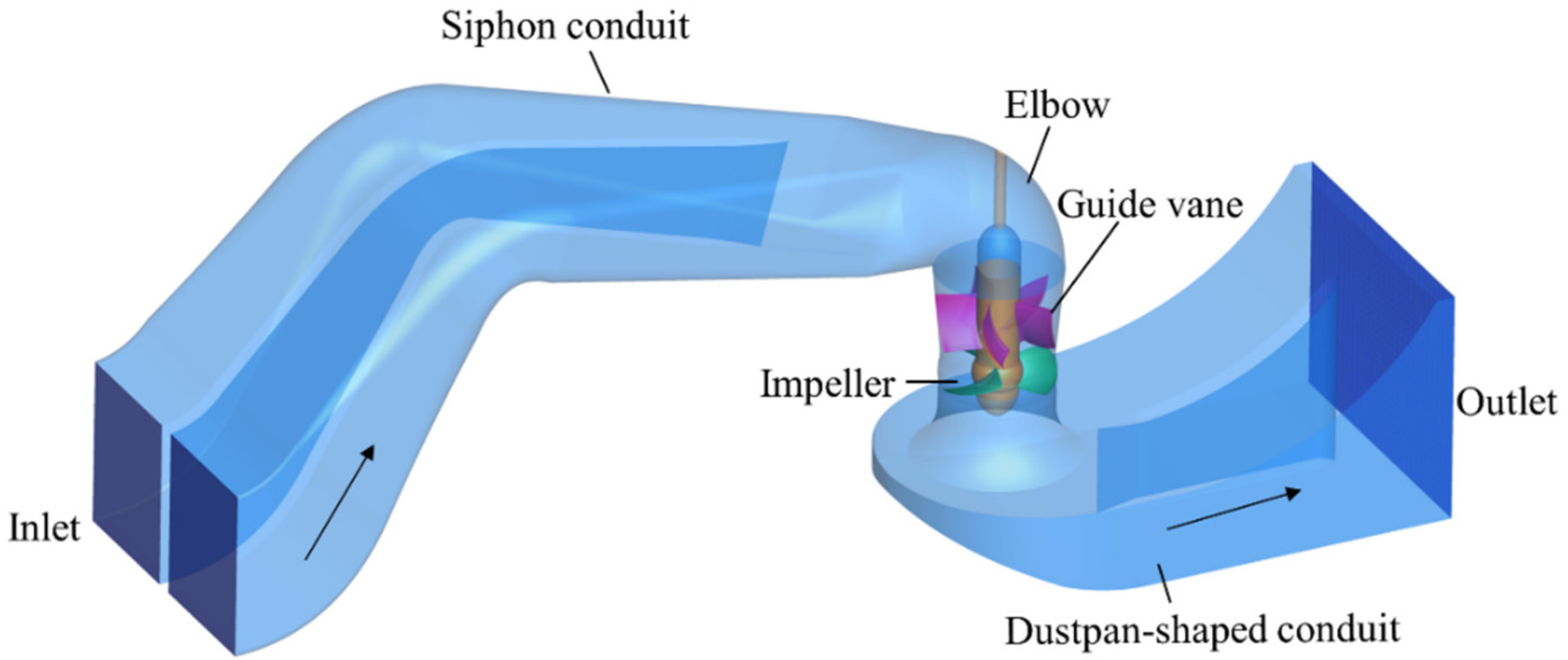
As shown in Figure 1, the object of this study is a vertical axial-flow PAT with a siphon conduit, a dustpan-shaped conduit, an impeller and a guide vane body. UG NX modeling software is used to build a three-dimensional model of the vertical axial-flow PAT. The main parameters are: nominal impeller diameter 300 mm, number of impeller blades 3, number of guide vanes 5, tip clearance 0.2 mm, optimal working flow rate, head, and rated speed 272 L/s, 2.4 m and 930 rpm, respectively. Geometric parameters of the dustpan-shaped conduit and siphon conduit can be found in reference [40].
3.2. Physical Model and Test
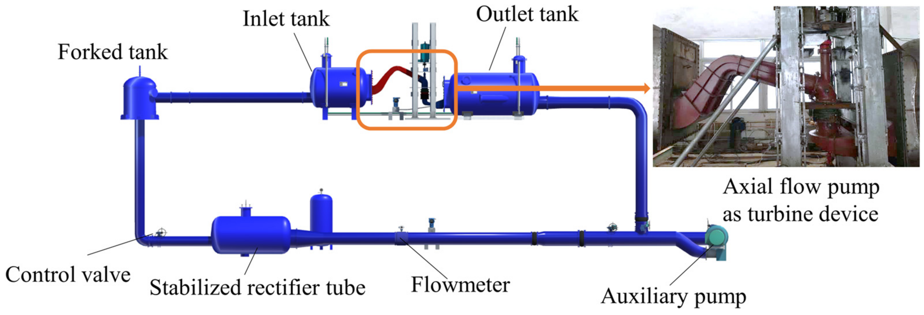
Figure 2 shows the test bench and model device of the axial-flow PAT. The test bench is a vertical closed-loop system. The differential pressure transmitter EJA110A with ±0.18% test error is used for head measurement, which is obtained by measuring the total pressure difference between the two pressure measuring sections of the inlet and outlet of the pump device. The E-mag type DN400 electromagnetic flow meter with ±0.015% test error is used for flow measurement. The ZJ 500 type speed and torque sensor is used for speed and torque measurement, and the test error of ZJ 500 speed and torque sensor in measuring speed and torque is ±0.24% and ±0.05%, respectively. The system uncertainty and random uncertainty of the performance efficiency of the vertical axial-flow PAT test bench were measured and calculated, and the comprehensive uncertainty of the test bench was obtained as ±0.368%. The comprehensive uncertainty of the test bench meets the accuracy requirement of the experiment. The head and efficiency of the axial-flow PAT were measured at the rated speed of 930 rpm for different flow conditions to acquire the performance curve.
3.3. Numerical Simulation Methods
3.3.1. Control Equations
The fluid inside the vertical axial-flow PAT is approximated as incompressible three-dimensional viscous turbulent flow, without considering the small temperature change during the experiment, and the water flow temperature is 25 °C. The continuity and the Navier–Stoker (RANS) equations (Equations (10) and (11)) were solved to simulate the internal flow of the vertical axial-flow PAT.
where , are the velocity components of the fluid in the i, j directions, respectively; is the time; is the density of the water; , is the component of the spatial coordinate; and is the hydrodynamic viscosity.
3.3.2. Turbulence Model
Menter [41] proposed the Shear Stress Transport k-ω (SST k-ω) model based on Wilcox [42] to address the problem that the Wilcox k-ω model is extremely sensitive to the ω value of the free incoming flow. SST k-ω model combines Wilcox k-ω model and standard k-ε model through a hybrid function. After dealing near-wall region with Wilcox k-ω model and dealing mainstream region with standard k-ε model, SST k-ω model successfully exploiting the advantages of both models while overcoming disadvantage of Wilcox k-ω model. SST k-ω model takes the effect of turbulent shear stress transport in the adverse pressure boundary layer into consideration, which leads to the good effect in predicting flow separation points and separation zones under pressure gradient conditions. The equations of the SST k-ω model are as follows:
where , , , , , , and .
A rotation correction function (Equation (17)) was proposed by Spalart and Shur [43] to solve the problem that eddy viscosity model is difficult to capture strong rotation and large curvature flow. The rotation and curvature correction method was introduced in the Spalart–Allmaras (SA) model of one equation at the first time. Smirnov and Menter [23] modified the SST k-ω model of the two equations to form the Shear Stress Transport–Curvature Correction (SST-CC) model considering rotation and curvature correction. It turns out that SST-CC model can recognize the stabilization effect of the rotation near the vortex axis, which strongly suppresses the vortex viscosity in this region. As the numerical requirement between SST model and SA model is different, the SST-CC model is restricted with a rotation function (Equation (25)). The SST-CC model has achieved good application effect in the prediction of the external characteristics of the rotating machinery and the three-dimensional turbulent field [44,45,46]. In this paper, the SST-CC turbulence model is chosen for the simulations.
where the constants , and are 1.0, 2.0 and 1.0, respectively; and and are related to the strain rate tensor and the rotation rate tensor :
where is 0 when there is no system rotation, is the Lagrange derivative of the strain tensor, and is the turbulent frequency.
The generating term Pk of the k and ω transport equations in the SST model is modified to Pk·fr.
where the scale factor is 1.
3.3.3. Mesh Generation
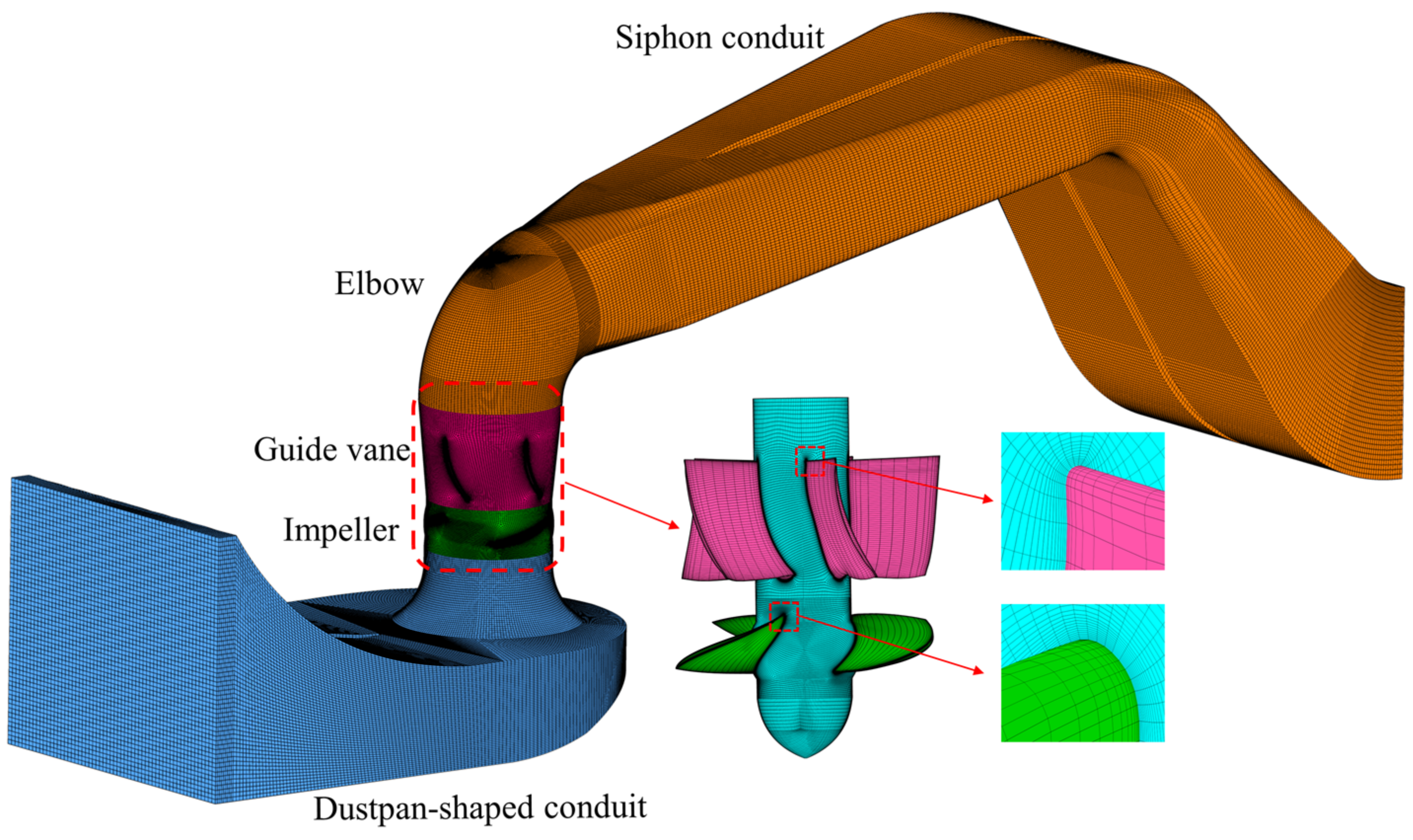
As shown in Figure 3, the axial-flow PAT computational domain is divided into five parts, namely, the siphon conduit, the elbow, the guide vane, the impeller and the dustpan-shaped conduit. The ICEM CFD software is applied for hexahedral meshing of the axial-flow PAT computational domain. Because the mesh quality has a great influence on the accuracy of numerical simulation results, the Jacobian value of each computational domain is controlled to be greater than 0.6. Local mesh refinement is carried out on the root of the impeller and guide vane. The automatic wall function is used to process the turbulent flow in the near-wall region. The dimensionless distance from the center of the first-layer grid in the near-wall region to the wall y+ is less than 30 in the impeller domain.
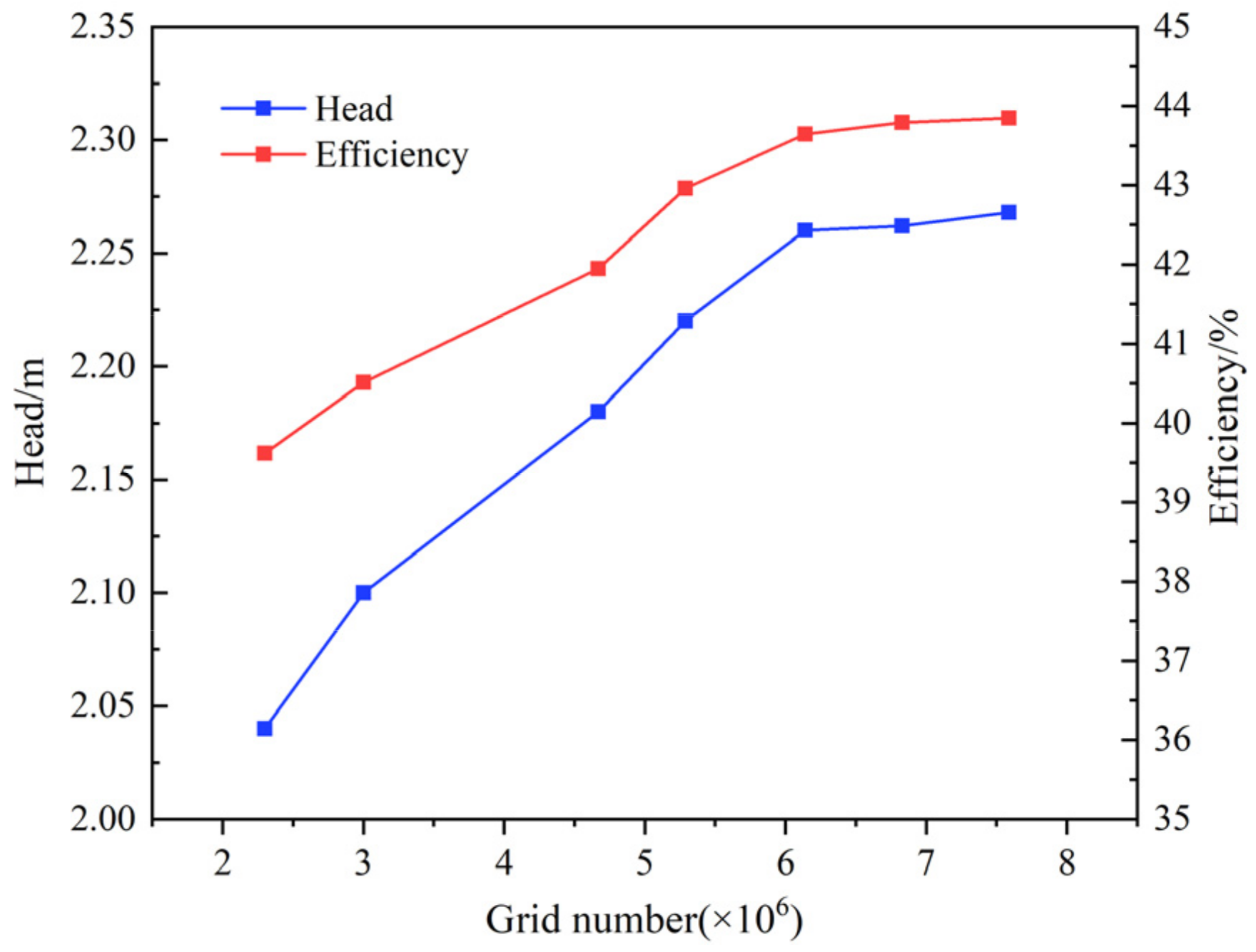
In numerical simulation, it is necessary to verify the independence of the grid number, the purpose of which is to reduce the influence of grid number and size on the calculation results. When the grid is refined to a certain extent, the solution result will not change significantly with the change in the grid number so that the sensitivity of the solution result to the mesh number is reduced. Under the optimal working condition (1.0Qbep), the efficiency and head of pump device with different grid numbers are analyzed for grid number independence. A total of 7 schemes of grids are used to verify the grid number independence, as shown in Figure 4. When the number of grids reaches 6.14 million, the change speed of the pump head and efficiency slows down significantly, and the relative deviation is less than 0.5%, which meets the stability requirements of the calculation. Considering the calculation accuracy and computational resource, the scheme with a total number of grids of about 6.14 million is suitable for this simulation.
Roache [47] proposed the Grid Convergence Index (GCI) to calculate the discrete error and judge the grid convergence error. GCI is currently the most reliable and widely used method to predict the numerical simulation uncertainty. The detail GCI calculation steps refers to Celik et al. [48]. Three groups of grids N1 = 6,143,640, N2 = 2,746,492 and N3 = 721,326 are selected for grid convergence analysis, and the axial-flow PAT efficiency is used as the grid error evaluation variable Φ. The calculation results of grid error are shown in Table 1. The optimal grid index GCI21 is 1.13%, which satisfies the convergence criterion. Therefore, the final grid number in the numerical simulation is 6,143,640.
3.3.4. Boundary Conditions
The flow in the axial-flow PAT is a three-dimensional incompressible complex turbulent motion, and the commercial software ANSYS CFX based on finite volume method is used to predict the complex flow in the flow conduit. The dynamic and static interface on both sides of the impeller is set to Stage, and the static and static interface is set to None. The general grid interface (GGI) is used to connect the grids of adjacent computing domains. GGI has strong adaptability in data transmission and connect different types of grids on both sides of the interface. The inlet boundary condition is set to mass flow and the outlet is set to static pressure. The wall in the entire conduit is set as non-slip wall. The calculated convergence accuracy is set to 10−5.
4. Results and Discussion
4.1. Comparison of Test and Simulation Performance Curves
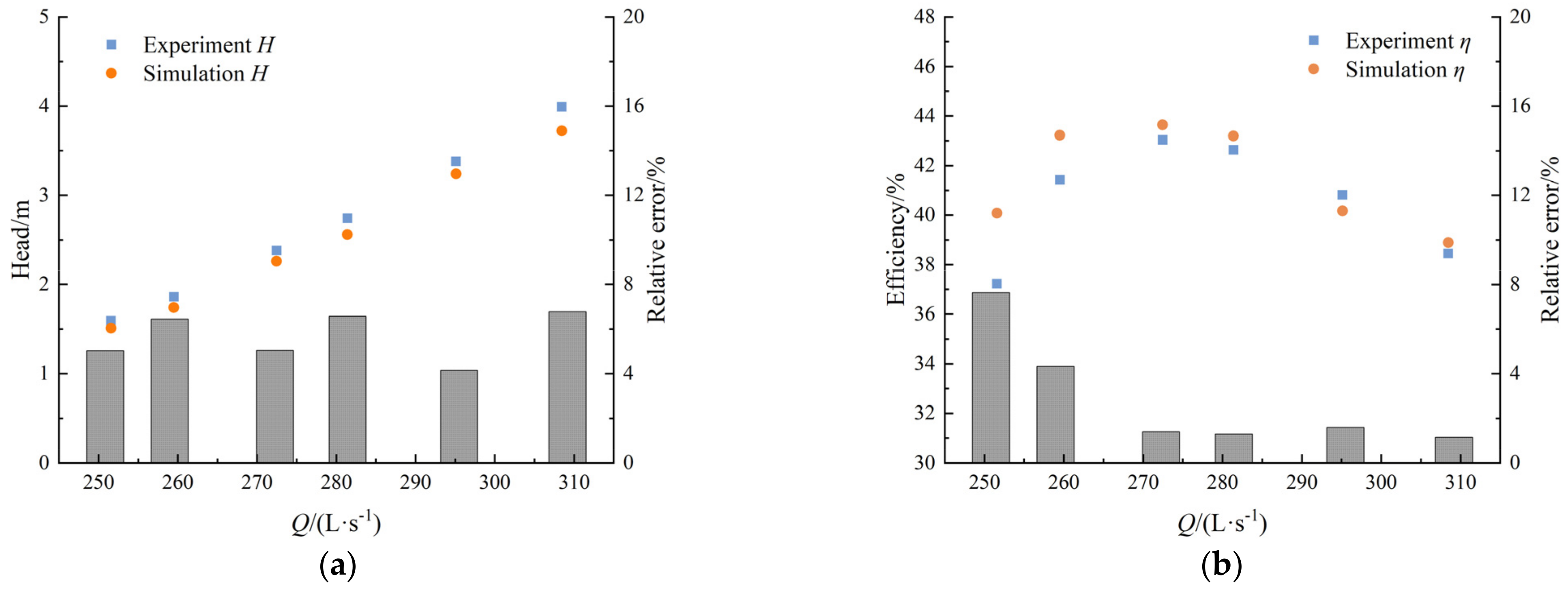
Figure 5 displays the comparison of hydraulic characteristics between simulation and experiment of the axial-flow PAT. Obviously, the performance curve of the simulation is in good consonance with the curve acquired by the experimental test. As the flow rate changes, the relative error between the experimental and the numerical simulation results is maintained in a relatively small fluctuation range. As shown in Figure 5a, the maximum head relative error is 6.8%. In Figure 5b, the maximum efficiency relative error of the numerical calculation and the model test is 7.63% at the small flow rate. Near the optimal flow rate, the efficiency relative error is 1.40%. In this paper, the reliability of numerical calculation results is verified.
4.2. Comparison of Hydraulic Loss Calculated by Entropy Production and Pressure Drop
In hydraulic machinery, the hydraulic loss in the whole domain is traditionally obtained by calculating the pressure drop between the inlet and outlet of each domain. In the axial-flow PAT, the static domains such as the siphon conduit, the elbow, the guide vane and the dustpan-shaped conduit are calculated by Equation (27). The impeller is the rotating domain and the hydraulic loss is calculated by the total rotating input work minus the work obtained by the increase in the liquid pressure, which is calculated by Equation (28).
where is the hydraulic loss obtained by the pressure difference between the inlet and the outlet; , is the total pressure of the inlet and outlet sections, respectively; is the mass flow of the axial-flow PAT; and is the input power of the pump shaft.
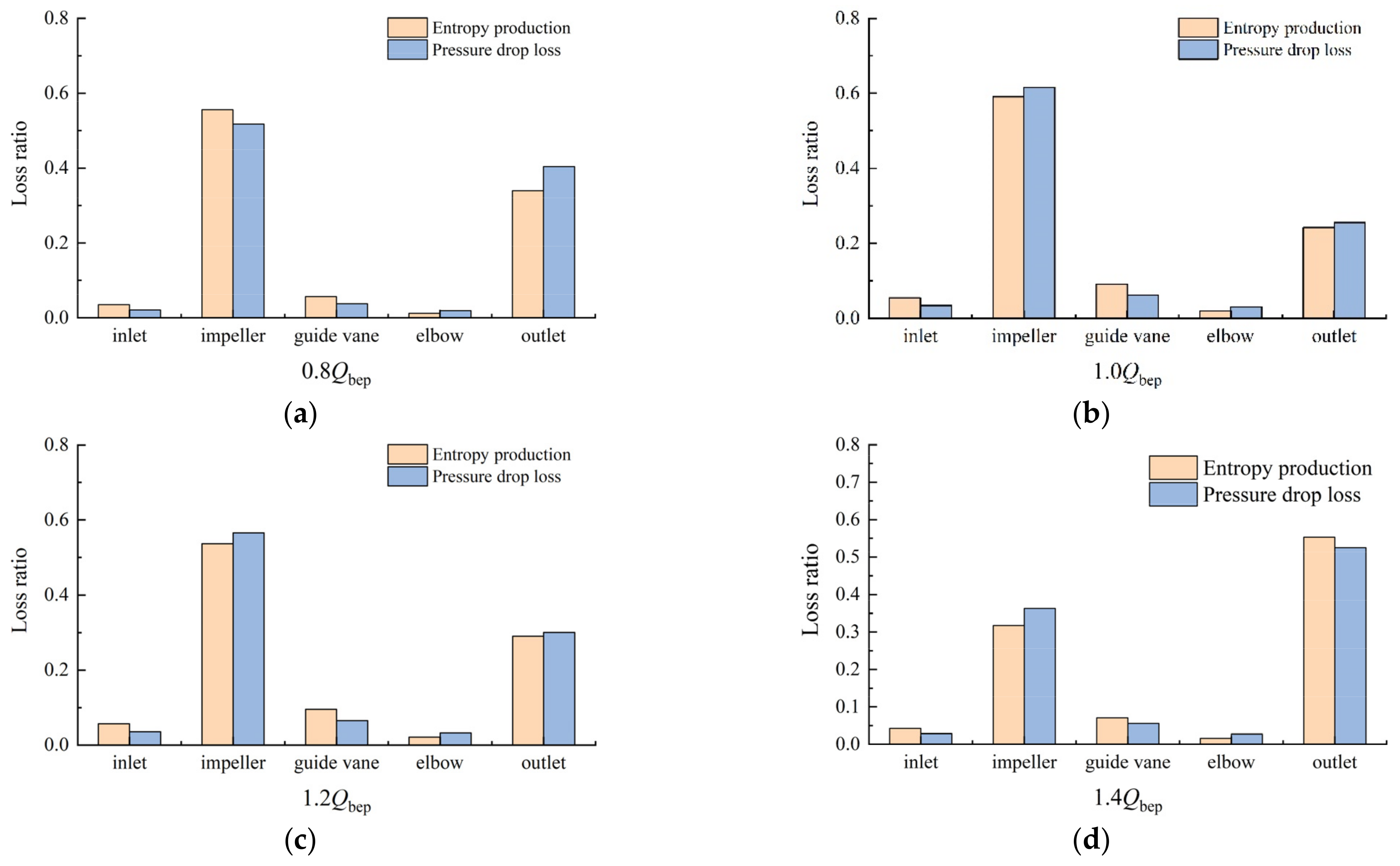
With regard to prove the effectiveness of using entropy production theory to evaluate the hydraulic loss in the axial-flow PAT, it is necessary to compare the hydraulic loss calculated by the pressure drop and entropy production. Figure 6 reflects the loss ratio of head drop loss and entropy production of different flow components in axial-flow PAT at various flow rates, and the loss is normalized into the ratio of flow component loss to the total conduit loss. At different flow rates, it is clear that the entropy production and pressure drop loss of each component have a similar trend, indicating that entropy production could be applied to evaluate the head loss of the axial-flow PAT to a degree. It is known that the loss of the impeller and the dustpan-shape conduit are the main components of hydraulic loss, which occupies a considerable proportion of the entire passage.
4.3. Entropy Production of Each Component of Axial-Flow PAT
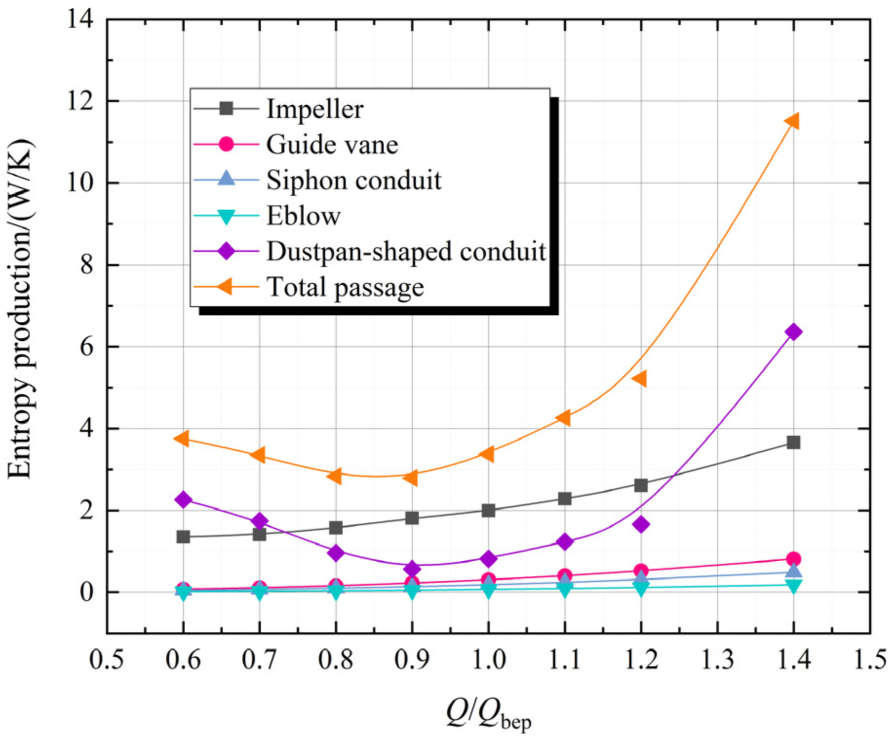
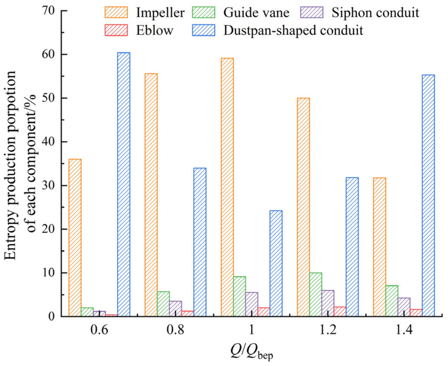
Figure 7 reflects the variation law of entropy production with flow rate of each component of the axial-flow PAT. As the flow rate goes up, the total entropy production of entire passage first decreases slightly and then increases significantly. At 0.9 Q/Qbep, the entropy production value of the entire passage is the smallest with the entropy production of 2.79 W/K. However, the entropy production of entire passage is the largest at 1.4 Q/Qbep, reaching 11.51 W/K. The entropy production of impeller, siphon conduit, elbow and guide vane all increase steadily as the flow rate goes up, and the entropy production of impeller domain increases the most. However, the entropy production value of dustpan-shaped conduit showed a trend of decreasing first and then increasing rapidly, indicating that the entropy production of dustpan-shaped conduit is extremely sensitive to change in flow rate. It can be seen from Figure 8 that the proportion of the entropy production in the impeller domain to the entire passage increases as the flow rate expands. At 1.0Qbep, the entropy production proportion of the impeller domain is the largest, reaching 59.11%. However, the entropy production proportion in the dustpan-shaped conduit shows the opposite trend. The entropy production proportions of siphon conduit, elbow and guide vane are maintained at a relatively low level. The proportion of entropy production also increases slightly along with the increasing of flow rate.
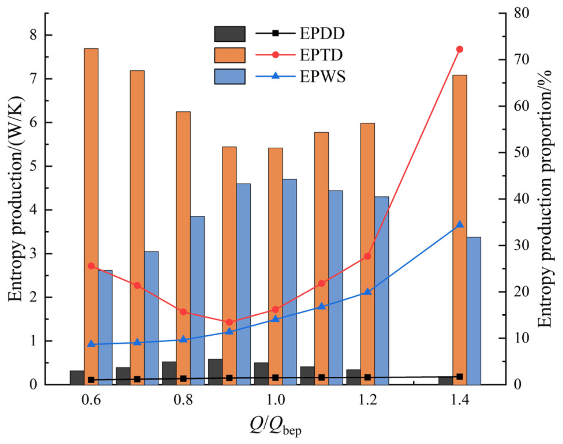
Among the discussion of entropy production theory, we can know that the total entropy production consists of local entropy production and entropy production by wall shear (EPWS), and the local entropy production includes the entropy production by direct dissipation (EPDD) and entropy production by turbulent dissipative (EPTD). The EPTD increases due to the presence of vortices, backflow and other undesirable flow regime throughout the flow passage, while the EPWS is mainly related to the friction loss between the flow and the wall near wall region. Figure 9 reflects the variation law of the three forms of entropy production and their proportion of the total entropy production in the whole passage against various flow rate. The EPDD remains at a low level with no obvious fluctuation along with the variation of flow rate. The EPTD is the smallest near the 1.0Qbep condition, and then increases rapidly to 7.67 W/K at 1.4Qbep condition. The EPWS of the whole passage shows a positive correlation with the flow rate. The EPTD proportion decreases and then increases as the flow rate becomes larger, with the smallest proportion occurring at 1.0Qbep condition with a EPTD proportion of 51.0%. In contrast, the EPWS proportion increases and then decreases with the increase in flow rate, with the maximum value at 1.0Qbep of 44.3%.
4.4. LEPR Distribution of Impeller
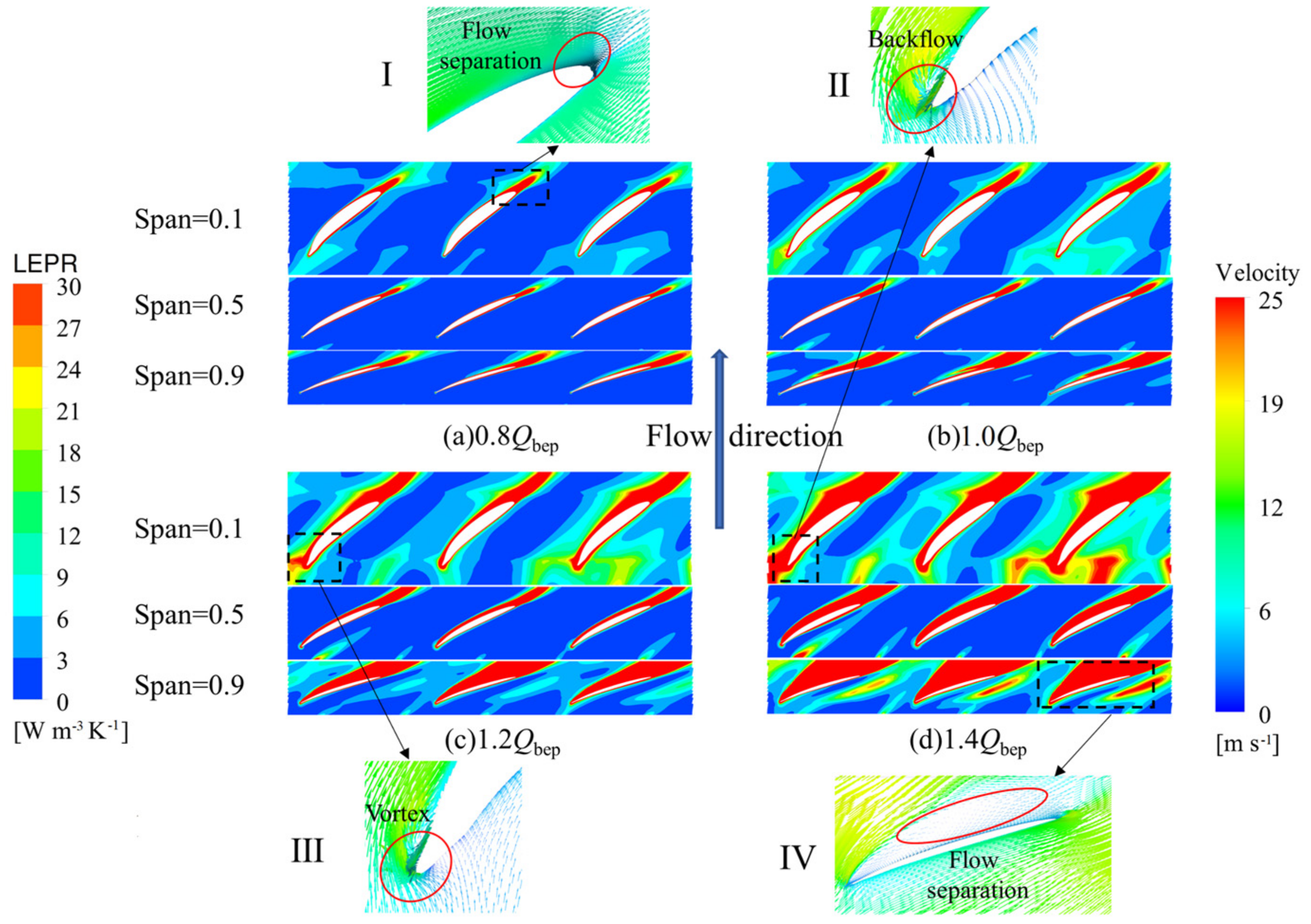
As the core part of the axial-flow PAT, the impeller exists the major energy conversion between the blades and the fluid. Hydraulic loss occurs inevitably in this energy conversion process. It is known from Figure 7 and Figure 8 that entropy production in impeller domain occupies a large proportion in the entire passage. In order to clarify the reason for the high LEPR in the impeller domain, the LEPR distribution and local velocity vector at various spans of the impeller is displayed in Figure 10. Span is the dimensionless distance from the impeller hub to the shroud, defined as ( is the radius of the hub, and is the diameter of the impeller). The high LEPR region is mainly concentrated on the leading edge and trailing edge of the impeller at different spans, and the high LPER region expands as the flow rate goes up. At 0.8Qbep flow rate, a small area of high LEPR appears at the blade trailing edge, which is associated with the flow separation phenomenon at the blade trailing edge (Figure 10I). When the flow enters the impeller axially, there is an angle between the blade and the pump axis, so the flow will have an impact on the leading edge of the blade. As the flow rate continues to increase (1.0Qbep, 1.4Qbep), the flow impact at the blade leading edge becomes more obvious. The flow obviously separated from the blade surface after flowing through the leading edge of the blade, as shown in Figure 10IV. Meanwhile, there was a low-speed area on the blade surface, and there was a flow separation phenomenon. The flow impact on the blade leading edge results in flow separation, forming a high speed region at the leading edge of the blade suction, followed by significant vortex and backflow phenomena (Figure 10II,III). At span 0.9, the high LEPR region locates in the blade suction surface and the wake region, and the flow separation phenomenon on the blade suction surface side intensifies as the flow rate goes up. Due to the flow impact effect of the high speed near the blade leading edge, a large area of low velocity zone is formed on the blade suction surface and it expands from leading edge to the impeller outlet.
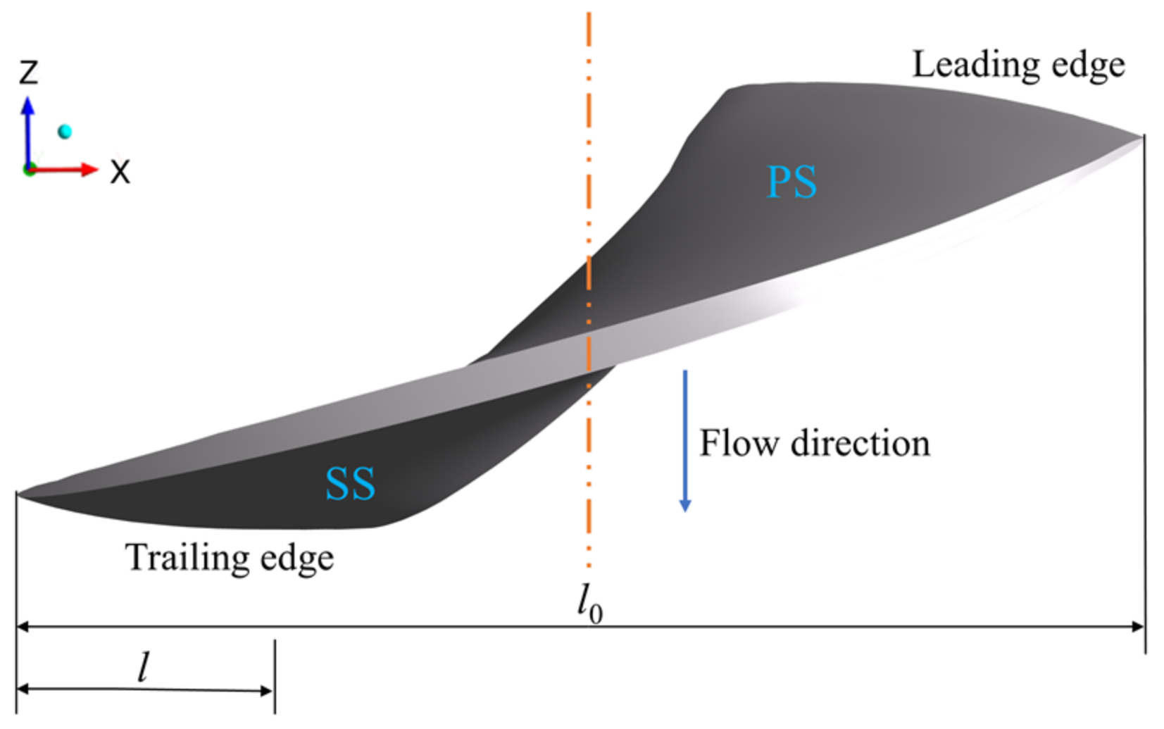
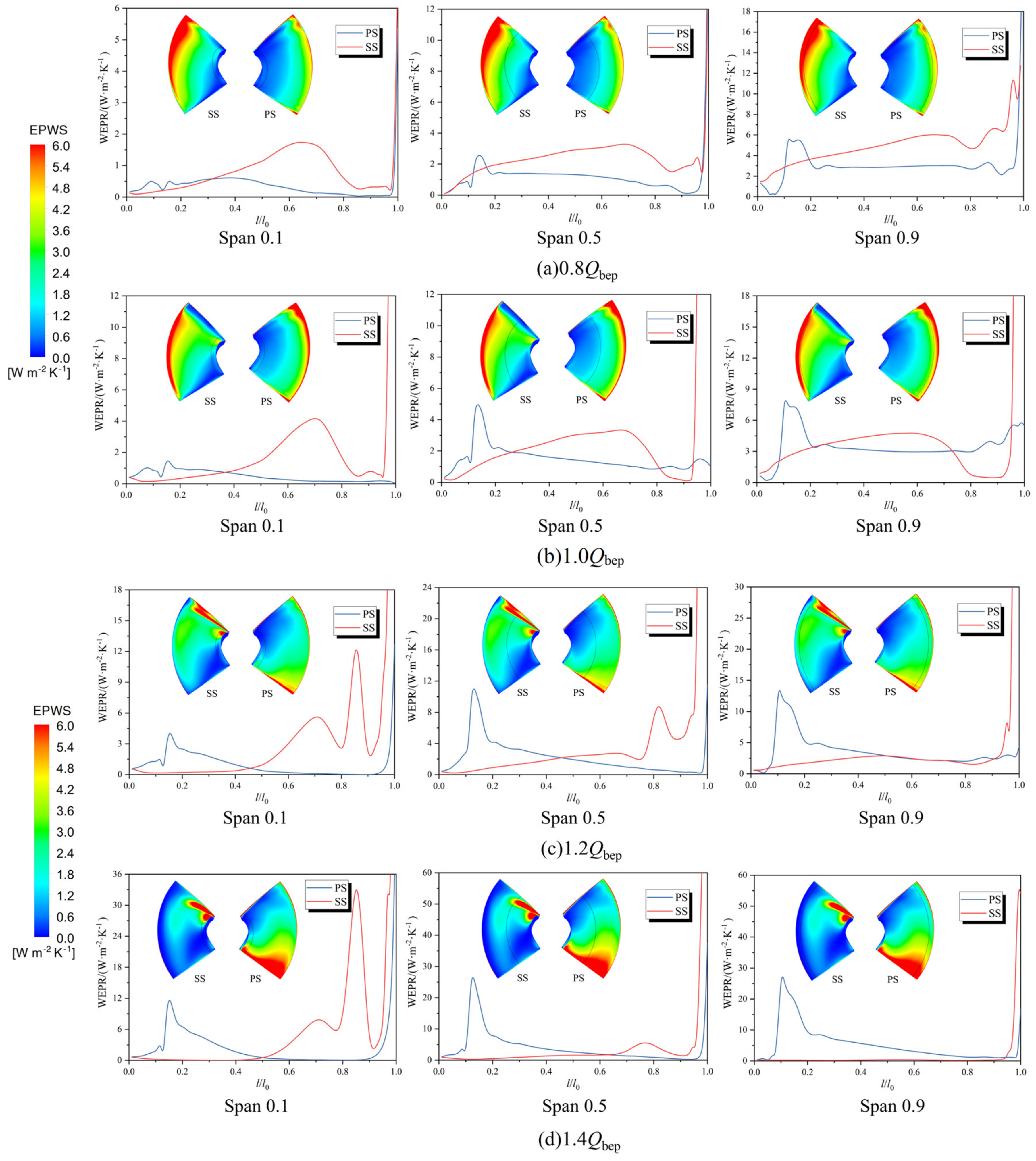
The entropy production by wall shear in the whole passage of the axial-flow PAT occupies a considerable part of the entropy production proportion (Figure 9). The impeller is the most important part of the axial-flow PAT, so it is important to clarify the distribution of entropy production rate induced by wall shear (EPWS) of the impeller to understand the mechanism of energy dissipation in the impeller. Figure 11 reflects the parameters of single blade, l0 is the chord length of the blade, and l/l0 represents the relative chord length position. Figure 12 displays the distribution of EPWS with different spans at four typical flow conditions. At different flow rates, the EPWS of impeller blade is much larger near 0.9 span, indicating that the wall shear stress and velocity are much larger near the impeller shroud. The wall friction loss of fluid and impeller blades is mainly concentrated on the tip clearance. The EPWS of blade pressure surface (PS) increases with the increase in l/l0 at different flow rates and spans, reaching a peak value near l/l0 = 0.12. The EPWS of the blade suction surface (SS) generally shows a trend of gradually increasing as the l/l0 rises. However, there is a steep increase in EPWS on the blade pressure surface near l/l0 = 0.90, which is related to the flow impact on the blade inlet. At low flow condition (0.8Qbep), the high EPWS region locates in the blade leading edge. The EPWS of the blade suction surface is significantly larger than the pressure surface, as the local low pressure near the suction surface can easily cause the unsteady flow regime and the occurrence of backflow phenomenon as well as the greater energy dissipation. At high flow conditions (1.2Qbep, 1.4Qbep), the high EPWS region on the suction surface shrinks significantly and moves to the blade leading edge, in contrast, the high EPWS region on the pressure surface becomes larger and moves to the trailing edge.
4.5. LEPR and Streamline Distribution of Guide Vane
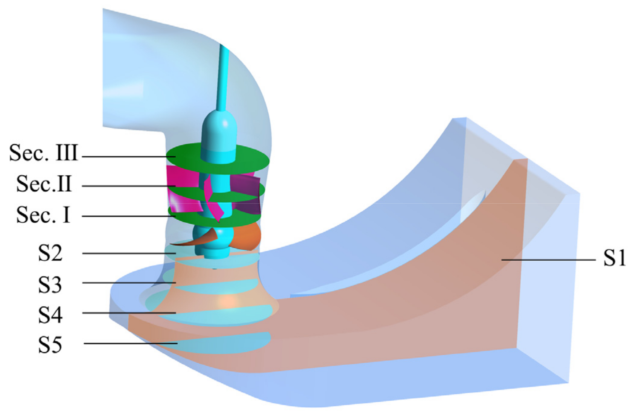
Figure 13 shows the schematic diagram of cross sections in the guide vane and dustpan-shaped conduit. The guide vane plays a role in smoothing the flow pattern of fluid entering the impeller domain when the axial-flow PAT in a turbine mode. Sec. I, Sec. II and Sec. III are located in the inlet, middle and outlet sections of the guide vane, respectively. Section S1 is the symmetric plane of the dustpan-shaped conduit, and the vertical distances between sections S2, S3, S4 and S5 and the impeller center are 0.2 D, 0.5 D, 0.8 D and 1.1 D, respectively (D is the impeller diameter).
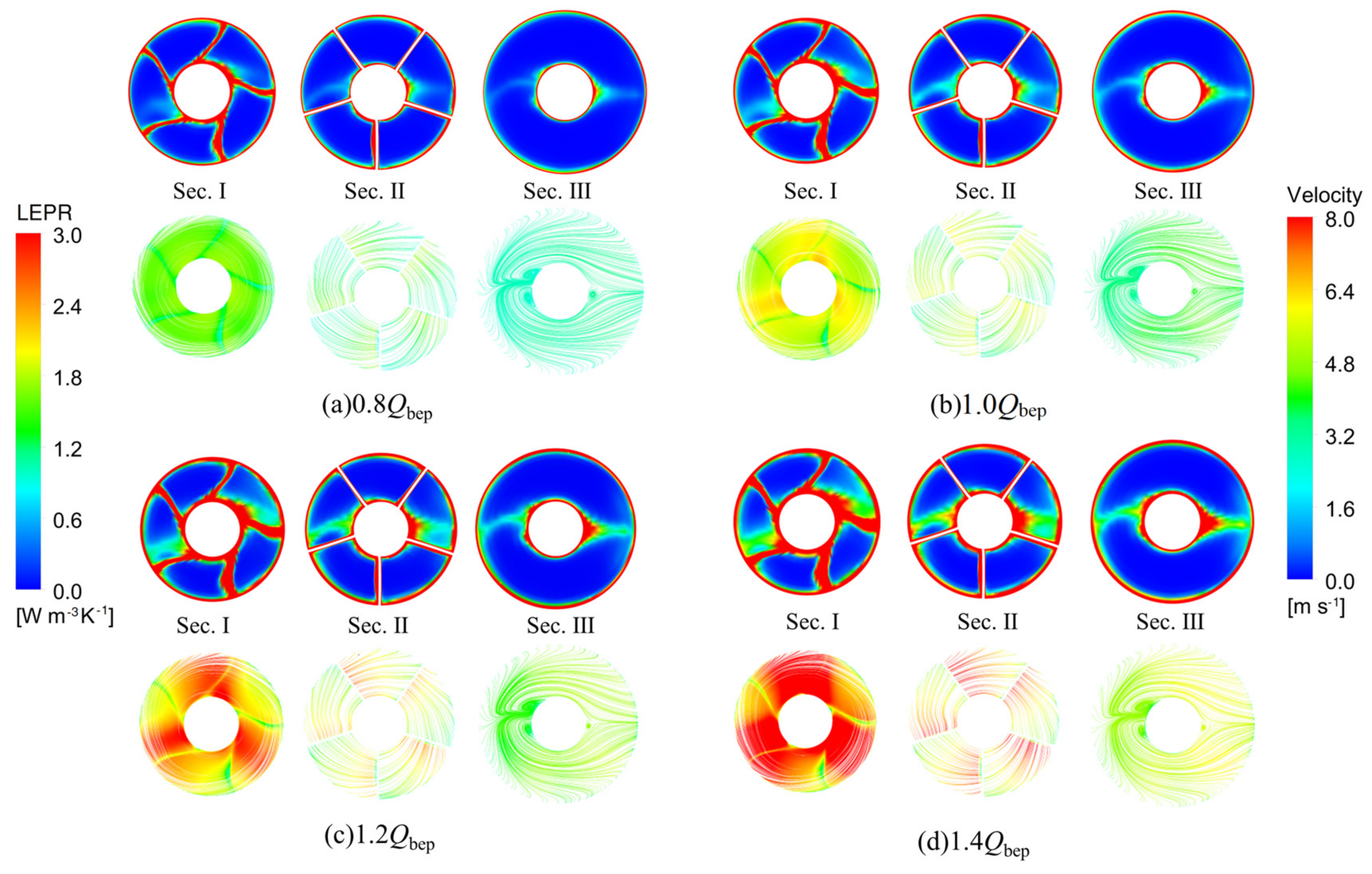
The LEPR and streamline distribution of each section of the guide vane at different flow rates are shown in Figure 14. The guide vane blades divide the guide vane domain into five channels uniformly. The LEPR distribution of section Sec. I and Sec. II is similar, the LEPR in the center of the five channels is low, and there are high LEPR near the blade and shroud. The generation of high LEPR near the blade and wall is related to the significant velocity gradient between the mainstream region and the boundary layer near the wall as well as the guiding effect of the guide vane blades. As the flow rate rises, the increasing flow velocity in the guide vane results in a larger velocity gradient and friction loss near wall region, which in turn causes the expansion of the high LEPR region. The streamline distribution of the three cross-sections and the distribution of LEPR have an obviously similar trend, and the streamline distribution of Sec. I and Sec. II show the same distribution pattern as five equal spacings. The streamline distortion exists in Sec. III cross-section near the hub, which indicates that there is a vortex or flow separation phenomenon, and the streamline distortion location coincides with the high LEPR region of Sec. III cross-section.
4.6. LEPR and Streamline Distribution of Dustpan-Shaped Conduit
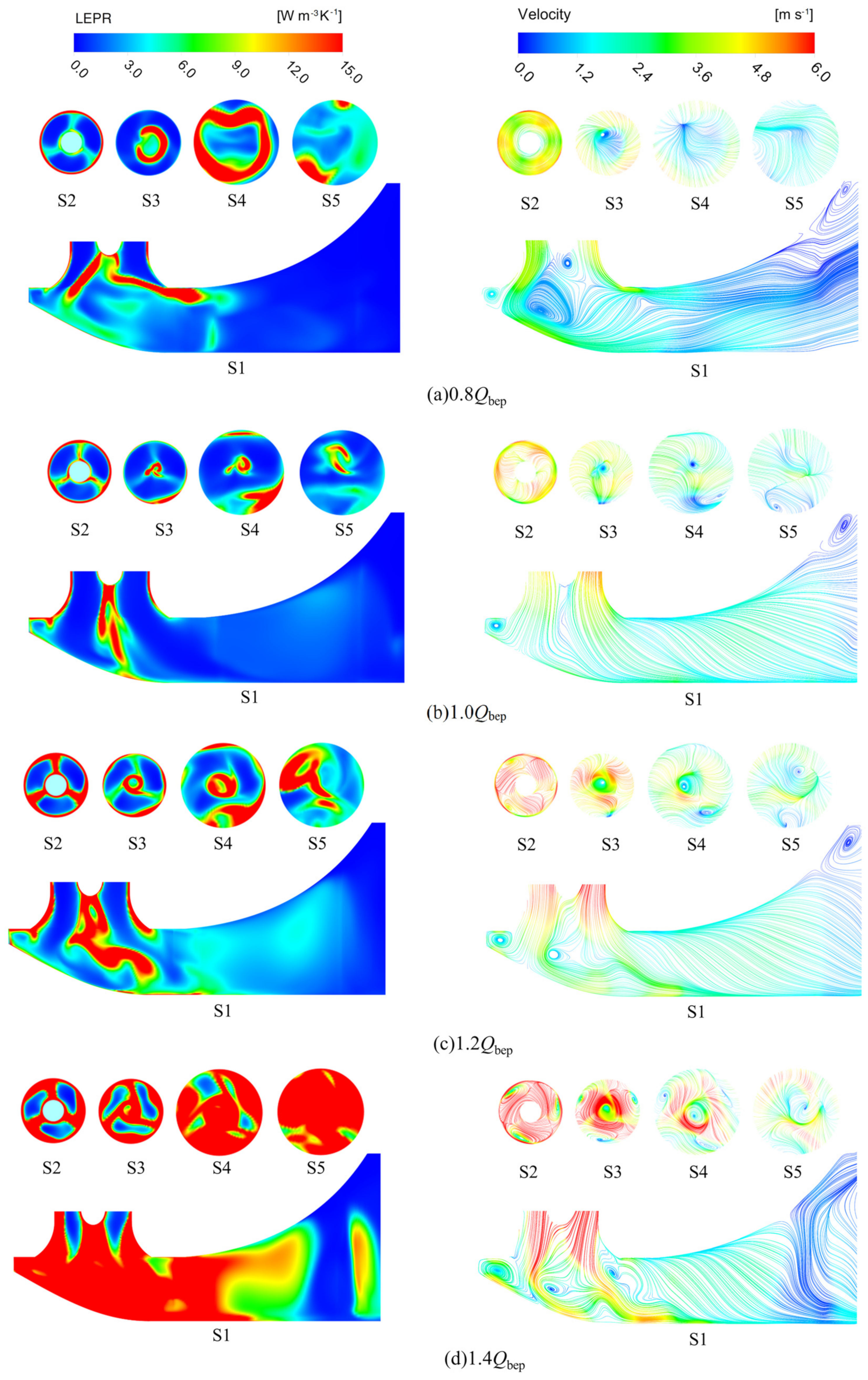
The proportion of entropy production in dustpan-shaped conduit to entropy production of whole passage varies from 24.2% to 60.4% at different flow rates (Figure 8). The entropy production proportion of the dustpan-shaped conduit is very sensitive to the variation of the flow rate, and the proportion is the smallest at 1.0Qbep with the value of 24.2%, while reaching 60.4% at 1.4Qbep. In order to investigate the energy dissipation mechanism in the dustpan-shaped conduit, five typical cross sections were set up in the in dustpan-shaped conduit, as shown in Figure 11. The fluid flows out from the impeller, it still has a large kinetic energy, and the flow velocity gradually decreases and the pressure gradually increases in the dustpan-shaped conduit. The dustpan-shaped conduit plays the role of recovering part of the kinetic energy. Under the condition of 0.8Qbep, the LEPR area of each section is small while the LEPR area increases significantly along with the rising of flow rate. Combining with the streamline diagram of each section, it can be found that the greater the flow rate, the higher of velocity and the more chaotic the flow pattern. In Figure 15, there is a significant high LEPR region near the dustpan-shaped conduit center (sections S2, S3, S4 and S5), and the high LEPR region develops obliquely from the guide cap along with the flow direction to outlet. In addition, the twisted streamline of section S1 near the center of the dustpan-shaped conduit (Figure 15c,d) indicates the presence of an obvious spiral vortex zone, which is associated with the rotation of the impeller and the downward flow trend. It is clear that with the flow rate going up, the flow velocity and vortex intensity at the dustpan-shaped conduit inlet increase significantly, leading to an increase in the turbulence of the flow pattern. Consequently, a surge of LEPR in the dustpan-shaped conduit appears at high flow rates. Chaotic flow patterns and vortices are the essential sources of entropy production and hydraulic losses of the dustpan-shaped conduit.
5. Conclusions
In this paper, the energy dissipation law in flow passage of the axial-flow PAT is analyzed at various flow conditions via entropy production theory. Additionally, the validity of the numerical simulation is verified compared with experimental results. Moreover, the comparison of the hydraulic losses calculated by the pressure drop and entropy production theory shows the effectiveness of entropy production theory to assess the energy loss distribution of the axial-flow PAT.
The entropy production inside the entire passage of the axial-flow PAT is minimum near the optimum flow condition 1.0Qbep. Impeller domain and dustpan-shaped conduit are the essential sources of energy loss in the whole passage of the axial-flow PAT, and the entropy production proportion of impeller and dustpan-shaped conduit accounts for 59.11% and 24.24%, respectively, at the 1.0Qbep. The entropy production proportion of the impeller first increases and then declines as the flow rate goes up, but the entropy production proportion of the dustpan-shaped conduit shows the opposite trend. Moreover, the entropy production in the dustpan-shaped conduit is much more sensitive to the variation of flow rate than other components in the axial-flow PAT.
The proportion of EPDD in the total entropy production of entire passage is less than 5% at different flow rates. The proportion of EPTD is more than half of the total entropy production, and it occupies a dominant position in the entire passage. The EPWS of the entire passage shows a positive correlation with the flow rate. The proportion of EPTD is smallest at 1.0Qbep condition, but the proportion still reaches 51%. In contrast, the proportion of EPWS increases and then decreases along with the flow rate going up, with the maximum value of 44.3% at 1.0Qbep.
The turbulent dissipation of the impeller mainly occurs near the blade leading edge and trailing edge. The energy dissipation in impeller domain at high flow rate is very large, which is mainly associated with the strong flow impact at the leading edge of the blade and the high-speed flow forming a low-pressure region near the blade suction surface. The formation of low-pressure regions further induces undesirable flow regimes such as local vortices and flow separation, thus leading to high energy dissipation. The EPWS of the impeller blade is relatively large near the shroud. After the flow rate goes up, the high EPWS region on the suction side moves to blade leading edge, while the high EPWS region on the pressure side moves to the trailing edge. The high LEPR of the dustpan-shaped conduit is mainly related to the spiral vortex formed by the high-speed flow out of the impeller. The increase in the flow velocity at large flow rate intensifies the chaos of the flow in the dustpan-shaped conduit, leading to the increase in the LEPR.
Axial-flow PATs operating in turbine mode inevitably introduce problems of low efficiency and high flow loss. After determining the specific location of the losses and the main causes of the losses, it is possible to carry out targeted measures to reduce the losses. This paper can offer a reference for future work on the optimization and design of hydraulic structures aiming at the minimum entropy production rate to advance the energy performance of axial-flow PATs. In the follow-up study, research work can be carried out such as optimizing the profile of the blade, the thickness of the blade, and the geometric size control of the dustpan-shaped conduit (the width of the conduit, the profile of the horn tube, and the radius of the dustpan-shaped conduit).
Author Contributions
Conceptualization, F.Y. and Z.L.; methodology, F.Y.; software, Z.L. and D.J.; validation, F.T. and D.J.; formal analysis, Z.L.; investigation, F.Y.; resources, S.S.; data curation, Y.C.; writing—original draft preparation, Z.L.; writing—review and editing, F.T.; visualization, Y.C.; supervision, S.S.; funding acquisition, F.Y. All authors have read and agreed to the published version of the manuscript.
Funding
This research was supported by the National Natural Science Foundation of China (Grant No. 51609210, 51779214), Major Projects of the Natural Science Foundation of the Jiangsu Higher Education Institutions of China (Grant No. 20KJA570001), Open Project of Jiangxi Research Center on Hydraulic Structures (Grant No. 2021SKSG06) and Postgraduate Research & Practice Innovation Program of Jiangsu Province (Grant No. SJCX21_1583).
Institutional Review Board Statement
Not applicable.
Informed Consent Statement
Not applicable.
Data Availability Statement
All data are available in this paper.
Conflicts of Interest
The authors declare no conflict of interest. The funders had no role in the design of the study; in the collection, analyses, or interpretation of data; in the writing of the manuscript; or in the decision to publish the results.
References
- Zhao, X.; Ma, X.; Chen, B.; Shang, Y.; Song, M. Challenges toward carbon neutrality in China: Strategies and countermeasures. Resour. Conserv. Recycl. 2022, 176, 105959. [Google Scholar] [CrossRef]
- Qiu, T.; Wang, L.; Lu, Y.; Zhang, M.; Qin, W.; Wang, S.; Wang, L. Potential assessment of photovoltaic power generation in China. Renew. Sustain. Energy Rev. 2022, 154, 111900. [Google Scholar] [CrossRef]
- Shen, J.-J.; Cheng, C.-T.; Jia, Z.-B.; Zhang, Y.; Lv, Q.; Cai, H.-X.; Wang, B.-C.; Xie, M.-F. Impacts, challenges and suggestions of the electricity market for hydro-dominated power systems in China. Renew. Energy 2022, 187, 743–759. [Google Scholar] [CrossRef]
- Kaunda, C.S.; Kimambo, C.Z.; Nielsen, T.K. A technical discussion on microhydropower technology and its turbines. Renew. Sustain. Energy Rev. 2014, 35, 445–459. [Google Scholar] [CrossRef]
- Binama, M.; Su, W.-T.; Li, X.-B.; Li, F.-C.; Wei, X.-Z.; An, S. Investigation on pump as turbine (PAT) technical aspects for micro hydropower schemes: A state-of-the-art review. Renew. Sustain. Energy Rev. 2017, 79, 148–179. [Google Scholar] [CrossRef]
- Barrio, R.M.; Fernández, J.; Blanco, E.F.; Parrondo, J.L.; Marcos, A. Performance characteristics and internal flow patterns in a reverse-running pump–turbine. Proc. Inst. Mech. Eng. Part C J. Mech. Eng. Sci. 2012, 226, 695–708. [Google Scholar] [CrossRef]
- Yang, F.; Li, Z.; Yuan, Y.; Lin, Z.; Zhou, G.; Ji, Q. Study on vortex flow and pressure fluctuation in dustpan-shaped conduit of a low head axial-flow pump as turbine. Renew. Energy 2022, 196, 856–869. [Google Scholar] [CrossRef]
- Štefan, D.; Rossi, M.; Hudec, M.; Rudolf, P.; Nigro, A.; Renzi, M. Study of the internal flow field in a pump-as-turbine (PaT): Numerical investigation, overall performance prediction model and velocity vector analysis. Renew. Energy 2020, 156, 158–172. [Google Scholar] [CrossRef]
- Liu, J.; Liu, S.; Wu, Y.; Jiao, L.; Wang, L.; Sun, Y. Numerical investigation of the hump characteristic of a pump–turbine based on an improved cavitation model. Comput. Fluids 2012, 68, 105–111. [Google Scholar] [CrossRef]
- Ran, H.; Luo, X.; Zhu, L.; Zhang, Y.; Wang, X.; Xu, H. Experimental study of the pressure fluctuations in a pump turbine at large partial flow conditions. Chin. J. Mech. Eng. 2012, 25, 1205–1209. [Google Scholar] [CrossRef]
- Li, Z.; Bi, H.; Karney, B.; Wang, Z.; Yao, Z. Three-dimensional transient simulation of a prototype pump-turbine during normal turbine shutdown. J. Hydraul. Res. 2017, 55, 520–537. [Google Scholar] [CrossRef]
- Kim, S.-J.; Suh, J.-W.; Yang, H.-M.; Park, J.; Kim, J.-H. Internal flow phenomena of a Pump–Turbine model in turbine mode with different Thoma numbers. Renew. Energy 2022, 184, 510–525. [Google Scholar] [CrossRef]
- Olimstad, G.; Nielsen, T.; Børresen, B. Dependency on Runner Geometry for Reversible-Pump Turbine Characteristics in Turbine Mode of Operation. J. Fluids Eng. 2012, 134, 121102. [Google Scholar] [CrossRef]
- Liu, Y.; Tan, L. Tip clearance on pressure fluctuation intensity and vortex characteristic of a mixed flow pump as turbine at pump mode. Renew. Energy 2018, 129, 606–615. [Google Scholar] [CrossRef]
- Yang, S.-S.; Kong, F.-Y.; Chen, H.; Su, X.-H. Effects of Blade Wrap Angle Influencing a Pump as Turbine. J. Fluids Eng. 2012, 134, 061102. [Google Scholar] [CrossRef]
- Li, D.; Gong, R.; Wang, H.; Xiang, G.; Wei, X.; Qin, D. Entropy production analysis for hump characteristics of a pump turbine model. Chin. J. Mech. Eng. 2016, 29, 803–812. [Google Scholar] [CrossRef]
- Hou, H.; Zhang, Y.; Li, Z. A numerically research on energy loss evaluation in a centrifugal pump system based on local entropy production method. Therm. Sci. 2017, 21, 1287–1299. [Google Scholar] [CrossRef]
- Zhou, L.; Hang, J.; Bai, L.; Krzemianowski, Z.; El-Emam, M.A.; Yasser, E.; Agarwal, R. Application of entropy production theory for energy losses and other investigation in pumps and turbines: A review. Appl. Energy 2022, 318, 119211. [Google Scholar] [CrossRef]
- Kock, F.; Herwig, H. Entropy production calculation for turbulent shear flows and their implementation in CFD codes. Int. J. Heat Fluid Flow 2005, 26, 672–680. [Google Scholar] [CrossRef]
- Herwig, H.; Kock, F. Direct and indirect methods of calculating entropy generation rates in turbulent convective heat transfer problems. Heat Mass Transf. 2007, 43, 207–215. [Google Scholar] [CrossRef]
- Kock, F.; Herwig, H. Local entropy production in turbulent shear flows: A high-Reynolds number model with wall functions. Int. J. Heat Mass Transf. 2004, 47, 2205–2215. [Google Scholar] [CrossRef]
- Duan, L.; Wu, X.; Ji, Z.; Xiong, Z.; Zhuang, J. The flow pattern and entropy generation in an axial inlet cyclone with reflux cone and gaps in the vortex finder. Powder Technol. 2016, 303, 192–202. [Google Scholar] [CrossRef]
- Duan, L.; Wu, X.; Ji, Z.; Fang, Q. Entropy generation analysis on cyclone separators with different exit pipe diameters and inlet dimensions. Chem. Eng. Sci. 2015, 138, 622–633. [Google Scholar] [CrossRef]
- Gong, R.; Wang, H.; Chen, L.; Li, D.; Zhang, H.; Wei, X. Application of entropy production theory to hydro-turbine hydraulic analysis. Sci. China Technol. Sci. 2013, 56, 1636–1643. [Google Scholar] [CrossRef]
- Silva-Llanca, L.; del Valle, M.; Ortega, A.; Díaz, A.J. Cooling effectiveness of a data center room under overhead airflow via entropy generation assessment in transient scenarios. Entropy 2019, 21, 98. [Google Scholar] [CrossRef]
- Ries, F.; Li, Y.; Klingenberg, D.; Nishad, K.; Janicka, J.; Sadiki, A. Near-wall thermal processes in an inclined impinging jet: Analysis of heat transport and entropy generation mechanisms. Energies 2018, 11, 1354. [Google Scholar] [CrossRef]
- Hou, H.; Zhang, Y.; Zhou, X.; Zuo, Z.; Chen, H. Optimal hydraulic design of an ultra-low specific speed centrifugal pump based on the local entropy production theory. Proc. Inst. Mech. Eng. Part A J. Power Energy 2019, 233, 715–726. [Google Scholar] [CrossRef]
- Ji, L.; Li, W.; Shi, W.; Chang, H.; Yang, Z. Energy characteristics of mixed-flow pump under different tip clearances based on entropy production analysis. Energy 2020, 199, 117447. [Google Scholar] [CrossRef]
- Pan, S.S.; Peng, X.X. Physical Mechanism of Cavitation; National Defense Industry Press: Beijing, China, 2013. [Google Scholar]
- Yang, F.; Li, Z.; Hu, W.; Liu, C.; Jiang, D.; Liu, D.; Nasr, A. Analysis of flow loss characteristics of slanted axial-flow pump device based on entropy production theory. R. Soc. Open Sci. 2022, 9, 211208. [Google Scholar] [CrossRef]
- Escaler, X.; Egusquiza, E.; Farhat, M.; Avellan, F.; Coussirat, M. Detection of cavitation in hydraulic turbines. Mech. Syst. Signal Process 2006, 20, 983–1007. [Google Scholar] [CrossRef] [Green Version]
- Wang, C.; Zhang, Y.; Yuan, Z.; Ji, K. Development and application of the entropy production diagnostic model to the cavitation flow of a pump-turbine in pump mode. Renew. Energy 2020, 154, 774–785. [Google Scholar] [CrossRef]
- Lai, F.; Huang, M.; Wu, X.; Nie, C.; Li, G. Local entropy generation analysis for cavitation flow within a centrifugal pump. J. Fluids Eng. 2022, 144, 101206. [Google Scholar] [CrossRef]
- Fei, Z.; Zhang, R.; Xu, H.; Feng, J.; Mu, T.; Chen, Y. Energy performance and flow characteristics of a slanted axial-flow pump under cavitation conditions. Phys. Fluids 2022, 34, 035121. [Google Scholar] [CrossRef]
- Lu, G.; Zuo, Z.; Sun, Y.; Liu, D.; Tsujimoto, Y.; Liu, S. Experimental evidence of cavitation influences on the positive slope on the pump performance curve of a low specific speed model pump-turbine. Renew. Energy 2017, 113, 1539–1550. [Google Scholar] [CrossRef]
- Widmer, C.; Staubli, T.; Ledergerber, N. Unstable Characteristics and Rotating Stall in Turbine Brake Operation of Pump-Turbines. J. Fluids Eng. 2011, 133, 041101. [Google Scholar] [CrossRef]
- Herwig, H.; Kock, F. Local entropy production in turbulent shear flows: A tool for evaluating heat transfer performance. J. Therm. Sci. 2006, 15, 159–167. [Google Scholar] [CrossRef]
- Mathieu, J.; Scott, J. An Introduction to Turbulent Flow; Cambridge University Press: Cambridge, UK, 2000. [Google Scholar]
- Li, D.; Wang, H.; Qin, Y.; Han, L.; Wei, X.; Qin, D. Entropy production analysis of hysteresis characteristic of a pump-turbine model. Energy Convers. Manag. 2017, 149, 175–191. [Google Scholar] [CrossRef]
- Yang, F.; Li, Z.; Fu, J.; Lv, Y.; Ji, Q.; Jian, H. Numerical and experimental analysis of transient flow field and pressure pulsations of an axial-flow pump considering the pump–pipeline interaction. J. Mar. Sci. Eng. 2022, 10, 258. [Google Scholar] [CrossRef]
- Menter, F.R. Two-equation eddy-viscosity turbulence models for engineering applications. AIAA J. 1994, 32, 1598–1605. [Google Scholar] [CrossRef]
- Wilcox, D. Multiscale model for turbulent flows. AIAA J. 1988, 26, 1311–1320. [Google Scholar] [CrossRef]
- Spalart, P.; Shur, M. On the sensitization of turbulence models to rotation and curvature. Aerosp. Sci. Technol. 1997, 1, 297–302. [Google Scholar] [CrossRef]
- Guo, Q.; Zhou, L.; Wang, Z.; Liu, M.; Cheng, H. Numerical simulation for the tip leakage vortex cavitation. Ocean Eng. 2018, 151, 71–81. [Google Scholar] [CrossRef]
- Musa, O.; Changsheng, Z.; Xiong, C.; Lunkun, G. Prediction of swirling cold flow in a solid-fuel ramjet engine with a modified rotation/curvature correction SST turbulence model. Appl. Therm. Eng. 2016, 105, 737–754. [Google Scholar] [CrossRef]
- Ali, S.; Elliott, K.J.; Savory, E.; Zhang, C.; Martinuzzi, R.J.; Lin, W.E. Investigation of the Performance of Turbulence Models With Respect to High Flow Curvature in Centrifugal Compressors. J. Fluids Eng. 2016, 138, 051101. [Google Scholar] [CrossRef]
- Roache, P.J. Quantification of uncertainty in computational fluid dynamics. Annu. Rev. Fluid Mech. 1997, 29, 123–160. [Google Scholar] [CrossRef]
- Celik, I.B.; Ghia, U.; Roache, P.J.; Freitas, C.J.; Coleman, H.; Raad, P.E. Procedure for estimation and reporting of uncertainty due to discretization in CFD applications. J. Fluids Eng. 2008, 130, 078001. [Google Scholar] [CrossRef] [Green Version]
Figure 1.
Geometric structure of the axial-flow PAT.

Figure 2.
Test bench and physical model of the vertical axial-flow PAT.

Figure 3.
The grid of the axial-flow PAT computational domain.

Figure 4.
Grid number independence of the axial-flow PAT.

Figure 5.
Performance curve of the axial-flow PAT: (a) head and (b) efficiency.

Figure 6.
Comparison of pressure drop loss and entropy production of each component at different flow rates: (a) 0.8Qbep, (b) 1.0Qbep, (c) 1.2Qbep, and (d) 1.4Qbep.
Figure 6.
Comparison of pressure drop loss and entropy production of each component at different flow rates: (a) 0.8Qbep, (b) 1.0Qbep, (c) 1.2Qbep, and (d) 1.4Qbep.

Figure 7.
Variation of entropy production each component at various flow rates.

Figure 8.
Entropy production proportion of each component.

Figure 9.
Variation of 3 forms of entropy production in the whole passage.

Figure 10.
Distribution of LEPR at various impeller spans and local velocity vector diagrams: (I) Blade trailing edge at 0.8Qbep; (II) Blade leading edge at 1.4Qbep; (III) Blade leading edge at 1.2Qbep; (IV) Blade region at 1.4Qbep.
Figure 10.
Distribution of LEPR at various impeller spans and local velocity vector diagrams: (I) Blade trailing edge at 0.8Qbep; (II) Blade leading edge at 1.4Qbep; (III) Blade leading edge at 1.2Qbep; (IV) Blade region at 1.4Qbep.

Figure 11.
The parameters of a single impeller blade.

Figure 12.
The EPWS distribution on impeller blade surfaces at various flow rates.

Figure 13.
The cross-sections in guide vane and dustpan-shaped conduit.

Figure 14.
LEPR and streamline distribution of the cross sections in guide vane.

Figure 15.
LEPR and streamline distribution in the dustpan-shaped conduit.


Table 1.
Grid discrete error estimation results.
| Parameter | Φ = Efficiency |
|---|---|
| N1, N2, N3 | 6,143,640, 2,746,492, 721,326 |
| r21, r32 | 1.31, 1.56 |
| φ1, φ2, φ3 | 43.64%, 42.82%, 42.13% |
| p | 4.2 |
| , | 44.03%, 42.9% |
| 1.9% | |
| 0.89% | |
| GCI21 | 1.13% |
Publisher’s Note: MDPI stays neutral with regard to jurisdictional claims in published maps and institutional affiliations. |
© 2022 by the authors. Licensee MDPI, Basel, Switzerland. This article is an open access article distributed under the terms and conditions of the Creative Commons Attribution (CC BY) license (https://creativecommons.org/licenses/by/4.0/).
Share and Cite
MDPI and ACS Style
Yang, F.; Li, Z.; Cai, Y.; Jiang, D.; Tang, F.; Sun, S. Numerical Study for Flow Loss Characteristic of an Axial-Flow Pump as Turbine via Entropy Production Analysis. Processes 2022, 10, 1695. https://doi.org/10.3390/pr10091695
AMA Style
Yang F, Li Z, Cai Y, Jiang D, Tang F, Sun S. Numerical Study for Flow Loss Characteristic of an Axial-Flow Pump as Turbine via Entropy Production Analysis. Processes. 2022; 10(9):1695. https://doi.org/10.3390/pr10091695
Chicago/Turabian StyleYang, Fan, Zhongbin Li, Yiping Cai, Dongjin Jiang, Fangping Tang, and Shengjie Sun. 2022. "Numerical Study for Flow Loss Characteristic of an Axial-Flow Pump as Turbine via Entropy Production Analysis" Processes 10, no. 9: 1695. https://doi.org/10.3390/pr10091695
Note that from the first issue of 2016, this journal uses article numbers instead of page numbers. See further details here.