Diffusion Coefficients in Systems Related to Reservoir Fluids: Available Data and Evaluation of Correlations

Abstract

Molecular diffusion determines the time to reach local equilibrium in a reservoir. It can be a main production mechanism in scenarios such as production from fractured reservoirs or tight formation. However, there is a lack of high-pressure diffusion coefficients for reservoir fluids and its related systems. Many correlations exist, but there is no consensus on their accuracy for these systems. We provide a systematic review of the available data for systems related to reservoir fluids, as well as a comprehensive comparison of five commonly used correlations for hydrocarbon mixtures, including the extended Sigmund, Riazi-Whitson, Leahy-Dios-Firoozabadi, Wilke–Chang, and the Hayduk–Minhas correlations. We collected extensive data of diffusion coefficients in binary mixtures related to petroleum fluids and established a database of over 80 binaries and 1600 data points. We also collected the data for gas diffusion in different oils and reservoir fluids, but the data in high-pressure live oils are extremely scarce. The five correlations were evaluated using the binary database, and a few selected correlations using the oil database. None of the correlations show consistent and dominant superiority for all the binary mixtures, although some are better for particular groups/regions. For oils and reservoir fluids, the composition information is often incomplete. Only a few sets allow a comparison between different correlations. Although some trends can be identified from the correlation evaluation, no conclusive recommendation is made for a particular model, due to the data scarcity. The findings underscore the need for more accurate measurement and modeling of gas diffusion in mixtures that are more representative of reservoir fluids at high pressures.

1. Introduction

Molecular diffusion is a relatively slow mass transport phenomenon, in contrast to convection, but it plays a critical role in a system transiting from a non-equilibrium state towards an equilibrium one. Intuitively, it refers to “the net transport of material within a single phase in the absence of mixing” [1]. Unlike convection, i.e., the movement of the bulk phase that is directly driven by the pressure gradient, diffusion is the movement of the components in a phase driven by the chemical potential gradient, which is related to the non-uniform distribution of pressure, temperature, and concentration in space. In this study, our discussion of diffusion is limited to concentration-driven diffusion. Molecular diffusion is the statistical results of the molecular thermal motion. Different from the high-velocity thermal motion of molecules, the velocity of diffusion is much smaller, often becoming a limiting factor for the overall rate of a mass transport process [2].

1.1. Importance for Petroleum Production

Molecular diffusion is important in various areas, including geologic processes (hydrothermal rock alteration, mass transport associated with diagenetic fluxes, and the transport of radiogenic species from nuclear repositories) [3], chemical separation processes (distillation, absorption, and extraction), and biomedical applications (diffusion of nutrients and oxygen through the biocapsule) [4]. In petroleum reservoirs, diffusion can be a critical mass transfer mechanism that directly influences production [5,6].

The solution gas drive is a major recovery mechanism in many petroleum reservoirs [7], especially in their early production stage. As the pressure declines below the bubble-point pressure, the formation and expansion of gas bubbles from the supersaturated oil is a major driving force for oil production. Li and Yortsos [8] showed that the gas bubble growth is directly controlled by diffusion through their modeling of a solution gas drive experiment. For late-stage reservoirs, the trapped oil can be recovered by gas injection. Campbell and Orr [9] performed a series of CO₂ flooding experiments in two-dimensional pore networks etched in glass plates. They observed that much of the residual oil was recovered slowly by diffusion. Similarly, Grogan and Pinczewski [10] developed an idealized one-dimensional pore-scale model to simulate CO₂ diffusion through a water barrier to a trapped oil phase, as well as the subsequent swelling of the oil phase. The model demonstrated that molecular diffusion played a dominant role in the recovery of waterflood residual oil on the micro or pore scale.

Molecular diffusion is particularly important for naturally fractured reservoirs because the dispersive flux through fractures rapidly increases the contact area for diffusion [11,12]. It may even override viscous forces when hydrocarbon or inert gases are injected into fractures with small spacing. Trivedi and Babadagli [13] studied the diffusion process during the flow of solvent (heptane) into the fracture adjacent to the oil saturated matrix by a series of core flooding experiments, and they concluded that the diffusion coefficient was the major controlling parameter, provided that the oil inside the matrix pores was larger in amount than that in the fracture. Alavian and Whitson [14] modeled the CO₂ flooding experiment in chalk performed by Darvish et al. [15]. They reported that vaporization, condensation, and molecular diffusion were the dominant production mechanism in the early stage of the experiment. Hoteit and Firoozabadi [16] presented a field-scale gas injection simulation of diffusion in a fractured reservoir and demonstrated that, at pressures below MMP, molecular diffusion could result in significant recovery enhancement. Alavian and Whitson [17] made both reservoir- and lab-scale simulations for CO₂ injection in the matrix-fracture systems. For all the studied cases, molecular diffusion showed a significant acceleration effect on oil recovery. The impact is related to accelerated CO₂ entry into the matrix block, subsequent effect on gravity-capillary drainage, and capillary-induced displacement, as well as an efficient oil-vaporization/gas-diffusion recovery mechanism. Yanze and Clemens [18] simulated CO₂ injection into a pervasively fractured reservoir. They found that, with a larger viscosity reduction, higher porosities, smaller fracture spacing, lower matrix permeability, and larger block heights (longer drainage times and, hence, more time for diffusion), diffusion became more significant in the increase of the oil recovery. In some cases, the difference in the oil recovery was larger than 25% if diffusion was not included.

The development of unconventional shale or other tight formation relies on horizontal drilling and multi-stage hydraulic fracturing, where diffusion can become critical, due to the large contact area and fracture-matrix interaction. As the need for EOR in unconventional reservoirs increases [19], gas injection, particularly huff-n-puff, becomes more commonly used. Here, diffusion is likely to play a pivotal role in the mass transfer within the matrix, since the convective flow is restricted by the extremely small pores. CH₄ and CO₂ are the two most common injection gas components, and their diffusion in oil has been the focus of some recent experimental and simulation studies. According to a hypothesized recovery mechanism for CO₂ EOR in tight hydraulically fractured systems [20], after the early-stage flooding of the oil in the fractures, oil production from the matrix relied on the swelling of CO₂-permeated oil and vaporization of the light components from oil, both directly related to diffusion. Yu et al. [21] investigated the role of diffusion in CO₂ huff-n-puff by a field-scale simulation, based on typical properties of the Bakken formation, and showed that the diffusion mechanism is more pronounced than the convection one. Wan and Sheng [22] simulated a field-scale natural gas injection into shale using a dual-permeability model and showed that the diffusion contributed 4–8% recovery increase at one pore-volume gas injection. Jin et al. [23] carried out 24-h CH₄ and CO₂ extraction experiments from the tight Bakken cores and argued the importance of diffusion in the penetration of gas into the tight matrix. Alharthy et al. [24] performed CO₂ huff-n-puff experiments with the Bakken cores and simulated both the laboratory and field-scale huff-n-puff. They concluded that the molecular diffusion was one of the major mechanisms, and it contributed to 10–20% oil recovery increase.

Finally, it is worthwhile to mention the importance of diffusion in the production of highly viscous heavy oil and bitumen. Thermal and solvent-based methods are commonly applied in their production. The solvent-based methods, such as vapor extraction (Vapex) [25], consist of reducing the heavy oil/bitumen viscosity by a light solvent. The solvent dissolution rate is significantly affected by molecular diffusion [26]. Butler and Jiang [27] performed a series of Vapex experiments with different solvents and showed that the higher diffusivity provided a higher recovery.

1.2. Diffusion Theories and Correlations

To describe diffusion quantitatively, we need to link the diffusion flux with the diffusion potential. The proportionality factor between the two is called the diffusion coefficient, generally denoted by D. There are many ways to define the diffusion flux and potential, which result in various diffusion coefficients and frameworks in practical use. The diffusion flux can be defined using mole-, mass-, volume-, and solvent-based average reference velocity [28,29]. They provide different diffusion coefficients that can be converted between each other. Mole-based diffusion coefficients are considered in this study. There are two major diffusion frameworks commonly used: Fickian [30] and Maxwell–Stefan (MS) [31]. Both theories were originally developed for binary mixtures and can be extended to multicomponent mixtures [32,33]. Fick’s law in the Fickian framework is the most well-known expression for the diffusion flux. It uses the concentration gradient as the driving force. The MS framework is more rigorous, in the sense that the chemical potential gradient is used as the driving force. Fick’s law can be extended to multicomponent mixtures through the generalized Fickian law. The coefficients in this generalized form can be related to those in the MS equation. For a N_c-component mixture, there are (N_c−1)² independent diffusion coefficients using the generalized Fick’s law, but N_c(N_c−1)/2 MS diffusion coefficients. Obviously, except for a binary mixture, there are more Fickian diffusion coefficients than the MS diffusion coefficients. Despite the different numbers of diffusion coefficients under two frameworks, the MS diffusion coefficients can be converted to the Fickian ones by use of the composition derivatives of chemical potentials. It should be noted that, even for a binary mixture with only one MS or Fickian diffusion coefficient, the conversion is generally needed. However, at the infinite dilution limit, the MS and Fickian diffusion coefficients are the same, since the thermodynamic correction factors used for converting the MS coefficients to the Fickian ones become unity at this limit [2].

For rigorous theoretical analysis and calculation, it is convenient to use the MS framework and diffusion coefficients. Nevertheless, Fick’s law is so widely accepted in common scientific research and engineering practice that even its more rigorous version, the generalized Fickian law, is seldom used. A common practice when applying Fick’s law to a multicomponent mixture is to assume that there are N_c effective diffusion coefficients in each phase. These coefficients have different values in different phases. In principle, they should be composition-dependent, but they are often treated as constants in each phase. Use of the effective diffusion coefficients is a convenient approximation to apply the original Fick’s law to multicomponent mixtures. It should be noted that the effective diffusion coefficients are different from the Fickian diffusion coefficients in the generalized Fickian law. They correspond to the Fickian diffusion coefficients only in binary mixtures.

Various diffusion coefficient correlations are available in the literature. They are largely developed with two different physical pictures in mind. One is the low-pressure gaseous diffusion, and another is the liquid-phase diffusion. The kinetic theory of dilute gases forms the basis for the gaseous diffusion modeling. The gaseous diffusion coefficient, as a macroscale phenomenological parameter, can be related to the flux derived from a molecular concept, the integral of molecular velocity over the non-equilibrium velocity distribution function [34]. The change of this distribution function, due to molecular interactions, must satisfy the nonlinear Boltzmann integrodifferential equation. Chapman and Enskog solved this basic problem independently [35], based on the assumption of elastic collisions between hard spherical molecules. For liquid-phase diffusion, the hydrodynamic theory, based on the Stokes–Einstein formula for spherical particles, provides the basis. Einstein [36] described the random walk of a single solute molecule in a continuous solvent, corresponding to the Brownian motion, where the main challenge is to correctly describe the combination of the viscous friction force and a random force produced by collisions [2]. Einstein’s solution is based on the assumption that the solute molecules are large, compared to the solvent molecules.

Under the Chapman–Enskog approach, Neufeld et al. [37] simplified the original complicated collision integral to an easier-to-use function of temperature. Dawson et al. [38] showed that the ratio of the high- and low-pressure density-diffusivity product could be simplified as a polynomial of the mixture molar density. Based on this finding, Sigmund [39] developed a correlation for the ratio of the high- and low-pressure density-diffusivity product, thus making it possible to estimate the diffusion coefficients for dense gas and even liquid. The correlations proposed by Arnold [40] and Aljeshi et al. [41] are also based on kinetic theory. Correlations based on the Stokes–Einstein equation often adopt an empirical exponent in the power term of the viscosity or set the radius of the spherical particles as temperature-dependent [41]. The most widely used modifications include the Wilke–Chang (WC) [42] and Hayduk–Minhas (HM) [43] correlations. The correlations proposed by Scheibel [44], King et al. [45], and Rutten [46] are also under this category. Some correlations, such as Riazi-Whitson (RW) [47] and Leahy-Dios-Firoozabadi (LDF) [29], are developed for both gas and liquid over a wide temperature and pressure range. At high pressures, dense gas may behave more like liquid. Therefore, these correlations share features with both hydrodynamic theory, such as using viscosity as the input parameter, and kinetic theory, such as using the density-diffusivity product and dilute gas correlation.

Several other approaches for modelling diffusion are worthwhile to mention, including the model based on the concept of free volume and excess energy [48,49,50], group contribution model UNIDIF [51], and approach based on the statistical fluctuation theory [52,53]. Additionally, if the diffusion coefficients at the dilute conditions are known, various mixing rules, such as the Darken [54] and Vignes [55] rules, can be used to estimate the diffusion coefficients at the intermediate compositions. The Vignes rule is actually used in the LDF correlation.

1.3. Motivation, Scope, and Structure

To better describe diffusion in various reservoir processes, it is critical to measure high-quality diffusion data and develop accurate correlations applicable to wide reservoir conditions. Before conducting any further measurement and model development, it is meaningful to have a systematic overview of the existing data for systems related to reservoir fluids and comprehensive evaluation of the most widely used correlations. Frankly speaking, there have been some noticeable efforts in collecting diffusion coefficients and comparing various correlations [29,34,47,56], many of which were performed in connection with the development of new correlations. Nevertheless, there is no recent systematic and dedicated study for systems related to reservoir fluids. Our present work is intended to fill this gap.

In this study, we collected both liquid-phase diffusion coefficients for the systems related to reservoir fluids and diffusion coefficients in various types of oil. Using the collected data, we compared five diffusion coefficient correlations that are commonly used for reservoir fluids. These correlations include Wilke–Chang (WC) [42], Hayduk–Minhas (HM) [43], extended Sigmund (ES) [11,57], Riazi-Whitson (RW) [47], and Leahy-Dios-Firoozabadi (LDF) [29]. Based on the data collection and comparison of these correlations, we attempted to identify the gap in the current data and evaluate the strengths and limitations of these correlations. In the remainder of this article, we first present the databases for binary and oil systems, then provide a brief description of the selected correlations. After that, we provide a comparison between the correlations using our databases and, finally, draw some conclusions and suggestions.

2. Diffusion Coefficients for Binary Mixtures Related to Reservoir Fluids

2.1. Overview

Our binary database (

Table 1. Binary pairs in the database of diffusion coefficients.

N2	1	1
CO2	2		2
H2S	3			3
C1	4				4
C2	5		N			5
C3	6					N	6
iC4	7							7
C4	8								8
iC5	9									9
C5	10	N									10
C6	11											11
C7	12												12
C8	13													13
C9	14				N										14
C10	15															15
C11	16																16
C12	17				N													17
C13	18																		18
C14	19																			19
C15	20																				20
C16	21	N																				21
C17	22																						22
C18	23																							23
C20	24																								24
C24	25																									25
C28	26																										26
C32	27																											27

and

Table 2. Overview of the database of binary diffusion coefficients: sources, number of data points, and measurement conditions.

Systems	Phase	Method	Np	P (bar)	T (K)	x1	Source
C1-C2	G	LDC	15	68.9–551.6	313–350	0.8	[58]
	G	CVD	1	1.0	298	-	[59]
C1-C3	G	LDC	57	13.7–206.8	311–378	0.09–0.9	[39]
	L	CP	22	24.9–66.6	278–344	0.07–0.33	[60]
	G	NMR	36	121.7–173.4	298–364	0.3–0.7	[61]
	G	IF	37	0.5–5.0	293–314	0.17–0.84	[62]
C1-C4	G	LDC	26	13.8–173.7	311–378	0.11–0.97	[39]
	L	CP	19	19.6–100.0	278–378	0.1–0.5	[63]
C1-C5	G/L	CVD	8	94.3–149.5	295	-	[64]
	L	CVD	1	71.0	311	-	[65]
	G/L	CVD	2	102.0	311	-	[66]
	L	CP	41	17.2–155.1	278–411	0.02–0.69	[67]
	L	CP	1	20.7	303	0.1	[68]
C1-C6	G	Stefan	4	1.0	283–328	-	[69]
	L	CC	1	1.0	298	0	[70]
	L	CP	1	20.7	303	0.11	[68]
	G	Stefan	5	1.0	298–333	-	[71]
C1-C7	G	Stefan	5	1.0	283–343	-	[69]
	L	CP	36	23.1–210.3	278–444	0.08–0.75	[72]
	L	TD	19	10.2–629.9	323–398	0	[73]
	L	CC	1	1.0	298	0	[70]
	L	CP	1	20.7	303	0.1	[68]
C1-C8	G	Stefan	5	1.0	283–343	-	[69]
	L	CC	1	1.0	298	0	[70]
	L	Acoustic	4	17.2	281–312	-	[74]
	L	IF	6	17.2	301–424	0.03	[75]
	G/L	CVD	12	93.9–183.7	295	-	[64]
	L	TD	6	17.2	304–435	0	[76]
C1-C9	L	Acoustic	4	17.2	281–312	-	[74]
C1-C10	L	CP	40	34.5–275.8	278–411	0.13–0.7	[77]
	L	Acoustic	4	17.2	281–312	-	[74]
	G/L	CVD	4	97.2–180.5	295	-	[64]
	L	IF	9	200.6- 598.0	303–423	0.1	[78]
	L	IF	24	250.0- 600.0	303–304	0	[79]
C1-C12	L	CC	3	1.0	273–323	0.11–0.97	[70]
	L	CP	33	40.0–350.0	318–354	0	[80]
	L	CVD	3	35.0	273–298	-	[81]
	L	CP	2	34.5–34.6	318–338	-	[82]
C1-C16	L	CC	1	1.0	298	-	[70]
	L	CVD	2	60.1–63.8	298–353	0	[83]
	L	TD	8	8.6	302–541	0	[84]
	G/L	CVD	8	95.6–179.6	299	-	[64]
	L	CVD	2	35.1–35.4	293–298	0	[81]
C2-C3	G	CVD	1	1.0	298	-	[59]
C2-C5	L	CP	26	3.2–46.4	278–411	-	[85]
C2-C6	L	CC	1	1.0	298	-	[86]
	L	CC	1	1.0	303	0.06–0.8	[87]
C2-C7	L	CC	1	1.0	298	0.03	[86]
	L	CC	2	1.0	303–313	0.03	[87]
C2-C8	L	TD	6	17.2	304–435	0.03	[76]
	L	CC	1	1.0	298	0.03	[86]
C2-C10	L	CP	30	3.3–73.8	278–478	0	[88]
C2-C12	L	CC	1	1.0	298	0.03	[86]
C2-C16	L	TD	8	8.6	301–540	0.04–0.54	[84]
	L	CC	1	1.0	298	0.04	[86]
C3-C6	L	CC	1	1.0	298	0	[89]
C3-C7	L	CC	1	1.0	298	0.04	[89]
C3-C8	L	TD	6	17.2	304–435	0.12	[76]
	L	CC	1	1.0	298	0.12	[89]
C3-C16	L	CC	1	1.0	298	0	[89]
	L	TD	8	8.6	299–540	0.12	[84]
C4-C10	L	CP	2	6.9	377–411	0.14	[90]
	L	CP	8	6.8–20.8	378–444	0	[91]
C4-C16	L	TD	8	8.6	298–542	-	[84]
C5-C6	L	IF	1	1.0	298	0.25–0.71	[92]
C5-C8	L	TD	6	17.2	304–435	0	[76]
C5-C16	L	TD	8	8.6	300–541	0	[84]
C6-C7	L	IF	1	1.0	298	0	[92]
	L	TD	28	1.0	300–333	0	[93]
	L	TD	10	1.0	283–298	1	[94]
	L	TD	1	1.0	297	0–1	[95]
C6-C8	L	IF	1	1.0	298	0–1	[92]
	L	TD	30	1.0	295–333	1	[93]
C6-C10	L	IF	1	1.0	298	1	[92]
C6-C12	L	IF	1	1.0	298	0–1	[92]
	L	CDM	2	1.0	298	1	[96]
	L	IF	7	1.0	298	1	[97]
	L	IF	2	1.0	298	0.98–1	[98]
	L	IF	27	1.0	298–308	0.02–0.99	[99]
C6-C16	L	IF	1	1.0	298	0–1	[92]
	L	IF	8	1.0	298	0–1	[100]
	L	IF	2	1.0	298	1	[98]
C6-C18	L	IF	1	1.0	298	0.01–1	[92]
C6-C24	L	CDM	1	1.0	298	0–1	[96]
C6-C32	L	CDM	1	1.0	298	1	[96]
C7-C8	L	TD	4	1.0–34.8	299–477	1	[101]
	L	TD	10	1.0	298–308	1	[102]
	L	TD	25	1.0	293–343	1	[93]
	L	TD	6	17.2	304–435	1	[76]
C7-C10	L	TD	5	1.0–34.8	299–477	0–1	[101]
	L	DC	21	1.0	298	0	[103]
C7-C12	L	TD	5	1.0–35.5	299–477	1	[101]
	L	DC	20	1.0	298	0.04–0.96	[103]
	L	DC	3	1.0	298–338	1	[104]
	L	TD	5	1.0	298	0.08–0.97	[102]
C7-C14	L	TD	5	1.0–35.5	299–477	0.5	[101]
	L	DC	23	1.0	298	0–1	[103]
	L	DC	1	1.0	298	1	[104]
C7-C16	L	TD	8	1.0–35.5	299–477	0.05–0.97	[101]
	L	DC	3	1.0	298–338	0.5	[104]
	L	IF	7	1.0	298	1	[97]
C7-C18	L	DC	1	1.0	298	0.5	[104]
C8-C10	L	TD	6	17.2	304–435	0.02–0.99	[76]
C8-C12	L	TD	9	14.1–34.4	304–566	0.5	[101]
	L	DC	21	1.0	298–333	1	[105]
	L	TD	6	17.2	304–435	0	[76]
C8-C14	L	DC	24	1.0	298	0.14–0.93	[103]
	L	TD	6	17.2	304–435	1	[76]
C8-C16	L	TD	10	14.2–35.1	323–564	0.04–0.98	[106]
	L	TD	4	8.6	420–542	1	[84]
	L	IF	2	1.0	298	0	[99]
C8-C20	L	TD	5	13.8	375–534	0	[107]
C8-C24	L	CDM	1	1.0	298	0–1	[96]
C8-C28	L	TD	5	13.8	373–534	0	[108]
C8-C32	L	CDM	1	1.0	298	0.99	[96]
C10-C12	L	TD	5	14.1–14.5	304–566	0	[101]
C10-C16	L	TD	5	14.2–14.4	323–564	1	[106]
	L	TD	4	8.6	420–540	0	[84]
	L	IF	11	1.0	298	0	[99]
C10-C20	L	TD	2	13.8	413–495	0	[107]
C12-C14	L	TD	5	14.1–14.5	304–566	0–1	[101]
C12-C16	L	TD	5	14.1–14.5	304–566	0	[101]
	L	TD	5	14.2–14.4	323–564	1	[106]
	L	IF	2	1.0	298	1	[98]
	L	TD	4	8.6	421–541	0	[84]
C12-C20	L	TD	5	13.8	375–534	0–1	[107]
C12-C24	L	CDM	1	1.0	298	0	[96]
C12-C28	L	TD	5	13.8	373–534	0	[108]
C14-C16	L	TD	5	14.2–14.4	323–564	0.56	[106]
	L	TD	4	8.6	419–541	0	[84]
C14-C20	L	TD	2	1.0–629.9	273–566	0	[107]
C16-C20	L	TD	5	13.8	375–534	0	[107]
C16-C28	L	TD	5	13.8	373–534	0–1	[108]
C1-N2	G	LDC	5	34.5–172.4	313	0	[58]
	G	Other	3	13.8	371–534	0	[109]
	G	LDC	26	13.9–139.3	313–366	0.8	[39]
C2-N2	G	CP	5	34.5–172.4	313	-	[58]
C2-CO2	G	CVD	1	1.0	298	0.5	[59]
N2-CO2	G	Other	34	1.0	1081–1810	0.8	[110]
	G	CVD	6	1.0	288–290	-	[111]
N2-C5	G	Stefan	9	1.0	258–298	0.1–0.7	[112]
	G/L	CVD	8	94.3–149.5	295	-	[64]
N2-C8	L	IF	5	150.0	303–423	-	[75]
	G/L	CVD	4	98.7–179.4	295	-	[64]
N2-C10	L	IF	12	75.0–150.0	291–422	0.06	[75]
	G/L	CVD	4	97.2–184.6	295	-	[64]
N2-C16	G/L	CVD	6	93.6–177.8	299	0.08	[64]
CO2-C3	G	CVD	2	1.0	298	-	[113]
	G	IF	35	0.5–5.0	293–313	-	[62]
CO2-C5	L	HCT	9	19.2–38.4	298	-	[114]
	L	TD	5	90.0–105.0	299–308	0.17–0.83	[115]
CO2-C6	L	DC	1	1.0	298	0.28–0.69	[116]
	L	DC	1	1.0	298	1	[117]
	L	TD	5	90.0–105.0	299–308	-	[115]
	L	TD	16	12.0–660.0	298–423	-	[118]
CO2-C7	L	Other	1	1.0	298	1	[119]
	L	DC	1	1.0	298	0	[116]
	L	TD	5	90.0–105.0	299–308	-	[115]
	L	TD	30	10.0–680.0	298–423	-	[118]
	L	Other	1	34.5	333	1	[120]
	L	Other	33	17.2–73.1	283–323	0	[121]
	L	Other	17	78.1–108.6	310–341	-	[122]
CO2-C8	L	CP	10	7.5–36.7	290–311	0.3–0.89	[123]
	L	TD	5	90.0–105.0	299–308	0.96–0.99	[115]
	L	TD	30	9.0–690.0	298–423	0.13–0.62	[118]
CO2-C9	L	TD	5	90.0–105.0	299–308	1	[115]
CO2-C10	L	HCT	15	16.5–56.4	298	0	[114]
	L	TD	5	90.0–105.0	299–308	1	[115]
	L	TD	16	11.0–680.0	298–423	0.2–0.82	[118]
CO2-C11	L	TD	5	90.0–105.0	299–308	1	[115]
CO2-C12	L	TD	9	13.9–34.5	304–567	0	[106]
	L	TD	5	90.0–105.0	299–308	1	[115]
	L	TD	15	12.0–650.0	298–423	0	[118]
	L	CVD	3	35.4–36.0	273–298	1	[81]
CO2-C14	L	CP	24	9.1–40.4	290–331	0	[123]
	L	TD	5	90.0–105.0	299–308	-	[115]
	L	CM	2	1.0	298–323	0.18–0.59	[124]
CO2-C16	L	HCT	11	31.0–52.9	298	1	[114]
	L	PDM	23	70.0–190.0	300–353	-	[125]
	L	TD	10	14.0–34.6	323–564	0.34–0.58	[106]
	L	TD	27	10.0–690.0	298–423	0.69–0.84	[118]
	L	CC	2	1.0	298–323	0	[86]
	L	Other	1	69.0	313	0	[120]
	L	CVD	2	35.6–36.1	293–298	0.01	[81]
CO2-C20	L	TD	5	13.8	374–533	-	[107]
CO2-C28	L	TD	5	13.8	371–534	-	[108]

) covers the typical components in reservoir fluids, including hydrocarbons, as represented by n-alkanes up to C₃₂, as well as the common non-hydrocarbon gaseous components nitrogen and carbon dioxide. Since only n-alkanes are included here, we drop the prefix “n-” in the symbols for n-alkanes. For another common gaseous component hydrogen sulfide, we have not found relevant data.

We collected data for 83 binary pairs of these components from 70 experimental studies. Table 1 provides an overview of these binary pairs. It should be noted that we only included mutual diffusion coefficients in the bulk phase. This means that the data for self- diffusion (a radioactively tagged solute in its untagged isotope solvent) [126,127] and tracer diffusion (a radioactively tagged solute in a binary solvent, including the untagged isotope and another untagged component) [128,129,130,131,132,133] were excluded in our collection. Neither self-diffusion nor tracer diffusion is strictly the same as mutual diffusion. We also excluded the data of the isomers of n-alkanes, such as [131,134,135]. Measurement of diffusion coefficients in porous media [136,137,138,139,140,141], although valuable to elucidate the influence of porous media on the diffusion coefficients, was also excluded here. In addition, we focused on the liquid-phase diffusion coefficients in the collection, and the search regarding gas-phase diffusion data was not extensive. Most data were for liquid-phase, although there were 19 pairs with gas-diffusion data, as well, and 12 studies providing only gas-phase diffusion coefficients.

In Table 1, the pairs with reported diffusion coefficients are colored: green for the pairs only with gaseous diffusion coefficients, blue for those only with liquid-phase data, and yellow for those with data in both phases. The pairs with diffusion data, but without the corresponding composition, are marked by a letter “N”. Only around 30% of the pairs had diffusion coefficient data. The components most frequently measured were C₈ (in 16 systems), C₁₆ (15), CO₂ (15), C₁₂ (12), C₁ (11), C₇ (11), C₁₀ (11), and C₂ (11). In contrast, C₁₃, C₁₅, and C₁₇ were absent from any systems.

Table 2 lists the detailed information, including their sources, types of diffusion coefficients (gas and/or liquid), experimental methods, and numbers of data points, as well as the ranges of temperature, pressure, and composition. There are 1637 data points in total, with pressures ranging from 0.5 to 690 bar and temperatures from −15 to 1537 °C. The total number of diffusion data is much smaller than the number of density data (around 40000) for similar systems [142,143]. Among the 83 pairs, 14 pairs have just one data point per system, including CO₂-C₂, C₂-C₃, C₂-C₁₂, C₃-C₆, C₃-C₇, C₅-C₆, C₆-C₁₀, C₆-C₁₈, C₆-C₂₄, C₆-C₃₂, C₇-C₁₈, C₈-C₂₄, C₈-C₃₂, and C₁₂-C₂₄. It should be noted that the data for N₂-C₅, N₂-C₁₆, C₁-C₉, and C₁-C₁₂ do not have composition information. Diffusion coefficients are, in principle, composition-dependent, and many correlations (ES, RW, LDF, etc. [29,39,47]) treat the composition dependence explicitly. Therefore, the data without composition cannot be used in the evaluation or development of these types of correlations. After excluding the data without composition, there were 1469 points, with around 700 points in the relatively dilute composition region, which is arbitrarily defined as below the mole fraction threshold of 0.15.

There were 1291 points of liquid-phase diffusion coefficients for 76 binary systems, including 340 points measured at atmospheric pressure, 501 points from atmospheric pressure to 50 bar, 139 points from 50 to 100 bar, and 311 points above 100 bar. In terms of temperature distribution, there were 60 points from 0 to 10 °C, 418 points from 10 to 30 °C, 508 points from 30 to 100 °C, and 305 points above 100 °C. Among the 76 pairs with the liquid-phase diffusion coefficients, 31 pairs had more than 10 points/pairs with mole fractions. The liquid-phase diffusion coefficients cover the data of gaseous components, as well as those of liquid components. It is not easy to draw a clear borderline between the gas and liquid components, since they depend on the temperature and pressure. Here, we put the diffusion of gaseous or relatively light components (N₂, CO₂, C₁, C₂, C₃, and C₄) under the same class of “gaseous components”. Diffusion of gaseous components in liquid is more interesting for reservoir applications. There were 819 points of diffusion coefficients of gaseous or light components in liquid, of which, 717 points contained composition information. The 717 points belonged to 35 pairs, of which, 17 had more than 10 points per pair, including CO₂-C₇ (85 points with mole fraction), C₁-C₁₀ (73), CO₂-C₁₆ (73), C₁-C₇ (56), CO₂-C₈ (45), C₁-C₅ (43), CO₂-C₁₀ (36), C₂-C₁₀ (30), CO₂-C₁₂ (29), CO₂-C₁₄ (29), C₂-C₅ (26), C₁-C₃ (22), CO₂-C₆ (21), C₁-C₄ (19), CO₂-C₅ (14), C₁-C₈ (13), and N₂-C₁₀ (12).

Among the data for liquid-phase diffusion coefficients, only a small number (74) of data points were at conditions higher than 100 °C and 100 bar. They all belong to the diffusion of gaseous components in liquid, including C₁-C₁₀ (15 points with mole fraction), C₁-C₅(4), C₁-C₇(21), CO₂-C₁₀(3), CO₂-C₁₂(3), CO₂-C₁₆(6), CO₂-C₆(3), CO₂-C₇(6), CO₂-C₈(8), N₂-C₁₀(2), and N₂-C₈(3) from seven studies [67,72,73,75,77,78,118].

2.2. Experimental Methods Involved

There were more than 10 different measurement methods in the collected studies. Among them, six methods are more frequently used to measure liquid-phase diffusion coefficients, and they are described below. The remaining methods appear only few times in the database and are briefly described under “other methods”.

• Diaphragm cell (DC)

DC is a pseudo steady state method. Its use can be traced back to the study of Barnes in 1934 [144]. The diaphragm cell consists of two compartments, separated by a diaphragm. The solution in each compartment is under sufficient agitation to ensure uniform concentration. It is assumed that the one-dimensional diffusion in the diaphragm can reach its steady state quickly. By measuring the solution concentrations or other parameters directly related to the concentrations, the diffusion coefficient can be calculated. Robinson and Stokes [145] proposed a convenient approximate solution for this method. The diaphragm cell is relatively easy to construct. However, the obtained diffusion coefficient is essentially an effective value influenced by the porosity and tortuosity of the membrane, and it may be questioned whether the influence can be eliminated by calibration [2]. Some designs used a special diaphragm consisting of uniform capillary tubes [96]. In our database, the earliest measurement using DC was in 1949 [104], with the most recent in 1990 [117]. All the collected measurements are at atmospheric pressure, with the highest temperature at 65 °C. The diffusion coefficients from DC were usually reported with the solute concentration [103,104,105], thus making it suitable to investigate the relation between diffusion coefficients and composition.

• Constant volume diffusion (CVD)

CVD is an unsteady state method, where two non-equilibrium phases are brought into contact with each other in a fixed volume cell at constant temperature. CVD is often known as the pressure decay (PD) method [65], which reflects that the system pressure decreases with time during the measurement. However, an early study [64] used the term CVD instead. As an indirect method, CVD does not measure the concentration directly. Instead, the diffusion coefficients can be determined by fitting the variation of the system pressure and liquid height. The data processing methods differ a lot in the literature, varying from numerical fitting [64] to semi-analytical [65] or analytical [83] solutions. One should be aware of the approximations in these data processing methods, especially those used in various analytical solutions and their application scopes. In general, a CVD measurement can be easily made in an existing PVT equipment at elevated temperature and pressure. In our binary database, the method has been used up to 185 bar [64] and 80 °C [83]. It can also be easily extended to the measurement of the multi-component gas and oil systems. Most CVD data processing determines just one liquid diffusion coefficient for a binary mixture and often neglects its composition dependence. The obtained diffusion coefficient is valuable for an engineering analysis of the relevant diffusion process, e.g., as the input to reservoir simulation. However, it is difficult to use the data without the corresponding composition to evaluate composition-dependent correlations for diffusion coefficients. There were some attempts to extract the composition-dependent diffusion coefficients from CVD [64,146], but they were rare in the literature.

• Constant pressure (CP)

CP is another unsteady state method and shares many similarities to CVD. It measures two-phase diffusion in a PVT cell at constant temperature and elevated pressure. The major difference from CVD is that the system pressure is kept constant during the measurement. The constant pressure can be achieved by gradual loading of the diffusing gas component into a constant-volume PVT cell [60,63,67,68,72,77,82,85,88,91,123]. The moles of gas injected were used to calculate the diffusion coefficient. For a pistoned PVT cell, whose volume can vary, it is also possible to keep the pressure constant by moving the piston [80,90]. The volume variation was recorded to determine the diffusion coefficient. CP can be readily used for high pressure and temperature. In our collection, the highest pressures and temperatures were 350 bar [80] and 204 °C [88], respectively. The group of Lacy, Sage, and Reamer extensively used CP to determine diffusion coefficients [60,63,67,68,72,77,85,88,91]. Their measurements covered many important binary mixtures, in a wide range of temperature, pressure, and composition. Their data also included the corresponding compositions, thus extremely useful for model evaluation. CP seems to be seldom used after the 1990s, with a recent application reported in 2018 [90].

• Taylor dispersion (TD)

TD is a relatively simple and commonly used method for measuring the diffusion coefficient of a solute in a solvent. In contrast to the static methods, such as DC and CVD, where the convective flow is negligible or minimized, TD is a dynamic method using flowing solvent. The method is relatively simple and inexpensive. In the measurement, the solvent flows through a long capillary tube, and a sharp pulse of solute is then injected at the inlet. The sharp concentration profile develops and becomes a smooth profile, due to dispersion, which is captured by a differential refractometer at the outlet of the tube. The observed dispersion is considered to be a combination of the convection of the solvent in the axial direction of the tubing and diffusion of the solute in the radial direction. TD is based on a complex mathematical description, which requires several assumptions to reach the final working equation. The major assumption is that the axial diffusion is negligible, in comparison with the axial convection. Most of the diffusion coefficients measured by TD are reported for dilute solutions. Only three papers [93,94,102] out of our 14 collected TD studies provided the data of non-dilute solutions. TD measurement reached quite high temperature and pressure conditions, e.g., 690 bar [118] and 294 °C [106], in our collection. We have not found the application of TD to multicomponent gas and oil systems.

• Capillary method (CM)

This category actually covers several methods, all utilizing a thin capillary tube to minimize the influence of convection. These methods can be based on different principles. For instance, the Stefan method [147] is used for measuring gas-phase diffusion coefficients. Malik and Hayduk [87] developed the capillary cell (CC) method that was used in several subsequent studies by Hayduk and coworkers [70,86,89]. McManamey and Wollen [124] used a capillary method, similar to that of Witherspoon and Saraf [148], to measure the diffusion of gas components in the liquid phase. Their method involves only single-phase liquid. Grogan et al. [114] designed a high-pressure capillary tube (HCT) to measure gas diffusion in liquid at elevated pressures, where gas bubble is trapped by liquid, and the variation of the bubble length is used to determine the diffusion coefficient. Their measurements reached a maximum of 56.8 bar. Except for this study, all the collected CM studies are at atmospheric pressure. The highest recorded temperature was 50 °C [86]. In Table 2, we use the specific name of each method, except that the general name CM is used for [124].

• Interferometery (IF)

IF can measure the spatial variation of the refractive-index in a region where the diffusion takes place. The evolution of the refractive-index profile with time is recorded and used to determine the diffusion coefficients. Two main types of interferometers used in diffusion measurement are the Gouy [149] and Mach-Zehnder [150] interferometer. Most of the IF measurements are at atmospheric and ambient temperatures [92,97,98,99,100]. Killie et al. [75] reported a measurement up to 150 bar and 145 °C. Dysthe et al. measured methane diffusion in decane at a dilution concentration up to 150 °C and 587 bar [78], as well as the diffusion coefficients for the same system in a wide concentration range at 30 °C and up to 600 bar [79]. Their studies [78,79] are perhaps the most recent IF measurement of the mixtures of our interest. IF provides high accuracy but seems exceedingly difficult to use at conditions that are far from ambient [93]. The high accuracy is obtained at a high cost of both equipment and effort [28].

• Other methods

Diffusion can also be measured by nuclear magnetic resonance (NMR). Strictly speaking, measurements using NMR provide the tracer diffusion coefficient, instead of the binary mutual diffusion coefficient, though the two coefficients have the same value in a dilute solution [28]. Hence, we include only a few NMR diffusion measurements here. Woessner et al. [61] used NMR in gaseous diffusion measurements. It is reported here because it clearly reports a transition from the tracer diffusion coefficient to the mutual binary diffusion coefficient. The NMR equipment is expensive and sophisticated, and diffusion measurement is just one small application of NMR. The measurement accuracy using NMR is modest.

Some researchers [120,125] have used the pendant drop interfacial tension (IFT) apparatus to measure diffusion coefficients, and the practice can be traced back to [151]. In this pendant drop method (PDM), the droplet volume reduction or the IFT change, due to interphase diffusion, which is used to extract the diffusion coefficient. In their mathematical models, convection was generally neglected. However, this assumption does not have sufficient justification. Since the equipment was not specially designed for diffusion measurement, there was little control for convection when diffusion happens at the surface around the non-spherical pendant drop. It is difficult to exclude the influence from gravity-driven convection. For very heavy liquid, it may be useful, but the accuracy of this method is uncertain.

Among the remaining methods used in the collected studies, Loschmidt diffusion cell (LDC) is a commonly used method for measuring gas diffusion coefficients [39,58]. The other methods are either less general or rarely used, such as those used for gas-phase diffusion [109,110] and liquid-phase diffusion [74,119,121,122] coefficients; they are marked as “other” in Table 2.

• Summary

Among the six methods frequently used for the determination of liquid-phase diffusion coefficients, DC, CM, and IF were used more actively before 1995 whereas CVD, CP, and TD are still actively used in recent years. This is just the situation for the systems of interest here but does not necessarily reflect their popularity for other systems, nor does the observation implicates the reliability, sophistication, or accuracy of these methods. CVD, CP, and TD can be used for high-pressure high-temperature measurements, with CVD and CP more frequently applied to multicomponent oil systems (see Section 3).

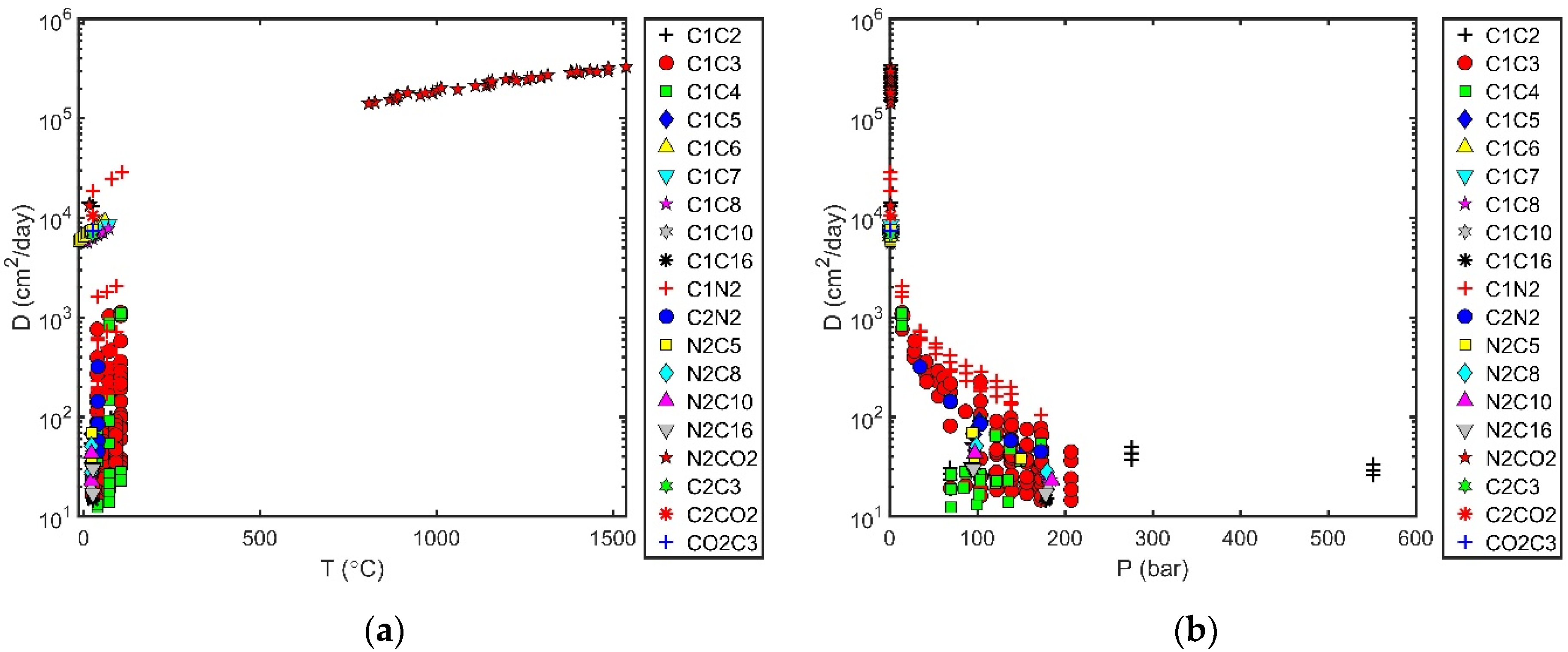
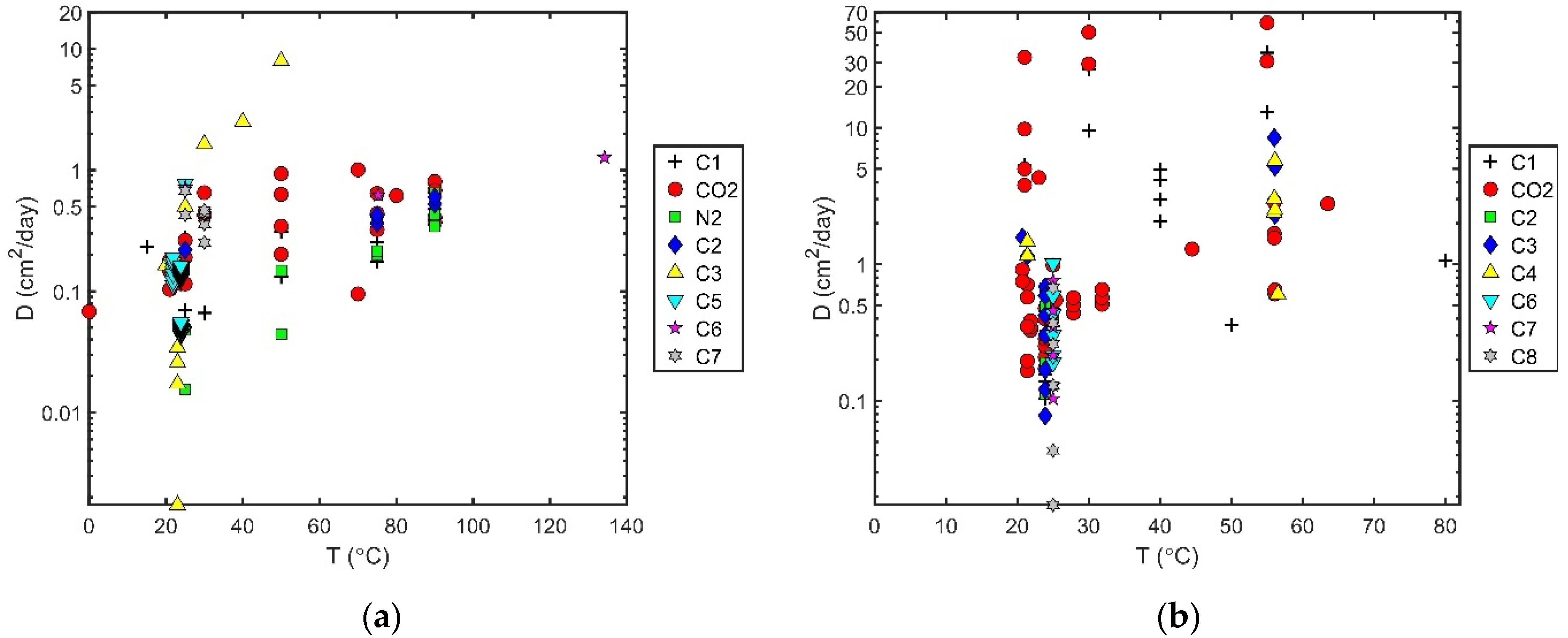
2.3. Trends in Diffusion Coefficients

It is useful to inspect how the diffusion coefficient varies with temperature, pressure, and composition. It not only provides an overview of the data availability in different classes of systems and trends in individual systems, but also helps to identify outliers in the data. Diffusion coefficients for a specific binary pair are functions of temperature, pressure, and composition. It is difficult to visualize the variations of the diffusion coefficients with all the three variables simultaneously. Furthermore, the diffusion data are generally not sufficiently systematic for a simultaneous representation with temperature, pressure, and composition. In the following, we will first show the data for several important classes of systems in plots of diffusion coefficients versus either temperature or pressure—since the composition is not kept constant, the observed trends are just rough ones. Then, we select several systems with relatively systematic data and show the trends with a single variable (temperature, pressure, or composition).

• Trends with temperature or pressure for different classes

Figure 1, Figure 2, Figure 3 and Figure 4 show the diffusion coefficients in several selected classes, including C₁-C_n, CO₂-C_n, C₅/C₆/C₇/C₈-C_n, and gas-phase diffusion coefficients, versus temperature and pressure. Here, C_n is an n-alkane heavier than the other component in the pair.

The C₁-C_n systems are perhaps the most relevant to reservoir fluids. Figure 1 shows the data for ten C₁-C_n systems. The diffusion coefficients are roughly in the range of 0.5–60 cm²/day for the range 0–300 °C and 0–700 bar. The points are denser at lower temperatures and pressures, and they become scarce at higher temperatures and pressures. By inspecting the data at the same temperature or pressure, we can see that the diffusion coefficient decreases with the carbon number of C_n. The systems C₁-C₅, C₁-C₇, C₁-C₁₀, and C₁-C₁₆ have data widely distributed in temperature and pressure. In Figure 1, we can see a clear increasing trend of diffusion coefficient with temperature, as well as a tendency of decreasing diffusion coefficient with pressure. However, it should be noted that, since the composition is not fixed here, the variation in composition affects the observed trends. For temperature whose influence is more dominant than other factors, a clear trend can be observed in Figure 1a. In contrast, it is not easy to judge the trend with pressure from Figure 1b, when the composition varies.

The CO₂-C_n systems are directly related to CO₂ enhanced oil recovery and CO₂ sequestration, thus another important class for reservoir applications. Figure 2 summarizes the data for 12 systems. Most diffusion coefficients are in a range similar to that for C₁-C_n at the same temperature and pressure range. However, there seems to be a larger scattering, with some diffusion coefficients exceptionally high. The CO₂-C₁₆ data measured by Du et al. [125] using PDM are much higher than the others. We consider the data to be outliers and have excluded them from our correlation evaluation. Regarding the variation with C_n, temperature, and pressure, we can again see a decreasing trend with the carbon number and increasing trend with temperature. The trend with pressure is not obvious.

For systems with other gas or light components, including N₂-C_n, C₂-C_n, C₃-C_n, C₄-C_n, and C₁₀/C₁₂/C₁₄/C₁₆-C_n, their figures are presented in the supplementary materials. The trends with the carbon number and temperature were similar.

Figure 3 presents the liquid-phase diffusion coefficients for several light liquid components (C₅, C₆, C₇, and C₈) in C_n. There were 25 systems in total. The selected temperature range was the same as in Figure 1 and Figure 2. The data at high pressures were scarce, and the collected data were all below 40 bar. The diffusion coefficients were smaller than those for gaseous or lighter components. The value was lower than 10 cm²/day for temperatures lower than 100 °C and reached around 20 cm²/day at 300 °C. For heavier liquid components (C₁₀, C₁₂, C₁₄, and C₁₆), their figures for 12 systems are provided in the supplementary materials. The diffusion coefficient was lower than 10 cm²/day, even at temperatures as high as 300 °C. The measured data were limited to low pressures (<15 bar).

Figure 4 summarizes the gas-phase diffusion coefficients for 19 systems in which there is at least one gaseous component (N₂, CO₂, C₁, and C₂). The data covers a wide temperature and pressure range, up to 1500 °C and 550 bar. However, most data were measured below 100 °C and 200 bar. Compared to the liquid-phase diffusion coefficients, the gas-phase diffusion coefficients were more sensitive to pressure. The coefficients decreased with increasing pressure. At pressure lower than 100 bar, the coefficients were generally higher than 100 cm²/day. In the pressure range 100–200 bar, except for C₁-N₂, the other systems had coefficients lower than 100 cm²/day, thus becoming more similar to the typical values of liquid-phase diffusion coefficients. It should be noted that the gas-phase diffusion coefficient generally decreased with pressure, and there seemed to be an exception for high-pressure gas close to the mixture critical point [79], where a reverse trend with pressure was observed.

Figure 5 shows the influence of pressure on the liquid-phase diffusion coefficient for two binaries, C₁-C₇ and CO₂-C₁₆, at fixed compositions. The data at different temperatures are presented. The diffusion coefficient decreased slightly with pressure. At 100 °C, the coefficient for CO₂-C₁₆ decreased from 5.8 to 4.0 cm²/day as the pressure increased from 14 to 670 bar. For C₁-C₇, the diffusion coefficient seemed to be more sensitive to the pressure change. However, there was a larger scattering in the data, making it difficult to quantify the pressure influence. In Figure 1b, the C₁-C₁₀ data seemed to indicate much larger pressure sensitivity. We should bear in mind that the mole fraction also changed with pressure at each isotherm, which provides the illusion of a much larger pressure dependence.

Figure 6 presents two examples for the composition influence: one for the atmospheric liquid-phase diffusion in C₆-C₇ at different temperatures and another for gas-phase diffusion in C₁-C₃ at 105 °C and different pressures. The composition dependence does not show any obvious non-monotonic behavior here. The sensitivity to composition variation was much higher in C₁-C₃ than C₆-C₇. For the gas diffusion in C₁-C₃, the composition variation provided a larger change in the mixture density and viscosity and, thus, a larger change in the diffusion coefficient. Especially at high pressures (138 or 170 bar), the diffusion coefficient was similar to a gaseous one at a high C₁ mole fraction, but similar to a liquid one at a high C₃ mole fraction. In comparison, C₆ and C₇ were alike, and the range of variation was limited.

3. Diffusion Coefficients in Oil Systems

The diffusion data in oil systems were even more scarce in the open literature, due to several reasons. First, petroleum oil is an ill-defined mixture with a large variety in its constituents. Different oils can differ significantly in their composition, thus resulting in different densities, viscosities, and boiling point ranges. Whether the oil is degassed or not also makes a big difference. For such a huge variety of mixtures, it is more common to measure the diffusion coefficients at the most relevant conditions for a particular oil, rather than to carry out a systematic study. Second, the measurement is generally conducted at elevated pressures, even for degassed oil, which increases the experimental difficulty. Third, some measurements are conducted as commercial PVT studies, and the results are not available in the open literature.

To include as many useful data for reservoir fluids as possible, we adopt a broad definition for oil here by including reservoir fluids, degassed oil (such as stock tank oil), and crude oil, as well as products from crude oil (such as kerosene and white oil). In total, we collected 50 papers with measured diffusion coefficients of n-alkane/CO₂/N₂ in the bulk phase of oil. A large number of studies were for heavy oil and bitumen, where diffusion was a crucial mechanism in their production and processing. We, therefore, split the collected data into two groups, heavy and other oils, as presented in Table 3 and Table 4, respectively. These two tables include only degassed oils. The diffusion in live oils [152,153], which are rarely reported, and porous media [154,155,156,157] were excluded.

Table 3 and Table 4 provide systems, data sources, experimental methods, oil viscosities, number of points, and ranges of temperature and pressure. Each system consists of a diffusing component and certain oil sample. Since each oil is unique and provides a long list of systems, although the number of data points for each is often small. These oil samples generally do not have a complete composition description. The oil viscosities, critical to diffusion estimation, were, therefore, included in the tables. In total, there are 215 data points for heavy oils in Table 3, as well as 179 data points for the other oils in Table 4.

The experimental methods used for diffusion measurement in oils are similar to those described in Section 2. In practice, CVD and CP are, so far, the most frequently used methods, with 19 and 13 studies, respectively. The X-ray computer assisted tomography (X-ray CT) method was used in six bitumen studies. By detecting the density variation, it determines the concentration variation during the experimental diffusion process, which is used in data fitting to determine the diffusion coefficients. The method can generate concentration-dependent diffusion coefficients [158,159,160,161,162]. PDM, proposed in 2005 [151], was used in four heavy oil studies. The other methods only had one or two studies. It is worthwhile to mention the recently proposed microfluidic chip method [163,164], which captures the images of the diffusion-driven swelling process on a chip. It can potentially speed up the diffusion measurement, as compared to methods relying on diffusion on a larger scale, such as CVD. In Table 3 and Table 4, we use the same abbreviations for the experimental methods as in Table 2.

The collected diffusion coefficients for the alkane/N₂/CO₂-heavy oil/bitumen systems were in the range of 1–141 bar and 0–134 °C. The solute alkane here covered C₁ to C₈. Most heavy oil and bitumen samples were from Canada. Figure 7 presents the variation of the diffusion coefficients in heavy oils with temperature and pressure. Figure 8 further splits the data into two groups: those in bitumen and those in non-bitumen heavy oil. As shown in Figure 7, the collected diffusion coefficients varied from 0.002 to 58.8 cm²/day. Actually, if we rule out the lowest value and eight high values (9.5 to 58.8 cm²/day) from the same source [165], the range became 0.01 to 10 cm²/day. In fact, 80% of the data lied in the range of 0.01 to 1 cm²/day. Most data (140 points) were measured at the room temperature (<30 °C). There were 51 and 23 points in the range of 30–60 °C and 60–100 °C, respectively. Only one point was at a temperature larger than 100 °C. There were roughly 1/3 data points above 50 °C. The diffusion coefficient generally increases with temperature. However, it can be seen that, at a specific temperature, the coefficient spanned a large range. Regarding the distribution of pressure, 75 points (35%) were at atmospheric pressure, 96 points (34%) above atmospheric pressure, but below 50 bar, 40 points (19%) between 50 and 100 bar; only five points were higher than 100 bar. The highest pressure was 141 bar. No clear pressure dependence can be seen from Figure 7b, since the influences from the other factors (the oil characteristic, solute, and temperature) were more dominant. If we split the oil systems into bitumen and non-bitumen heavy oil, as shown in Figure 8, we can find that most coefficients in bitumen were below 1 cm²/day, whereas those in non-bitumen were generally larger than 0.1 cm²/day, with 50% in the range of 0.1–1 cm²/day and 23% in the range of 1–5 cm²/day. It should be noted that the split between bitumen and non-bitumen was simply based on the description in the original literature but not a rigorous criterion.

The collected diffusion coefficients for the alkanes/N₂/CO₂ + non-heavy oil systems were in the range of 1–347 bar and 4–204 °C. The alkanes included C₁, C₂, and C₃. The group of Guo et al. (2011, 2017) [166,167] reported some of the lowest values, around 0.01 cm²/day. Wang et al. (2013) [168] and Li et al. (2020) [169] reported some large CO₂ diffusion coefficients (11 points) in crude oil, higher than 35 cm²/day, with the maximum reaching 155 cm²/day. Except for these extreme values, most diffusion coefficients were distributed rather evenly in the range of 0.1–20 cm²/day. Figure 9 presents the coefficients versus temperature or pressure. The data ranged from 5 to 205 °C. There were 26%, 39%, 20%, and 16% of data in the range of <30 °C, 30–60 °C, 60–100 °C, and >100 °C, respectively. The increasing trend with temperature can be observed in Figure 9a since temperature provides a dominant influence. The pressure range of the data was 1–347 bar. The data for methane covered the whole pressure range. For the other solutes, the data were mainly below 100 bar. It is difficult to determine the pressure trend from Figure 9b, since the influences from the other factors were stronger.

Table 3. Overview of diffusion coefficients in heavy oils.

System	Visc. (cP)	Method	Np	P (bar)	T (K)	Source
C1 + Bitumen (Athabasca)	-	CVD	3	40–80	298–363	[146]
C1 + Bitumen (Athabasca)	3165	CVD	2	40–80	348	[146]
C1 + Bitumen (Athabasca)	70,475	CVD	1	80	323	[146]
C1 + bitumen (Athabasca)	100,000	CP	1	38	323	[82]
C1 + bitumen (Canadian)	-	CVD	2	34.6–35.9	288–298	[81]
C1 + bitumen (MacKay)	82,160	CVD	1	35.5	303	[170]
C1 + heavy oil	-	CVD	2	63.5–63.9	323–353	[83]
C1 + heavy oil (Lloydminster)	20,267	CVD	1	41.8	297	[171]
C1 + heavy oil (Lloydminster)	23,000	PDM	5	59.6–141.2	297	[172]
C1 + heavy oil (Venezuela)	5000	CVD	1	34.71	294	[173]
C1 + heavy oil sample1	21,285	CVD	2	14	303–328	[165]
C1 + heavy oil sample2	8154	CVD	2	14	303–328	[165]
C1 + heavy oil (Henan)	5824	CP	4	40–100	313	[174]
C2 + Bitumen (Athabasca)	-	CVD	3	40–80	298–363	[146]
C2 + Bitumen (Athabasca)	3165	CVD	2	40–80	348	[146]
C2 + heavy oil (Lloydminster)	23,000	PDM	5	15.2–35	297	[172]
C3 + heavy oil (Lloydminster)	-	CP	1	55.4	329	[175]
C3 + heavy oil (Lloydminster)	-	CP	1	55.4	329	[176]
C3 + heavy oil (Lloydminster)	13,924	CP	1	39.5	294	[177]
C3 + heavy oil (Lloydminster)	-	CP	1	55	329	[176]
C3 + heavy oil (Lloydminster)	12,854	CVD	1	38	295	[178]
C3 + bitumen (Athabasca)	473,000	Microchip	2	6.6–7.5	293–298	[164]
C3 + bitumen (Athabasca)	-	Microchip	3	8.4–13.3	303–323	[164]
C3 + bitumen E2	79,433	X-ray CT	1	6.3	296	[161]
C3 + bitumen L4	501,187	X-ray CT	1	6.3	296	[161]
C3 + bitumen M3	125,893	X-ray CT	1	6.3	296	[161]
C3 + bitumen N1	3162	X-ray CT	1	6.3	296	[161]
C3 + heavy oil (Lloydminster)	20,267	CVD	1	7.6	297	[171]
C3 + heavy oil (Lloydminster)	23,000	PDM	6	4–9	297	[172]
C4 + heavy oil (Lloydminster)	-	CP	1	55.4	329	[175]
C4 + heavy oil (Lloydminster)	-	CP	1	55.4	329	[176]
C4 + heavy oil (Lloydminster)	-	CP	1	55.2	329	[175]
C4 + heavy oil (Lloydminster)	12,854	CP	1	37.4	295	[176]
C4 + heavy oil (Lloydminster)	-	CP	1	55.2	329	[176]
C4 + heavy oil (Lloydminster)	12,854	CVD	1	11.3	295	[178]
C4 + heavy oil (Lloydminster)	-	CP	1	5.3	330	[175]
C5 + bitumen (Athabasca)	18,000	X-ray CT	1	1	295	[158]
C5 + bitumen (Athabasca)	18,000	X-ray CT	17	1	295	[159]
C5 + Bitumen (Cold Lake)	130,000	NMR	1	1	298	[179]
C5 + bitumen 1 (Athabasca)	18,000	X-ray CT	17	1	297	[160]
C5 + bitumen 2 (Athabasca)	2,600,000	X-ray CT	12	1	297	[160]
C6 + bitumen (Athabasca)	-	X-ray CT	2	34.4–35.1	348–407	[162]
C6 + Bitumen (Cold Lake)	130,000	NMR	1	1	298	[179]
C6 + heavy oil	-	X-ray CT	6	1	298	[180]
C7 + bitumen (Atlee Buffalo)	6000	NMR	1	1	298	[179]
C7 + bitumen (Cold Lake)	130,000	NMR	6	1	303	[179]
C7 + bitumen (Peace River)	670,000	NMR	1	1	298	[179]
C7 + heavy oil	-	X-ray CT	6	1	298	[180]
C8 + heavy oil	-	X-ray CT	6	1	298	[180]
CO2 + heavy oil (Lloydminster)	-	CP	1	55.4	329	[175]
CO2 + heavy oil (Lloydminster)	-	CP	1	55.4	329	[176]
CO2 + heavy oil (Lloydminster)	13,924	CP	1	39.5	294	[177]
CO2 + heavy oil (Lloydminster)	-	CP	1	55	329	[176]
CO2 + heavy oil (Lloydminster)	-	CP	1	55.2	329	[175]
CO2 + heavy oil (Lloydminster)	12,854	CP	1	37.4	295	[176]
CO2 + heavy oil (Lloydminster)	-	CP	1	55.2	329	[176]
CO2 + heavy oil (Lloydminster)	12,854	CVD	1	38	295	[178]
CO2 + heavy oil (Lloydminster)	12,854	CVD	1	11.3	295	[178]
CO2 + bitumen	-	CVD	1	48.3	353	[181]
CO2 + bitumen	-	CVD	6	22.4–50.1	303–343	[182]
CO2 + bitumen (Athabasca)	250	CVD	1	40	363	[183]
CO2 + bitumen (Athabasca)	-	CVD	1	40	298	[183]
CO2 + Bitumen (Athabasca)	3165	CVD	2	40–80	348	[146]
CO2 + Bitumen (Athabasca)	70,475	CVD	2	40–80	323	[146]
CO2 + Bitumen (Athabasca)	-	CVD	3	40–80	298–363	[146]
CO2 + bitumen (Athabasca)	10,000	CP	1	32.4	348	[82]
CO2 + bitumen (Athabasca)	2,000,000	other	3	31–56	294	[163]
CO2 + bitumen (Canadian)	-	CVD	2	34.5–34.6	273–298	[81]
CO2 + bitumen (MacKay)	127,868	CVD	1	35.3	297	[170]
CO2 + heavy oil (Aberfeldy)	1058	CP	1	10	296	[184]
CO2 + heavy oil (Lloydminster)	12,854	CVD	1	37.4	295	[178]
CO2 + heavy oil (Lloydminster)	-	CP	1	54	318	[175]
CO2 + heavy oil (Lloydminster)	13,924	CP	1	39.5	294	[177]
CO2 + heavy oil (Lloydminster)	-	CP	3	54	299–337	[185]
CO2 + heavy oil (Lloydminster)	12,854	CP	1	37.4	295	[176]
CO2 + heavy oil (Lloydminster)	20,267	CVD	1	50.3	297	[171]
CO2 + heavy oil (Lloydminster)	23,000	PDM	5	20–60	297	[151]
CO2 + heavy oil (Manatokan)	179	CVD	1	50	294	[186]
CO2 + heavy oil (Ontario)	-	PDM	1	29	298	[187]
CO2 + heavy oil (Venezuela)	5000	CVD	1	35.1	294	[173]
CO2 + heavy oil A (Saskatchewan)	5000	CVD	1	17.3	298	[188]
CO2 + heavy oil A (Saskatchewan)	-	CVD	11	17.2–44.9	295–305	[188]
CO2 + heavy oil 1	21,285	CVD	2	28.5	303–328	[165]
CO2 + heavy oil 2	8154	CVD	2	26	303–328	[165]
N2 + Bitumen (Athabasca)	-	CVD	4	40–80	298–363	[146]
N2 + Bitumen (Athabasca)	3165	CVD	2	40–80	348	[146]
N2 + Bitumen (Athabasca)	70,475	CVD	2	40–80	323	[146]

Table 3. Overview of diffusion coefficients in heavy oils.

System	Visc. (cP)	Method	Np	P (bar)	T (K)	Source
C1 + Bitumen (Athabasca)	-	CVD	3	40–80	298–363	[146]
C1 + Bitumen (Athabasca)	3165	CVD	2	40–80	348	[146]
C1 + Bitumen (Athabasca)	70,475	CVD	1	80	323	[146]
C1 + bitumen (Athabasca)	100,000	CP	1	38	323	[82]
C1 + bitumen (Canadian)	-	CVD	2	34.6–35.9	288–298	[81]
C1 + bitumen (MacKay)	82,160	CVD	1	35.5	303	[170]
C1 + heavy oil	-	CVD	2	63.5–63.9	323–353	[83]
C1 + heavy oil (Lloydminster)	20,267	CVD	1	41.8	297	[171]
C1 + heavy oil (Lloydminster)	23,000	PDM	5	59.6–141.2	297	[172]
C1 + heavy oil (Venezuela)	5000	CVD	1	34.71	294	[173]
C1 + heavy oil sample1	21,285	CVD	2	14	303–328	[165]
C1 + heavy oil sample2	8154	CVD	2	14	303–328	[165]
C1 + heavy oil (Henan)	5824	CP	4	40–100	313	[174]
C2 + Bitumen (Athabasca)	-	CVD	3	40–80	298–363	[146]
C2 + Bitumen (Athabasca)	3165	CVD	2	40–80	348	[146]
C2 + heavy oil (Lloydminster)	23,000	PDM	5	15.2–35	297	[172]
C3 + heavy oil (Lloydminster)	-	CP	1	55.4	329	[175]
C3 + heavy oil (Lloydminster)	-	CP	1	55.4	329	[176]
C3 + heavy oil (Lloydminster)	13,924	CP	1	39.5	294	[177]
C3 + heavy oil (Lloydminster)	-	CP	1	55	329	[176]
C3 + heavy oil (Lloydminster)	12,854	CVD	1	38	295	[178]
C3 + bitumen (Athabasca)	473,000	Microchip	2	6.6–7.5	293–298	[164]
C3 + bitumen (Athabasca)	-	Microchip	3	8.4–13.3	303–323	[164]
C3 + bitumen E2	79,433	X-ray CT	1	6.3	296	[161]
C3 + bitumen L4	501,187	X-ray CT	1	6.3	296	[161]
C3 + bitumen M3	125,893	X-ray CT	1	6.3	296	[161]
C3 + bitumen N1	3162	X-ray CT	1	6.3	296	[161]
C3 + heavy oil (Lloydminster)	20,267	CVD	1	7.6	297	[171]
C3 + heavy oil (Lloydminster)	23,000	PDM	6	4–9	297	[172]
C4 + heavy oil (Lloydminster)	-	CP	1	55.4	329	[175]
C4 + heavy oil (Lloydminster)	-	CP	1	55.4	329	[176]
C4 + heavy oil (Lloydminster)	-	CP	1	55.2	329	[175]
C4 + heavy oil (Lloydminster)	12,854	CP	1	37.4	295	[176]
C4 + heavy oil (Lloydminster)	-	CP	1	55.2	329	[176]
C4 + heavy oil (Lloydminster)	12,854	CVD	1	11.3	295	[178]
C4 + heavy oil (Lloydminster)	-	CP	1	5.3	330	[175]
C5 + bitumen (Athabasca)	18,000	X-ray CT	1	1	295	[158]
C5 + bitumen (Athabasca)	18,000	X-ray CT	17	1	295	[159]
C5 + Bitumen (Cold Lake)	130,000	NMR	1	1	298	[179]
C5 + bitumen 1 (Athabasca)	18,000	X-ray CT	17	1	297	[160]
C5 + bitumen 2 (Athabasca)	2,600,000	X-ray CT	12	1	297	[160]
C6 + bitumen (Athabasca)	-	X-ray CT	2	34.4–35.1	348–407	[162]
C6 + Bitumen (Cold Lake)	130,000	NMR	1	1	298	[179]
C6 + heavy oil	-	X-ray CT	6	1	298	[180]
C7 + bitumen (Atlee Buffalo)	6000	NMR	1	1	298	[179]
C7 + bitumen (Cold Lake)	130,000	NMR	6	1	303	[179]
C7 + bitumen (Peace River)	670,000	NMR	1	1	298	[179]
C7 + heavy oil	-	X-ray CT	6	1	298	[180]
C8 + heavy oil	-	X-ray CT	6	1	298	[180]
CO2 + heavy oil (Lloydminster)	-	CP	1	55.4	329	[175]
CO2 + heavy oil (Lloydminster)	-	CP	1	55.4	329	[176]
CO2 + heavy oil (Lloydminster)	13,924	CP	1	39.5	294	[177]
CO2 + heavy oil (Lloydminster)	-	CP	1	55	329	[176]
CO2 + heavy oil (Lloydminster)	-	CP	1	55.2	329	[175]
CO2 + heavy oil (Lloydminster)	12,854	CP	1	37.4	295	[176]
CO2 + heavy oil (Lloydminster)	-	CP	1	55.2	329	[176]
CO2 + heavy oil (Lloydminster)	12,854	CVD	1	38	295	[178]
CO2 + heavy oil (Lloydminster)	12,854	CVD	1	11.3	295	[178]
CO2 + bitumen	-	CVD	1	48.3	353	[181]
CO2 + bitumen	-	CVD	6	22.4–50.1	303–343	[182]
CO2 + bitumen (Athabasca)	250	CVD	1	40	363	[183]
CO2 + bitumen (Athabasca)	-	CVD	1	40	298	[183]
CO2 + Bitumen (Athabasca)	3165	CVD	2	40–80	348	[146]
CO2 + Bitumen (Athabasca)	70,475	CVD	2	40–80	323	[146]
CO2 + Bitumen (Athabasca)	-	CVD	3	40–80	298–363	[146]
CO2 + bitumen (Athabasca)	10,000	CP	1	32.4	348	[82]
CO2 + bitumen (Athabasca)	2,000,000	other	3	31–56	294	[163]
CO2 + bitumen (Canadian)	-	CVD	2	34.5–34.6	273–298	[81]
CO2 + bitumen (MacKay)	127,868	CVD	1	35.3	297	[170]
CO2 + heavy oil (Aberfeldy)	1058	CP	1	10	296	[184]
CO2 + heavy oil (Lloydminster)	12,854	CVD	1	37.4	295	[178]
CO2 + heavy oil (Lloydminster)	-	CP	1	54	318	[175]
CO2 + heavy oil (Lloydminster)	13,924	CP	1	39.5	294	[177]
CO2 + heavy oil (Lloydminster)	-	CP	3	54	299–337	[185]
CO2 + heavy oil (Lloydminster)	12,854	CP	1	37.4	295	[176]
CO2 + heavy oil (Lloydminster)	20,267	CVD	1	50.3	297	[171]
CO2 + heavy oil (Lloydminster)	23,000	PDM	5	20–60	297	[151]
CO2 + heavy oil (Manatokan)	179	CVD	1	50	294	[186]
CO2 + heavy oil (Ontario)	-	PDM	1	29	298	[187]
CO2 + heavy oil (Venezuela)	5000	CVD	1	35.1	294	[173]
CO2 + heavy oil A (Saskatchewan)	5000	CVD	1	17.3	298	[188]
CO2 + heavy oil A (Saskatchewan)	-	CVD	11	17.2–44.9	295–305	[188]
CO2 + heavy oil 1	21,285	CVD	2	28.5	303–328	[165]
CO2 + heavy oil 2	8154	CVD	2	26	303–328	[165]
N2 + Bitumen (Athabasca)	-	CVD	4	40–80	298–363	[146]
N2 + Bitumen (Athabasca)	3165	CVD	2	40–80	348	[146]
N2 + Bitumen (Athabasca)	70,475	CVD	2	40–80	323	[146]

Table 4. Overview of diffusion coefficients in other oils.

System	Visc. (cP)	Method	Np	P (bar)	T (K)	Source
C1 + crude oil	-	CVD	3	200	333	[166]
C1 + crude oil (Bakken)	-	CVD	1	137.9	294	[189]
C1 + crude oil (Sante Fe Springs)	-	CP	19	23.4–286.7	278–411	[190]
C1 + crude oil (typical Iranian)	-	CP	16	35–275	298–323	[80]
C1 + white oil	3.8	CP	5	37.8–330.5	378	[191]
C1 + white oil	-	CP	15	35.4–347.2	278–444	[191]
C1 + condensate oil	-	CVD	1	200	333	[167]
C2 + crude oil	4.1	CVD	1	35.5	353	[192]
C2 + white oil	3.8	CP	4	9.8–76.8	378	[193]
C2 + white oil	-	CP	14	5.5–41.4	278–478	[193]
C3 + kerosene	0.9	CP	5	2.1–13.9	333	[194]
C3 + kerosene	1.2	CP	3	1.8–10.3	318	[194]
C3 + kerosene	1.4	CP	11	2.1–7.2	303	[194]
C3 + spray oil	5.1	CP	4	2.2–14	333	[194]
C3 + spray oil	7.9	CP	4	1.8–9.1	318	[194]
C3 + spray oil	13.5	CP	4	2.2–7.2	303	[194]
CO2 + light oil (Bakken)	-	CP	1	21.7	336	[195]
CO2 + crude oil	-	CVD	3	200	333	[166]
CO2 + crude oil (Maljamar)	-	HCT	1	52.1	298	[114]
CO2 + crude oil (Shengli)	151.0	CVD	3	39.3–142.8	323	[169]
CO2 + crude oil (Weyburn)	-	PDM	5	3.2–43.9	300	[196]
CO2 + crude oil (Daqing)	-	CVD	8	32–82.8	318	[168]
CO2 + gas oil BP 200–300	3.9	other	1	1	298	[119]
CO2 + gas oil BP 300–400	26.5	other	1	1	298	[119]
CO2 + kerosine	1.8	other	1	1	298	[119]
CO2 + white oil no. 15	135.0	other	1	1	298	[197]
CO2 + white oil no. 7	56.0	other	1	1	298	[197]
CO2 + crude oil (Shengli))	151.0	CVD	3	49.8–145.9	323	[169]
CO2 + condensate oil	-	CVD	1	200	333	[167]
CO2 + crude oil (Bakken)	2.2	CVD	4	165.6–210.8	293	[198]
CO2 + crude oil (Bakken)	-	CVD	3	185.2–187.9	313	[198]
N2 + light oil (Bakken)	-	CP	1	52.8	336	[195]
N2 + crude oil	-	CVD	2	200	333	[166]
N2 + RP-3 jet fuel	-	IF	14	1	278–343	[199]
N2 + RP-5 jet fuel	-	IF	14	1	278–343	[199]
N2 + condensate oil	-	CVD	1	200	333	[167]

Table 4. Overview of diffusion coefficients in other oils.

System	Visc. (cP)	Method	Np	P (bar)	T (K)	Source
C1 + crude oil	-	CVD	3	200	333	[166]
C1 + crude oil (Bakken)	-	CVD	1	137.9	294	[189]
C1 + crude oil (Sante Fe Springs)	-	CP	19	23.4–286.7	278–411	[190]
C1 + crude oil (typical Iranian)	-	CP	16	35–275	298–323	[80]
C1 + white oil	3.8	CP	5	37.8–330.5	378	[191]
C1 + white oil	-	CP	15	35.4–347.2	278–444	[191]
C1 + condensate oil	-	CVD	1	200	333	[167]
C2 + crude oil	4.1	CVD	1	35.5	353	[192]
C2 + white oil	3.8	CP	4	9.8–76.8	378	[193]
C2 + white oil	-	CP	14	5.5–41.4	278–478	[193]
C3 + kerosene	0.9	CP	5	2.1–13.9	333	[194]
C3 + kerosene	1.2	CP	3	1.8–10.3	318	[194]
C3 + kerosene	1.4	CP	11	2.1–7.2	303	[194]
C3 + spray oil	5.1	CP	4	2.2–14	333	[194]
C3 + spray oil	7.9	CP	4	1.8–9.1	318	[194]
C3 + spray oil	13.5	CP	4	2.2–7.2	303	[194]
CO2 + light oil (Bakken)	-	CP	1	21.7	336	[195]
CO2 + crude oil	-	CVD	3	200	333	[166]
CO2 + crude oil (Maljamar)	-	HCT	1	52.1	298	[114]
CO2 + crude oil (Shengli)	151.0	CVD	3	39.3–142.8	323	[169]
CO2 + crude oil (Weyburn)	-	PDM	5	3.2–43.9	300	[196]
CO2 + crude oil (Daqing)	-	CVD	8	32–82.8	318	[168]
CO2 + gas oil BP 200–300	3.9	other	1	1	298	[119]
CO2 + gas oil BP 300–400	26.5	other	1	1	298	[119]
CO2 + kerosine	1.8	other	1	1	298	[119]
CO2 + white oil no. 15	135.0	other	1	1	298	[197]
CO2 + white oil no. 7	56.0	other	1	1	298	[197]
CO2 + crude oil (Shengli))	151.0	CVD	3	49.8–145.9	323	[169]
CO2 + condensate oil	-	CVD	1	200	333	[167]
CO2 + crude oil (Bakken)	2.2	CVD	4	165.6–210.8	293	[198]
CO2 + crude oil (Bakken)	-	CVD	3	185.2–187.9	313	[198]
N2 + light oil (Bakken)	-	CP	1	52.8	336	[195]
N2 + crude oil	-	CVD	2	200	333	[166]
N2 + RP-3 jet fuel	-	IF	14	1	278–343	[199]
N2 + RP-5 jet fuel	-	IF	14	1	278–343	[199]
N2 + condensate oil	-	CVD	1	200	333	[167]

4. Diffusion Coefficient Correlations

Five diffusion coefficient correlations, including WC [42], HM [43], ES [11,57], RW [47], and LDF [29], were studied here. Among them, WC and HM were based on the Stokes–Einstein theory for liquid viscosity, and the other three shared certain similarities in their forms. We briefly describe their forms and features below.

4.1. Wilke–Chang (WC) Correlation (1955)

The WC correlation was originally designed for low-concentration solute A in solvent B. It is an empirical modification of the Stokes–Einstein relation:

$${\mathrm{D}}_{\mathrm{A}\mathrm{B}}^{\mathrm{o}}=\frac{7.4\times {10}^{-8}{(\Phi {\mathrm{M}}_{\mathrm{B}})}^{1/2}\mathrm{T}}{{\mathsf{\eta }}_{\mathrm{B}}{\mathrm{V}}_{\mathrm{A}}^{0.6}}$$

(1)

where ${\mathrm{D}}_{\mathrm{A}\mathrm{B}}^{\mathrm{o}}$ is the mutual diffusion coefficient (cm²/s) of solute A at very low concentrations in solvent B, M_B is the molecular weight (g/mol) of solvent B, T is temperature (K), Ƞ_B is the viscosity (cP) of solvent B, V_A is the molar volume (cm³/mol) of solute A at its normal boiling temperature, and Φ is the association factor (dimensionless) of solvent B. For the non-associating systems investigated here, Φ was always equal to 1. V_A was estimated from the NIST data whenever possible. If not available, they were estimated by the Tyn and Calus correlation [200].

WC is, in principle, only applicable to dilute regions. There was no consensus on how it should be used to estimate the diffusion coefficient of a mixture whose solute concentration was non-negligible. One can interpret Ƞ_B and M_B as the properties of the mixture solution to partly account for the composition effect. There is, however, still the issue regarding which component is taken as the solute or solvent. For the binary systems in this study, we selected the component with the smaller mole fraction as solute, with the other selected as the solvent. Apparently, this caused a discontinuity at x_A = x_B = 0.5. This inconsistency was inherent in the original correlation.

4.2. Hayduk–Minhas (HM) Correlation (1982)

Hayduk and Minhas proposed new set of correlations for liquid diffusivities, similar to WC in 1982. The proposed correlations are, in principle, only applicable to the infinite dilution binary diffusion coefficients. The following correlation was developed based on normal paraffin solutions and generally recommended for hydrocarbons:

$${\mathrm{D}}_{\mathrm{A}\mathrm{B}}^{\mathrm{o}}=\frac{13.3\times {10}^{-8}{\mathrm{T}}^{1.47}{\mathsf{\eta }}_{\mathrm{B}}{}^{\left(\frac{10.2}{{\mathrm{V}}_{\mathrm{A}}}-0.791\right)}}{{\mathrm{V}}_{\mathrm{A}}^{0.71}}$$

(2)

The symbols in the above HM correlation have the same meaning as in WC. Compared to WC, HM does not require M_B. It has the same inconsistency problem as WC.

4.3. Extended Sigmund (ES) Correlation (1976, 1989)

Sigmund developed, in 1976, a correlation for the binary diffusion coefficients D_ij based on the corresponding states principle. He expressed the ratio of molar density-diffusivity product, ${\mathsf{\rho }}_{\mathrm{M}}{\mathrm{D}}_{\mathrm{i}\mathrm{j}}/{\mathsf{\rho }}_{\mathrm{M}}^{\mathrm{o}}{\mathrm{D}}_{\mathrm{i}\mathrm{j}}^{\mathrm{o}}$, as a polynomial in the pseudo-reduced molar density ρ_pr:

$$\frac{{\mathsf{\rho }}_{\mathrm{M}}{\mathrm{D}}_{\mathrm{i}\mathrm{j}}}{{\mathsf{\rho }}_{\mathrm{M}}^{\mathrm{o}}{\mathrm{D}}_{\mathrm{i}\mathrm{j}}^{\mathrm{o}}}=0.99589+0.096016{\mathsf{\rho }}_{\mathrm{p}\mathrm{r}}-0.22035{\mathsf{\rho }}_{\mathrm{p}\mathrm{r}}^2+0.032874{\mathsf{\rho }}_{\mathrm{p}\mathrm{r}}^3$$

(3)

In the equation, the molar density ρ_M (mol/cm³) and binary diffusion coefficient D_ij (cm²/s) were at the system temperature and pressure. ρ_pr is calculated as ρ_M/ρ_c, where ρ_c is the mixture pseudo-critical molar density (mol/cm³), given by

$${\mathsf{\rho }}_{\mathrm{c}}=\frac{{\displaystyle \sum _{}^{}{\mathrm{x}}_{\mathrm{i}}{\mathrm{v}}_{\mathrm{c}\mathrm{i}}{}^{2/3}}}{{\displaystyle \sum _{}^{}{\mathrm{x}}_{\mathrm{i}}{\mathrm{v}}_{\mathrm{c}\mathrm{i}}{}^{5/3}}}$$

(4)

with v_ci being the critical molar volume (cm³/mol) and x_i being the mole fraction of component i. The low-pressure density-diffusivity product ${\mathsf{\rho }}_{\mathrm{M}}^{\mathrm{o}}{\mathrm{D}}_{\mathrm{i}\mathrm{j}}^{\mathrm{o}}$ is a function of temperature and composition only, and it can be calculated using the Chapman–Enskog dilute gas theory [201]:

$${\mathsf{\rho }}_{\mathrm{M}}^{\mathrm{o}}{\mathrm{D}}_{\mathrm{i}\mathrm{j}}^{\mathrm{o}}=\frac{2.2648\times {10}^{-5}}{{\mathsf{\sigma }}_{\mathrm{i}\mathrm{j}}^2{\mathsf{\Omega }}_{\mathrm{i}\mathrm{j}}}\sqrt{\mathrm{T}\left(\frac{1}{{\mathrm{M}}_{\mathrm{i}}}+\frac{1}{{\mathrm{M}}_{\mathrm{j}}}\right)}$$

(5)

where T is the temperature (K), M_i is the molecular weight (g/mol), σ is the Lennard–Jones 12-6 collision diameter (Å), and Ω_ij is the binary diffusion collision integral (dimensionless) given by:

$${\mathsf{\Omega }}_{\mathrm{i}\mathrm{j}}=\frac{1.06036}{{\mathrm{T}}_{\mathrm{i}\mathrm{j}}^{0.1561}}+\frac{0.193}{\mathrm{e}\mathrm{x}\mathrm{p}(0.47635{\mathrm{T}}_{\mathrm{i}\mathrm{j}})}+\frac{1.03587}{\mathrm{e}\mathrm{x}\mathrm{p}(1.52996{\mathrm{T}}_{\mathrm{i}\mathrm{j}})}+\frac{1.76474}{\mathrm{e}\mathrm{x}\mathrm{p}(3.89411{\mathrm{T}}_{\mathrm{i}\mathrm{j}})}$$

(6)

where T_ij = T/(ε/κ)_ij, ε is the Lennard–Jones 12-6 potential energy parameter (J), and κ is the Boltzmann parameter. The cross parameters σ_ij and ε_ij were calculated from the pure component parameters σ_i and ε_i, using the following combining rules:

$${\mathsf{\sigma }}_{\mathrm{i}\mathrm{j}}=\frac{{\mathsf{\sigma }}_{\mathrm{i}}+{\mathsf{\sigma }}_{\mathrm{j}}}{2}$$

(7)

$${\left(\frac{\mathsf{\epsilon }}{\mathsf{\kappa }}\right)}_{\mathrm{i}\mathrm{j}}=\sqrt{{\left(\frac{\mathsf{\epsilon }}{\mathsf{\kappa }}\right)}_{\mathrm{i}}{\left(\frac{\mathsf{\epsilon }}{\mathsf{\kappa }}\right)}_{\mathrm{j}}}$$

(8)

with

$${\mathsf{\sigma }}_{\mathrm{i}}=0.1866\frac{{\mathrm{v}}_{\mathrm{c}\mathrm{i}}^{1/3}}{{\mathrm{z}}_{\mathrm{c}\mathrm{i}}^{6/5}}$$

(9)

$${\left(\frac{\mathsf{\epsilon }}{\mathsf{\kappa }}\right)}_{\mathrm{i}}=65.3{\mathrm{T}}_{\mathrm{c}\mathrm{i}}{\mathrm{z}}_{\mathrm{c}\mathrm{i}}^{18/5}$$

(10)

where z_ci is the critical compressibility factor.

Da Silva and Belery, in 1989, devised a small modification of the Sigmund correlation. They noticed that Equation (3) provides negative diffusion coefficients at high ρ_pr and suggested using the equation only for ρ_pr ≤ 3. For ρ_pr > 3, they proposed the following modification:

$$\frac{{\mathsf{\rho }}_{\mathrm{M}}{\mathrm{D}}_{\mathrm{i}\mathrm{j}}}{{\mathsf{\rho }}_{\mathrm{M}}^{\mathrm{o}}{\mathrm{D}}_{\mathrm{i}\mathrm{j}}^{\mathrm{o}}}=0.18839\mathrm{e}\mathrm{x}\mathrm{p}(3-{\mathsf{\rho }}_{\mathrm{p}\mathrm{r}})$$

(11)

However, they did not provide the details regarding how Equation (11) was developed, e.g., what data were used in regressing the correlation. Equation (3) together with (11) are known as the extended Sigmund (ES) correlation.

ES was originally developed using the binary dense-gas diffusion data and binary Fickian law. In order to apply the correlation to multicomponent mixtures, we can use the Wilke equation (1950) [202] to calculate the effective diffusion coefficients D_im from D_ij:

$${\mathrm{D}}_{\mathrm{i}\mathrm{m}}=\frac{1-{\mathrm{x}}_{\mathrm{i}}}{{\displaystyle \sum _{\mathrm{j}\ne \mathrm{i}}^{}{\mathrm{x}}_{\mathrm{j}}/{\mathrm{D}}_{\mathrm{i}\mathrm{j}}}}$$

(12)

Note that the Wilke equation was developed under the Maxwell–Stefan (MS) framework. Using Equation (12) essentially assumes that the D_ij from ES can be treated as the MS diffusion coefficients. For a mixture with N_c components, ES gives N_c(N_c − 1)/2 D_ij, and the D matrix is symmetric (D_ij = D_ji). The MS diffusion coefficients also share these two features. In contrast, the Fickian diffusion coefficients have (N_c − 1)² independent values, and its D matrix is not symmetric. Nevertheless, substituting the Sigmund D_ij directly to the Wilke equation is only an approximation.

4.4. Riazi-Whitson (RW) Correlation (1993)

Riazi and Whitson, in 1993, developed a correlation to estimate diffusion coefficients of dense gases and liquids for both binary and multicomponent systems. Its development has used the ideas from both hydrodynamic theory (using viscosity) [36] and the kinetic theory of gases (using density) [56]. The correlation for a binary mixture is given by:

$$\frac{{\mathsf{\rho }}_{\mathrm{M}}{\mathrm{D}}_{\mathrm{A}\mathrm{B}}}{{\mathsf{\rho }}_{\mathrm{M}}^{\mathrm{o}}{\mathrm{D}}_{\mathrm{A}\mathrm{B}}^{\mathrm{o}}}=\mathrm{a}{\left(\frac{\mathsf{\mu }}{{\mathsf{\mu }}^{\mathrm{o}}}\right)}^{\mathrm{b}+\mathrm{c}{\mathrm{P}}_{\mathrm{r}}}$$

(13)

where ${\mathsf{\rho }}_{\mathrm{M}}{\mathrm{D}}_{\mathrm{A}\mathrm{B}}$ and ${\mathsf{\rho }}_{\mathrm{M}}^{\mathrm{o}}{\mathrm{D}}_{\mathrm{A}\mathrm{B}}^{\mathrm{o}}$ are the density-diffusivity product at the system conditions and low pressure, respectively. The molar density ρ is in mol/cm³, and the binary diffusion coefficient in cm²/s. As in ES, ${\mathsf{\rho }}_{\mathrm{M}}^{\mathrm{o}}{\mathrm{D}}_{\mathrm{A}\mathrm{B}}^{\mathrm{o}}$ is calculated from the Chapman–Enskog dilute gas theory. The coefficients a, b, and c in Equation (13) are given by

$$\mathrm{a}=1.07$$

(14)

$$\mathrm{b}=-0.27-0.38\mathsf{\omega }$$

(15)

$$\mathrm{c}=-0.05+0.1\mathsf{\omega }$$

(16)

The reduced pressure P_r is calculated given by

$${\mathrm{P}}_{\mathrm{r}}=\mathrm{P}/{\mathrm{P}}_{\mathrm{c}}$$

(17)

The mixture critical pressure P_c and acentric factor ω are calculated by the linear mixing rules:

$${\mathrm{P}}_{\mathrm{c}}={\mathrm{x}}_{\mathrm{A}}{\mathrm{P}}_{\mathrm{c},\mathrm{A}}+{\mathrm{x}}_{\mathrm{B}}{\mathrm{P}}_{\mathrm{c},\mathrm{B}}$$

(18)

$$\mathsf{\omega }={\mathrm{x}}_{\mathrm{A}}{\mathsf{\omega }}_{\mathrm{A}}+{\mathrm{x}}_{\mathrm{B}}{\mathsf{\omega }}_{\mathrm{B}}$$

(19)

with x_A and x_B being the mole fractions of A and B, respectively. The low-pressure mixture viscosity μ^o was estimated from the Stiel and Thodos correlation [203], with the viscosity at the system conditions μ from the generalized Jossi-Stiel-Thodos (1962) correlation [204]. This approach to estimate viscosity is essentially the same as what Lohrenz et al. proposed for the viscosity of reservoir fluids. It is usually called the Lohrenz–Bray–Clark (LBC) correlation in the petroleum engineering area.

Riazi and Whitson discussed how to extend their correlation to multicomponent systems. They proposed to treat the multicomponent mixture as a binary mixture. For an N-component mixture where we want to calculate the effective diffusion coefficient of component A in the mixture, we can treat the other components as one pseudo-component B. Another possible approach, although not discussed by Riazi and Whitson, is to assume Equation (12) is applicable to the D_ij calculation as in ES. Once all the D_ij are calculated, we can use the Wilke equation to estimate the effective diffusion coefficient. We adopted the second method here for multicomponent mixtures.

4.5. Leahy-Dios and Firoozabadi (LDF) Correlation (2007)

Among the correlations discussed here, the LDF correlation is the only one explicitly using the MS framework. The correlation can estimate the MS diffusion coefficients, as well as the generalized Fickian diffusion coefficients and for nonideal and nonpolar multicomponent mixtures. Leahy-Dios and Firoozabadi’s approach was to develop the correlations for infinite dilution diffusion coefficients first, calculate the MS diffusion coefficients using these infinite dilution coefficients, and finally, convert the MS diffusion coefficients to the Fickian ones with the help of a thermodynamic model.

Their correlation for the infinite dilution diffusion coefficients bears certain similarity to ES and the RW, especially to the latter:

$$\frac{\mathrm{c}{\mathrm{D}}_{21}^{\infty }}{{(\mathrm{c}\mathrm{D})}^{\mathrm{o}}}={\mathrm{A}}_0{\left(\frac{{\mathrm{T}}_{\mathrm{r},1}{\mathrm{P}}_{\mathrm{r},2}}{{\mathrm{T}}_{\mathrm{r},2}{\mathrm{P}}_{\mathrm{r},1}}\right)}^{{\mathrm{A}}_1}{\left(\frac{\mathsf{\mu }}{{\mathsf{\mu }}^{\mathrm{o}}}\right)}^{\left[{\mathrm{A}}_2\left({\mathsf{\omega }}_1,{\mathsf{\omega }}_2\right)+{\mathrm{A}}_3\left({\mathrm{P}}_{\mathrm{r}},{\mathrm{T}}_{\mathrm{r}}\right)\right]}$$

(20)

The ratio of the density-diffusivity product $\mathrm{c}{\mathrm{D}}_{21}^{\infty }/{(\mathrm{c}\mathrm{D})}^{\mathrm{o}}$ is expressed as a function of the viscosity ratio ($\mathsf{\mu }/{\mathsf{\mu }}^{\mathrm{o}}$), reduced temperatures T_r,i, pressures P_r,i, and acentric factors ω_i. Different from ES and RW, the molar density c and viscosity μ are for the solvent component 1, instead of the mixture at the system temperature and pressure, and ${\mathrm{D}}_{21}^{\infty }$ is the infinite-dilution diffusion coefficient of component 2 in component 1, instead of the D at the given composition. (cD)^o is the dilute gas density-diffusivity product, which can, in principle, be calculated by the Chapman–Enskog dilute gas theory, as in ES and RW, but Leahy-Dios and Firoozabadi suggested using the approach of Fuller et al. [205]:

$${(\mathrm{c}\mathrm{D})}^{\mathrm{o}}=1.01\times {10}^{-2}{\mathrm{T}}^{0.75}\frac{{\left(\frac{1}{{\mathrm{M}}_1}+\frac{1}{{\mathrm{M}}_2}\right)}^{0.5}}{\mathrm{R}{\left[{\left({\displaystyle \sum {\mathrm{v}}_1}\right)}^{1/3}+{\left({\displaystyle \sum {\mathrm{v}}_2}\right)}^{1/3}\right]}^2}$$

(21)

where M₁ and M₂ are the molar masses (g/mol) of components 1 and 2, respectively. ${\displaystyle \sum {\mathrm{v}}_{\mathrm{i}}}$ is the so-called “diffusion volume increments” of component i, and can be calculated by summing the atomic diffusion volumes [1]. The dilute gas viscosity μ^o was calculated by the Stiel and Thodos correlation:

$$\begin{array}{ll}{\mathsf{\mu }}_{\mathrm{i}}^{\mathrm{o}}{\mathsf{\xi }}_{\mathrm{i}}=34.0\times {10}^{-5}{({\mathrm{T}}_{\mathrm{r},\mathrm{i}})}^{0.94}& \mathrm{f}\mathrm{o}\mathrm{r} {\mathrm{T}}_{\mathrm{r},\mathrm{i}}\le 1.50\\ {\mathsf{\mu }}_{\mathrm{i}}^{\mathrm{o}}{\mathsf{\xi }}_{\mathrm{i}}=17.78\times {10}^{-5}{(4.58{\mathrm{T}}_{\mathrm{r},\mathrm{i}}-1.67)}^{5/8}& \mathrm{f}\mathrm{o}\mathrm{r} {\mathrm{T}}_{\mathrm{r},\mathrm{i}}>1.50\end{array}$$

(22)

with ${\mathsf{\xi }}_{\mathrm{i}}={\mathrm{T}}_{\mathrm{c},\mathrm{i}}{}^{1/6}/\left[{\mathrm{M}}_{\mathrm{i}}{}^{1/2}{(0.987{\mathrm{P}}_{\mathrm{c},\mathrm{i}})}^{2/3}\right]$. They chose the equimolar composition of components 1 and 2 to calculate the reference dilute gas viscosity μ^o:

$${\mathsf{\mu }}^{\mathrm{o}}=\frac{{\mathsf{\mu }}_1^{\mathrm{o}}{\mathrm{M}}_1^{1/2}+{\mathsf{\mu }}_2^{\mathrm{o}}{\mathrm{M}}_2^{1/2}}{{\mathrm{M}}_1^{1/2}+{\mathrm{M}}_2^{1/2}}$$

(23)

The constants A₀ to A₃ in Equation (20) are given by

$${\mathrm{A}}_0={\mathrm{e}}^{{\mathrm{a}}_1}$$

(24)

$${\mathrm{A}}_1=10{\mathrm{a}}_2$$

(25)

$${\mathrm{A}}_2={\mathrm{a}}_3(1+10{\mathsf{\omega }}_1-{\mathsf{\omega }}_2+10{\mathsf{\omega }}_1{\mathsf{\omega }}_2)$$

(26)

$${\mathrm{A}}_3={\mathrm{a}}_4\left({\mathrm{P}}_{\mathrm{r},1}^{3{\mathrm{a}}_5}-6{\mathrm{P}}_{\mathrm{r},2}^{{\mathrm{a}}_5}+6{\mathrm{T}}_{\mathrm{r},1}^{10{\mathrm{a}}_6}\right)+{\mathrm{a}}_7{\mathrm{T}}_{\mathrm{r},2}^{-{\mathrm{a}}_6}+{\mathrm{a}}_2\left(\frac{{\mathrm{T}}_{\mathrm{r},1}{\mathrm{P}}_{\mathrm{r},2}}{{\mathrm{T}}_{\mathrm{r},2}{\mathrm{P}}_{\mathrm{r},1}}\right)$$

(27)

with a₁ = −0.0472, a₂ = 0.0103, a₃ = −0.0147, a₄ = −0.0053, a₅ = −0.3370, a₆ = −0.1852, and a₇ = −0.1914. T_r,I = T/T_c,i and P_r,i = P/P_c,i are the reduced temperature and pressure of component i, respectively.

Leahy-Dios and Firoozabadi did not suggest a single set of models for c and μ. In their development of Equation (20), they used experimental data whenever available; for hydrocarbons, they used the corresponding state theory [206] for μ and PR-EoS with volume translation for c.

Once the infinite-dilution diffusion coefficients for each pair of the components in the mixture ${\mathrm{D}}_{\mathrm{i}\mathrm{j}}^{\infty }$ were estimated, we can estimate the MS diffusion coefficients ${\mathsf{Ð}}_{\mathrm{i}\mathrm{j}}$ at the desired composition using the generalized Vignes relation:

$${\mathsf{Ð}}_{\mathrm{i}\mathrm{j}}={\left({\mathrm{D}}_{\mathrm{i}\mathrm{j}}^{\infty }\right)}^{{\mathrm{x}}_{\mathrm{j}}}{\left({\mathrm{D}}_{\mathrm{j}\mathrm{i}}^{\infty }\right)}^{{\mathrm{x}}_{\mathrm{i}}}{\displaystyle \prod _{\begin{array}{l}\mathrm{k}=1\\ \mathrm{k}\ne \mathrm{i},\mathrm{j}\end{array}}^{{\mathrm{N}}_{\mathrm{c}}}{\left({\mathrm{D}}_{\mathrm{i}\mathrm{k}}^{\infty }{\mathrm{D}}_{\mathrm{j}\mathrm{k}}^{\infty }\right)}^{{\mathrm{x}}_{\mathrm{k}}/2}}\mathrm{i},\mathrm{j}=1,\dots ,\mathrm{n},\mathrm{i}\ne \mathrm{j}$$

(28)

This equation utilizes the fact that at the infinite dilution limit, all molecular diffusion coefficients become equal.

Finally, the MS diffusion coefficients can be converted to the mole-based generalized Fickian diffusion coefficients ${\mathrm{D}}_{\mathrm{i}\mathrm{j}}^{\mathrm{M}}$ with the following transformation:

$${\mathbf{D}}^{\mathrm{M}}={\left[{\mathbf{B}}^{\mathrm{M}}\right]}^{-1}\mathbf{\Gamma }$$

(29)

Here, ${\mathbf{D}}^{\mathrm{M}}$ is the (n − 1)-dimension square matrix of mole-based Fickian diffusion coefficients, and the transformation matrix ${\mathbf{B}}^{\mathrm{M}}$ is given by

$${\mathrm{B}}_{\mathrm{i}\mathrm{i}}^{\mathrm{M}}=\frac{{\mathrm{x}}_{\mathrm{i}}}{{\mathsf{Ð}}_{\mathrm{i}\mathrm{n}}}+{\displaystyle \sum _{\begin{array}{l}\mathrm{k}=1\\ \mathrm{i}\ne \mathrm{k}\end{array}}^{{\mathrm{N}}_{\mathrm{c}}}\frac{{\mathrm{x}}_{\mathrm{k}}}{{\mathsf{Ð}}_{\mathrm{i}\mathrm{k}}}},\mathrm{i}=1,\dots ,\mathrm{n}-1$$

(30)

$${\mathrm{B}}_{\mathrm{i}\mathrm{j}}^{\mathrm{M}}=-{\mathrm{x}}_{\mathrm{i}}\left(\frac{1}{{\mathsf{Ð}}_{\mathrm{i}\mathrm{j}}}-\frac{1}{{\mathsf{Ð}}_{\mathrm{i}\mathrm{n}}}\right),\mathrm{i},\mathrm{j}=1,\dots ,\mathrm{n}-1,\mathrm{i}\ne \mathrm{j}$$

(31)

The $\mathbf{\Gamma }$ matrix contains the following thermodynamic factors (dimensionless):

$${\Gamma }_{\mathrm{i}\mathrm{j}}={\mathrm{x}}_{\mathrm{i}}{\left(\frac{\partial \mathrm{l}\mathrm{n}{\mathrm{f}}_{\mathrm{i}}}{\partial {\mathrm{x}}_{\mathrm{j}}}\right)}_{{\mathrm{x}}_{\mathrm{k}\ne \mathrm{j},\mathrm{n}},\mathrm{T},\mathrm{P}},\mathrm{i},\mathrm{j}=1,\dots ,\mathrm{n}-1$$

(32)

where f_i is the fugacity of component i. The $\mathbf{\Gamma }$ matrix represents the fluid mixture non-ideality at the given conditions and can be calculated using an activity coefficient model or equation of state. For a binary mixture, the $\mathbf{\Gamma }$ matrix has only one element:

$${\Gamma }_{11}={\mathrm{x}}_1{\left(\frac{\partial \mathrm{l}\mathrm{n}{\mathrm{f}}_1}{\partial {\mathrm{x}}_1}\right)}_{{\mathrm{x}}_2,\mathrm{T},\mathrm{P}}$$

(33)

and the only Fickian diffusion coefficient is given by

$${\mathrm{D}}_{11}^{\mathrm{M}}={\mathrm{D}}_{11}{\Gamma }_{11}.$$

(34)

5. Results for Binary Mixtures

5.1. Property Models Used in the Viscosity Correlations

The viscosity correlations outlined in Section 4 require physical properties calculated by other models. These properties include the mixture or solvent molar density $\mathsf{\rho }$, mixture viscosity at low pressures (${\mathsf{\mu }}_0$), mixture or solvent viscosity at the experimental condition ($\mathsf{\mu }$), low-pressure density-diffusivity product (${\mathsf{\rho }}^0{\mathrm{D}}_{\mathrm{i}\mathrm{j}}{}^0$), and composition derivatives of the fugacity coefficients ($\partial \mathrm{l}\mathrm{n}{\mathsf{\phi }}_{\mathrm{i}}/\partial {\mathrm{n}}_{\mathrm{j}}$). Various models can be used for the evaluation of these properties.

Table 5. Models used for different parameters in the viscosity correlations.

Parameters	Models
Density	PR, SRK, SAFT, GERG *, PR-VT, SRK-VT
Viscosity	FT-PR *, FT-SRK, LBC-PR, LBC-PRVT, CS2
Low-pressure density-diffusivity product	Chapman–Enskog *, Fuller
Composition derivatives of fugacity coefficients	GERG, PR*, SRK, SAFT

* Default models used in the base case calculation. For the density from GERG, PR-VT was used for system containing C₁₀₊.

provides an overview of the models for the properties considered in this study.

We have selected four different EoS, including the Soave–Redlich–Kwong (SRK) EoS, Peng–Robinson (PR) EoS, PC-SAFT EoS [207,208], and GERG EoS [209] in the density calculation. Among them, SRK, PR, and SAFT have their respective volume-translated (VT) versions. The volume translation equations for SRK and PR were taken from Pedersen et al. [210]. Yan et al. [211] discussed the volume translation for SAFT and concluded that the difference was insignificant. Therefore, its VT version is not considered here. These EoS and their VT versions result in six options for the density calculation, including PR, SRK, SAFT, GERG, PR-VT, and SRK-VT. It should be noted that GERG cannot be used for systems containing a component heavier than C₁₀. In such a case, PR-VT is used as a replacement, in order to provide the best possible density.

For viscosity calculation, we consider both the traditional Lohrenz–Bray–Clark (LBC) correlation and more recent friction-theory (FT) models [212,213]. The LBC correlation needs the density calculated by an EoS. It is coupled with either PR or PR-VT here, thus resulting in LBC-PR or LBC-PRVT. LBC-SRK was not used, due to the poor densities from the original SRK. FT can be used together with SRK or PR. However, different from LBC, the resulting models (FT-SRK or FT-PR) were not affected by volume translation. For LDF, we also included a corresponding states viscosity model (CS2), as proposed by Aasberg-Petersen et al. [214].

For the low-pressure density-diffusivity product, two options are possible: the Chapman–Enskog [201] and Fuller [205] correlations. The former was adopted in the ES and RW correlations, whereas the latter was adopted in the LDF correlation. All four EoS models (PR, SRK, SAFT, and GERG) can be used to calculate the composition derivatives of fugacity coefficients, and the volume translation does not affect the calculation of these derivatives.

For the base case calculation, we selected the most accurate or common models in the calculation for these properties: GERG was used for density whenever it is applicable; for systems containing C₁₀₊, we used PR-VT instead. For viscosity, FT-PR was used. For low-pressure density-diffusivity, Chapman–Enskog was used. For composition derivatives, PR was used.

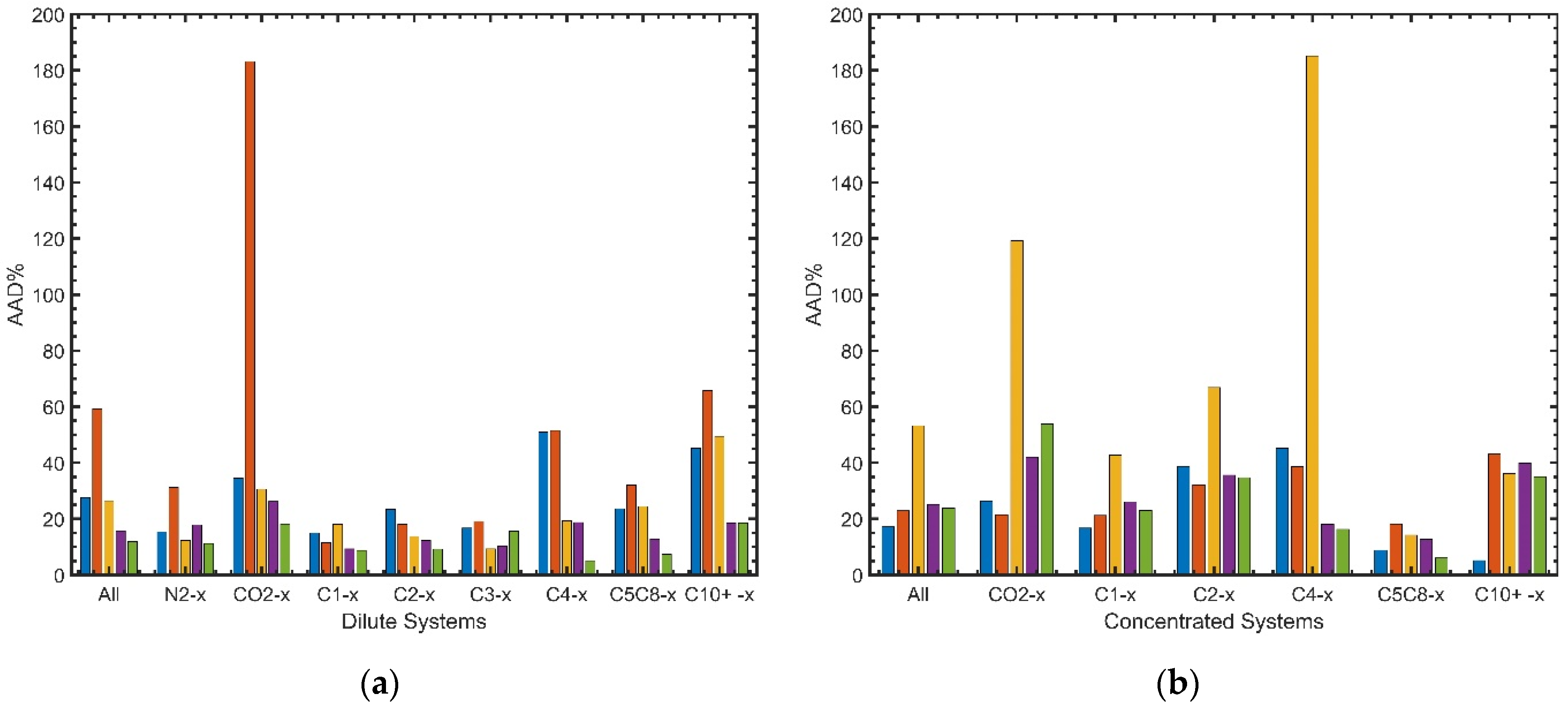
5.2. Overall Results from the Base Case Calculation

The binary diffusion coefficients were calculated using five different correlations, with the base case options selected for various properties. We first include all the data covering the whole concentration range and then distinguish different concentration ranges. The C₁-C₁₀ data from [79] were not included in the comparison in Section 5. Some of the data were close to the mixture critical point and exhibited unusual features, such as an increasing diffusion coefficient with pressure. In addition, the calculated diffusion coefficients were sensitive to the modeling of equilibrium, density, and viscosity close to the critical point. Inclusion of the data can change the average deviations for different correlations dramatically. In the supplementary materials, we have included some figures where the inclusion of the data can provided noticeable influence.

• Whole concentration range

Table S1 (supplementary materials) provides the detailed absolute average deviation (AAD%) for different systems and correlations. Figure 10 shows the AAD% and maximum absolute deviations (MAD%) for all the systems and different groups, such as N₂-X, CO₂-X, C₁-X, etc. These groups were characterized by the first components in their names and correspond to the columns for these first components in Table 1. The data in such a group represent the diffusion coefficients of the first component in the liquid phase mixture consisting of the first and second components.

From Table S1, it is obvious that most of the AAD% were in the range of 10–100%. The deviations were much larger than the deviations in typical density modeling for similar systems [142,143]. The larger deviations can be attributed to the quality of the experimental data and difficulty of accurate measurement of diffusion coefficients, as well as the challenge in modeling diffusion coefficients.

In Figure 10a, the AAD% for all the systems and different groups were within or around 100%, except for the abnormally large deviation by RW for CO₂-X and large deviation by LDF for C₄-X. Overall, HM provided the lowest deviation (21%), followed by WC (25%). For different groups, HM provided the lowest deviations, except for C₃-X, where LDF provided the lowest deviation. Actually, for the AAD% in Figure 10a, HM and WC were often similar, whereas the other three correlations were generally comparable. Figure 10a also shows that the differences between different correlations were limited for the lighter components (N₂-X to C₃-X), mostly within 10%. For C₄-X to C₁₀₊-X, ES, RW, and LDF tended to provide larger deviations. Among ES, RW, and LDF, ES seemed to provide a more stable performance, in contrast to the high deviations for C₅C₈-X (C₅C₈ stands from C₅ to C₈) for and C₁₀₊-X by RW and C₁-X and C₄-X by LDF.

The MAD% in Figure 10b is another important performance indicator for these correlations because it is desirable to have a smaller maximum deviation when modeling a certain type of systems. If we include all the data, ES provided the smallest MAD%, followed by LDF. WC and HM were similar, providing larger MAD%. RW provided the worst MAD%, due to the problem for CO₂-X. However, if we look at different groups, WC and HM actually provided the smallest MAD% for groups heavier than C₃-X. For CO₂-X, WC and HM provided much higher MAD% than ES and LDF. The high maximum deviations happen at high solute mole fractions, somewhat suggesting the limitation of WC and HM in describing the concentration dependence, as compared to ES and LDF. ES provided the lowest MAD% for both C₁-X and CO₂-X. LDF provided a similar low MAD% for CO₂-X, but it provided the highest MAD% for C₁-X, C₂-X, and C₄-X. ES also provided high MAD% for systems heavier than C₂-X.

CO₂-X was a problematic system that provided high MAD% for all correlations, especially RW. An abnormally large deviation appeared with RW for CO₂+C₁₆. For RW, its MAD% for CO₂-X was exceptionally high. The large deviation for RW was caused by two inherent problems in the correlation. First, the sign of the c parameter in Equation (14) directly determined the pressure dependence of the diffusion coefficient. For heavy components with large acentric factors (e.g., 0.72 for C₁₆), the c parameter changed its sign at a moderate pressure. This provides the wrong pressure dependence, and the deviation became pronounced when the pressure range was large. The wrong pressure dependence also occurs with other heavy systems. It was just the large pressure range of CO₂-C₁₆ that resulted in more obvious deviations. Second, the CO₂-C₁₆ system had some recent data measured up to 690 bar. For a positive c caused by the large acentric factor, a very high reduced pressure can further change the sign of the exponent $(\mathrm{b}+\mathrm{c}{\mathrm{P}}_{\mathrm{r}})$ in Equation (14) from negative to positive, thus causing a wrong dependence on viscosity. Obviously, these problems at high acentric factors and high reduced pressures were not fully considered in the development of the RW correlation.

In summary, if all the binary data were included, WC and HM seemed to provide smaller AAD% and MAD% for relatively heavy components (C₄₊). For lighter components N₂, C₁, C₂, and C₃, the AAD% for these correlations were similar, except for the fact that RW for N₂ and LDF for C₁ were poorer than the others. LDF also provided higher AAD for C₄-X.

• Different concentration ranges

Correlations such as WC and HM were essentially developed for dilute solutions. It is, therefore, meaningful to evaluate all the five correlations at different concentration ranges. We chose an arbitrary small mole fraction of 0.15 as the threshold to distinguish between the “dilute” mixtures and “concentrated” ones. This means that, for a mixture of A-B, the ranges x_A < 0.15 and x_B < 0.15 were considered dilute, with the remaining range considered concentrated. There were 698 and 464 points, respectively, in these two ranges. It should be noted that the data for N₂-X and C₃-X were only in the dilute range. Figure 11 summarizes the results for these two ranges.

For the dilute solutions (Figure 11a), HM was more accurate. It provided the lowest deviations for all the groups except C₃-X, and its performance for C₃-X was also comparable to the others. For heavier systems, HM tended to provide lower deviations. WC was similar to HM, but not as good. ES and LDF were similar, with their total AADs around 27%. RW seemed to be inferior to the others in the dilute range, providing the highest deviations for all the groups, except C₁-X and C₂-X.

For the concentrated solutions (Figure 11b), ES provided the lowest overall deviation, followed by RW. RW provided the smallest deviation for CO₂-X and C₂-X, but the highest deviation for C₅C₈-X and C₁₀₊-X. RW seemed to be the best for the light concentrated solutions. WC and HM were similar to RW, but slightly worse for many groups. LDF was obviously inferior to the other correlations, providing the highest deviations for CO₂-X, C₁-X, C₂-X, and C₄-X.

5.3. Sensitivity to the Property Models

The selection of the models in the base case calculation was a bit arbitrary. Even though we tried to select the most accurate models, these diffusion coefficient correlations were not necessarily developed with the most accurate ones. For example, LDF was developed using PR-VT for density and composition derivatives, the corresponding states (CS) viscosity model of Pedersen et al. [206,214] for viscosity, and the Fuller method for the low-pressure density-viscosity product. Hence, it is useful to study the sensitivity of the calculation to these property models. Among the properties listed in Table 5, density affects ES, RW, and LDF, viscosity affects all the correlations except for ES, and the last two properties (the composition derivatives and low-pressure density-diffusivity product) affect LDF only. Although ES and RW also use the low-pressure density-diffusivity product, it makes little sense to switch their default Chapman–Enskog model to the Fuller model.

• Influence of the density models

In the comparison of the density models, it should be noted that not all the systems can be described by GERG. It can be applied to only 32 “GERG systems” that do not contain components heavier than C₁₀. Our sensitivity analysis needs to differentiate between the results for these GERG systems and those for all systems. It should also be noted that we kept all the other options the same, as in the base case, when varying the density model.

Figure 12 shows the influence of density models on the AAD% from three correlations (WC and HM do not use density as input). For the GERG systems (Figure 12a), we can see that only ES was significantly affected if SRK was used. The observation has several implications. First, these diffusion coefficient models have certain tolerance to the deviation in density. Although GERG was the most accurate and PR-VT, SRK-VT, and SAFT were supposed to be more accurate than PR, these differences seem to have little influence on the calculated diffusion coefficients. Second, it shows that SRK without VT provides a density that is too inaccurate for some systems, thus increasing the deviation dramatically for ES. Finally, the results for RW and LDF were not so affected, even though SRK was used, thus showing that these two models were not so sensitive to density. Indeed, the two models assumed an exponential dependence of diffusion coefficient on viscosity, and the direct density influence was only through the density-diffusivity product. In principle, density calculation can also influence viscosity in some models, e.g., LBC. However, our sensitivity analysis here only considered the direct influence from a single factor.

If we include all systems (Figure 12b), the deviations become higher for ES and RW and lower for LDF after the inclusion of the heavier systems. The differences in the density from PR-VT, SRK-VT, and SAFT have little influence on the estimated diffusion coefficients. However, PR, apart from SRK, also increases the deviation from ES obviously. For heavy components, PR without VT provided poorer density description. This shows, again, that ES is more sensitive to density, whereas the density dependence is weaker in RW and LDF.

• Influence of the viscosity models

Figure 13 shows the AAD% for RW, LDF, WC, and HM with four viscosity models FT-SRK, FT-PR, LBC-PR, and LBC-PRVT. ES was excluded, since it does not depend on viscosity. Among these viscosity models, FT-SRK, FT-PR, and LBC-PRVT have comparable accuracy in viscosity estimation for common mixtures. LBC-PR provided the most inaccurate viscosity, due to the relatively inaccurate density from PR without VT. Figure 13 presents the AAD% for all systems, as well as some selected groups. FT-PR and FT-SRK provided almost identical results. LBC-PRVT, due to its slightly inferior viscosity, especially for heavier systems, provided larger deviations than FT-PR and FT-SRK, with CO₂-X calculated by RW being an exception for the issue explained in Section 5.2. The inaccurate viscosity with LBC-PR should, in principle, lead to larger deviations in the estimated diffusion coefficients. This is the case for LBC-PR with WC or HM. However, it is not the case for RW and LDF for all systems in Figure 13a. There are several reasons for this, including the abnormal behavior in CO₂-X, a potential error cancellation in some heavy systems (Figure 13d), and the relative insensitivity to viscosity for RW and LDF. Actually, the deviations for RW and LDF varied to a much smaller extent than those for WC and HM. LBC-PRVT is the default model used in the development of RW. We can find some groups supporting the use of LBC-PRVT as the best option for RW, as well as some counter examples. The differences were generally not large. Nevertheless, considering the obvious benefits of using FT-SRK or FT-PR for WC or HM, using a more accurate viscosity model seems to be the most sensible choice.

• Options for LDF

A unique feature of LDF is that it requires the composition derivatives of fugacity coefficients from an EoS. PR was used in the base case calculation, but other EoS (GERG, SRK, and SAFT) could also be used. Figure 14 presents a comparison between these EoS for the GERG systems, as well as for all systems. The differences between these models were generally small for both types of systems. Actually, SRK and PR provided almost identical results, and SAFT differed from these two EoS very slightly. GERG seemed to be more different and actually increased the deviation.

The original LDF correlation uses the Fuller model, instead, for the low-pressure density-diffusivity product, and the corresponding states (CS) viscosity model of Pedersen et al. [206] for viscosity. In our base case calculation, the Chapman–Enskog model and FT-PR were used instead, and Chapman–Enskog was also the default model in ES and RW. It would be interesting to know whether the options in the base case model deteriorate the LDF performance. Here, we use another corresponding states viscosity model CS2 [214] as a substitute for CS. CS2, developed a few years after CS, is believed to deliver similar viscosity results. As shown in Figure 15, if we kept FT-PR for viscosity and change Chapman–Enskog to Fuller, the deviation increased for most systems, especially C₅₊. This seems to suggest that Fuller may not be a better option than Chapman–Enskog here. We can further include the variation of the viscosity model. However, it turns out that using the options close to those suggested in the original paper (Fuller and CS2) did not necessarily provide the lowest deviation. The options used in our base case (Chapman–Enskog and FT-PR) actually provided the smallest deviation for all systems, although the ranking varied with the group. There was no clear indication that the original options provided a smaller deviation. It shows that our selection of various property models in the base case was reasonable.

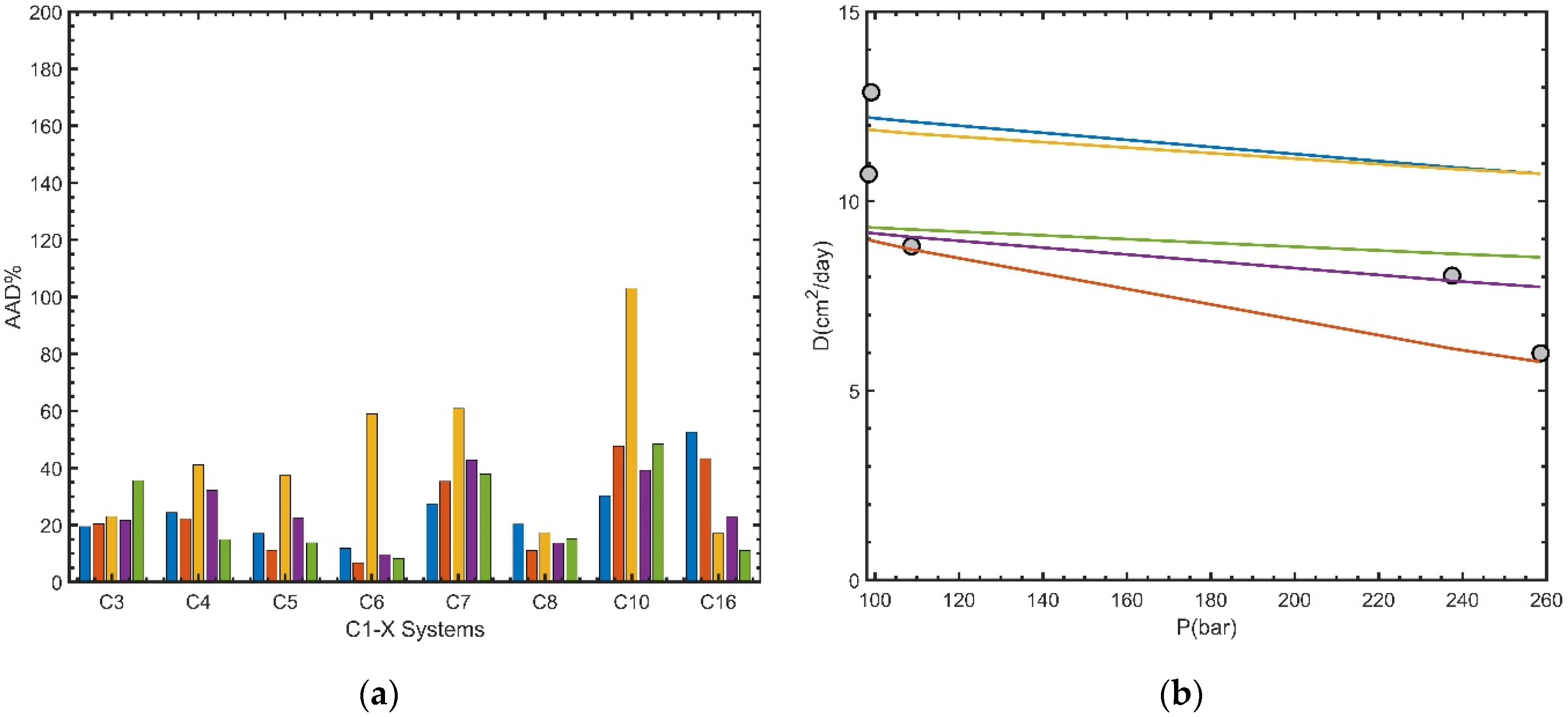
5.4. Results for Selected Groups

Among the binary groups, C₁-X and CO₂-X are typical examples for diffusion of light gas components in liquid. N₂-X is another example of this type of diffusion, but there were only two such systems (N₂-C₈ and N₂-C₁₀) in our database. For reservoir processes, C₁ and CO₂ are particularly important because C₁ is the major component in the gas phase and CO₂ can also present in a large amount; additionally, both are the most common components in gas injection.

Figure 16a presents the results for eight C₁-X systems. HM provided the best overall performance, although its deviation for C₃-X was the highest. RW was the second best, providing the lowest deviations in C₁-C₅, C₁-C₆, and C₁-C₈. ES provided the lowest deviation in C₁-C₃, C₁-C₇, and C₁-C₁₀, with the highest deviation for heavier systems C₁-C₁₀ and C₁-C₁₆. LDF, despite its theoretical basis, was inferior to all the other correlations and had the highest deviations in C₁-C₄, C₁-C₅, C₁-C₆, C₁-C₇, and C₁-C₁₀. Figure 16b illustrates a typical result at one selected temperature. The few data points were scattered, but a decreasing trend with pressure can be observed. RW provided the best description here; in particular, it captured the high-pressure point better, which can also be observed at other temperatures.

Figure 17a summarized the deviations in 12 CO₂-X systems. RW did not perform well here, due not only to its abnormal behavior for C₁₆ but also the large deviations, in general, for other systems. LDF seemed to be second worst, providing highest deviations in CO₂-C₅, CO₂-C₈, CO₂-C₁₀, and CO₂-C₁₄. HM was the best correlation here, despite its high deviation for CO₂-C₅, CO₂-C₇, and CO₂-C₁₄. WC followed the trend of HM but generally provided an inferior performance. ES was similar to WC, in terms of the overall AAD, while WC was better for heavier systems such as C₂₀₊. Figure 17b presents the result for CO₂-C₁₆ at 348 K. HM provided perfect estimates for the diffusion coefficients at this temperature, as well as at other temperatures that were not shown here. ES also provided good description here, but over- or under-predicted at other temperatures. LDF and WC under-predicted the diffusion coefficients. RW predicted a wrong trend with pressure.

Figure 18 presents the results for two selected groups, C₂-X and C₁₂-X, which somewhat represent the performance for the light component diffusion and that of heavy component diffusion. For C₂-X, HM provided the best overall performance, and it tended to provide smaller deviations for heavier components. WC resembleed HM, but its performance was not as good. RW provided a relatively stable performance, as compared to LDF and ES. For C₁₂-X, HM and WC were clearly the best, with HM being slightly better. The other three provided comparable results, with ES being slightly better in this case.

6. Results for Oil Mixtures

It is more difficult to evaluate the diffusion coefficient correlations using the oil data because of the incomplete information for oil composition and oil properties. To use ES, RW, and LF, a complete compositional fluid description is needed, and the fluid model should, in principle, be tuned against the PVT data at the experimental conditions. Unfortunately, most oils in the databank did not have detailed compositional information; even for those with a compositional fluid model in the original literature, it was not always clear whether the model was applicable to viscosity calculation, as well. WC and HM do not require compositional information. Both require the viscosity data at the experimental condition. For WC, we also needed the oil molecular weight, which was not always provided. Therefore, we could only evaluate several correlations here, depending on the availability of the oil composition and other properties. We first presented the results for HM, which can be applied to most oils, even those without detailed composition for most oils. Then, we presented the comparison of several correlations for oils with sufficiently detailed composition information. However, LDF was not included here, since it requires a sophisticated transformation involving composition derivatives.

Table 6. AAD% in oil diffusion coefficients calculated by the HM correlation.

Type	Systems	Np	AAD%
Refined oil products	CO2 + kerosine [119]	1	37.3
	CO2 + white oil [197]	2	60.8
	C1 + white oil [191]	5	25.0
	C2 + white oil [193]	4	55.6
	C3 + kerosene [194]	19	60.3
	C3 + spray oil [194]	12	31.1
Average			45.0
Ordinary crude oil	CO2-crude oil [119,169,196,198]	17	600.0
Heavy oil and bitumen	N2 [146]	4	70.2
	CO2 [82,146,151,163,165,170,171,173,176,177,178,183,184,186,188]	31	89.9
	C1 [82,146,165,170,171,172,173,174]	20	90.5
	C2 [146,172]	7	96.1
	C3 [161,164,171,172,177,178]	15	94.6
	C4 [176,178]	2	99.8
	C5 [158,159,160,179]	48	99.1
	C6 [179]	1	100.0
	C7 [179]	8	99.9
Average			93.3
Total		196	106.9

summarizes the HM results for oil systems that did not have detailed composition information but did have experimental viscosity data. Most of the oil systems belong to heavy oils. There are just a few ordinary crude oils and several oil products. All these oil systems were de-gassed oil. The diffusion coefficients were for different gases and solvents, with CO₂ and C₁ being the most common ones. HM provided an average AAD% of 45% for the relatively light oil products. For the ordinary crude oil, it over-predicted the diffusion coefficient by six times. For heavy oil and bitumen, the deviations were around 90–100%. Although the deviations seemed to be acceptable, a more detailed look at these deviations shows that HM systematically under-predicts the diffusion coefficients by one to two orders of magnitude, and the predictions for the heavy oils were actually the worst among the three types of oils. Overall, we can expect reasonable accuracy from HM for relatively light oils; the predictions became more uncertain for heavier oils, which is not surprising, considering HM was developed using paraffins with viscosities orders of magnitude smaller than those of heavy oils and bitumen.

Table 7. Deviations (%) in oil diffusion coefficients calculated by ES, RW, WC and HM.

Systems	ES	RW	WC	HM	Viscosity
Light oils
C1 in light oil [189]	−83.5	119.1	33.1	135.7	LBC
CO2 in live oil [154]	−0.5	769.8	1065.7	1623.1	LBC
CO2 in STO [154]	−57.7	−38.4	−73.7	−28.9	LBC
C1 in live oil [152]	−56.0	−2.7	−50.1	−29.4	LBC
Heavy oils
CO2 in heavy oil [176]	2709.5	−72.0	−98.2	−67.9	Paper
CO2 in heavy oil [176]	1077.2	−88.2	−99.3	−86.7	Paper
CO2 in heavy oil [176]	2794.4	−96.9	−99.9	−94.1	Paper
CO2 in heavy oil [185]	2677.7	−93.8	−99.9	−92.0	Paper
CO2 in heavy oil [185]	1145.7	−93.4	−99.7	−91.1	Paper
CO2 in heavy oil [185]	516.8	−94.0	−99.5	−91.5	Paper
AAD
Light oils	49.4	232.5	305.7	454.3
Heavy oils	1820.2	89.7	99.4	87.2
All	1111.9	146.8	181.9	234.0

presents the results for a limited number of oils that have sufficient compositional information for an EoS modeling for ES and RW. We can also extract the viscosity data from some of these sources and directly use them in RW, WC, and HM. However, the experimental viscosities were often missing, and we needed to use the LBC viscosity model to estimate the viscosity together with the EoS model recommended in the original paper. All these diffusion coefficients were measured by CVD, where the composition of the oil phase varied with time. In the comparison, we always used the original oil composition or the oil composition in the beginning of CVD for estimating the diffusion coefficients. For the case [152], the original paper does not provide effective diffusion coefficients, we therefore used the effective diffusion coefficients fitted in [153]. The measurement by Ghasemi et al. [154] is actually in a porous rock. We calculated the corresponding bulk phase diffusion coefficients using the tortuosity provided in their paper. These two cases [152,154] are included in Table 7, although they are not included in Table 4.

In Table 7, the first four systems are relatively light oils including several live oils, the last six systems are heavy oils. The performances of the correlations are different for the two types of oils. For light oils, ES tends to under-predict the coefficients, and the other three (RW, WC, and HM) provided significant over-predictions in several cases. The AAD% for ES was smaller than those for the other three correlations. None of the correlations is consistently better than the others. For [154], the coefficient reported in the original study was obtained using ES, thus giving a good agreement here. For heavy oil systems, RW, WC, and HM tend to under-predict the diffusion coefficients, often by 1–2 orders of magnitude, and ES tends to over-predict the coefficients. According to the study in Section 5.3, ES is sensitive to density whereas RW, WC, and HM are sensitive to viscosity. It should be noted that the viscosity for the light oils were calculated by LBC, and it was not always clear whether the EoS reported in the original literature is tuned for experimental viscosity. Therefore, this uncertainty in viscosity may contribute to larger deviations for RW, WC, and HM. However, for heavy oils, where the viscosities are directly from the literature, the three correlations provided significant and systematic under-predictions, which should be attributed to some inherent problems in the correlations. Finally, we should bear in mind that the above findings are summarized based on a limited number of cases.

7. Conclusions

Diffusion coefficients in well-defined mixtures or oils are fundamental to understanding diffusion in various reservoir processes, such as gas injection in tight formation and fractured reservoirs. In this study, we have provided an extensive collection of the diffusion coefficients of reservoir fluids-related systems. Two databases, one for the binary mixtures and another for multicomponent oil mixtures, have been established. Using the database, five commonly-used diffusion coefficient models have been evaluated. The main conclusions of this study are:

• The binary diffusion coefficients database has over 1600 data points, with around 1300 liquid-phase diffusion data points. These liquid-phase diffusion coefficients are influenced by factors including the component type, composition, temperature, and pressure. In the database, the liquid-phase diffusion coefficient for methane can reach 50 cm²/day, and the coefficient for CO₂ can reach 200 cm²/day, while the minimum values are around 0.5–1 cm²/day for C₁ and CO₂. In general, the diffusion coefficient increases with increasing temperature, decreasing pressure, and increasing concentration of the light solute. There were over 400 data points in the oil diffusion database, with over half of them for heavy oils. The diffusion coefficients for C₁/CO₂/N₂-heavy oil were mostly in the range of 0.01–50 cm²/day. Those for C₁/CO₂/N₂-non-heavy oils were mostly in the range of 0.01–150 cm²/day.
• There was a lack of data in both the binary mixtures and oil systems. The number of available binary diffusion data collected here is just a small fraction (>20× smaller) of the available density data for the similar systems. Anyway, the quality of the diffusion coefficients is an issue, in terms of accuracy and completeness—many diffusion data did not have the corresponding composition. The oil diffusion coefficients were even more scarce, and their quality was more questionable. The reported oil diffusion coefficients may differ in orders of magnitude. Only a limited number of studies report oil compositions, and the studies on live oils were rare.
• The scarcity of diffusion data is in a noteworthy contrast to the significance of diffusion in various reservoir processes. It underscores the need for more experimental measurement. The data for binary mixtures, especially for gas-liquid mixtures at high pressures, are crucial for developing the fundamental diffusion models. For oil mixtures, it is worthwhile to include diffusion measurement as part of the PVT study, especially for gas injection. Publishing more oil diffusion data in the open literature should also be encouraged.
• Among the five correlations studied here, HM and WC have the same theoretical basis (the Stokes–Einstein equation); both ES and RW use an empirical correction to calculate the real fluid diffusion coefficient from the dilute gas one, and LDF is the only one using the MS framework. In comparison with large databases, no single correlation showed a consistent and dominant superiority over the others. Nevertheless, it is possible to find some general trends or identify some more suitable models for specific regions or systems. These details, presented in Section 5 and Section 6, are useful when selecting a correlation for specific applications.
• For binary mixtures, HM provides the lowest deviations, and it is particularly good for diluted solutions and heavier systems. WC provides a similar, but somewhat inferior, performance. However, it should be noted that both HM and WC had a consistency issue because both were originally developed for the diffusion of solute in solvent, and the definitions of solute and solvent are ambiguous at high concentrations. In concentrated composition range, ES seems to be the best choice, and RW is also a good choice. It should be noted that RW has a problem for systems containing a heavy component with a large acentric factor at high-reduced pressures, thus causing large deviations and abnormal pressure dependence for systems such as CO₂-C₁₆. RW will become more attractive if this problem is fixed. LDF, despite its strong theoretical basis, did not really show any obvious advantage over the other correlations. It provides good results in the dilute range. Its results at any non-zero concentrations were essentially from the Vignes mixing rule. The correlation tended to provide large deviations for gas-liquid systems such as C₁-C₁₀. Although the comparison of the five correlations was based on an extensive binary database, it should be noted that the conclusion regarding the correlation performance depended much on the data selected in the comparison. The recommendation for the best model depends on the system and range of temperature, pressure, and composition. The comparison here was more to reveal the strengths and limitations of these correlations.
• The results for diffusion coefficients also depend on the models selected for density, viscosity, and other properties. A sensitivity study using the binary database has shown that our selection in the base case is reasonable. We can always select the most accurate models for these properties, even though the models used in developing the original correlations may be different. Furthermore, if the modeled density and viscosity are beyond a certain accuracy, the influence of the models become unimportant. For example, GERG, PR-VT, SRK-VT, and SAFT-VT generally provided comparable results, and FT-PR, FT-SRK, and LBC-PRVT provided comparable results. The sensitivity analysis also reveals different degrees of sensitivity of these correlations to the property models. HM and WC were sensitive to viscosity, and ES was sensitive to density. RW and LDF had weak dependence on viscosity.
• For oil systems, HM was the easiest to use, since it requires the smallest set of input parameters. Many of the collected oils could only be tested with HM. HM seemed to provide reasonable results for ordinary oils and light oil products but had a tendency to under-estimate the gas diffusion in heavy oils. Only a limited number (10) of oil systems have sufficient composition information that allow for the use of an EoS model. Among the four correlations (ES, RW, HM, and WC) tested, ES tended to under-predict the diffusion coefficients for light oils but over-predict the results for heavy oils, whereas RW, HM, and WC seemed to have the opposite tendency. For heavy oils, RW, HM, and WC tended to under-estimate the diffusion coefficients by one to two orders of magnitude. The findings based on the small set of data should be used with caution.

As a final remark, diffusion coefficients in reservoir fluids involve a wide range of topics, and we only focused on the bulk liquid-phase diffusion for both binaries and oils here. There seemed to be less effort in measuring binary diffusion data in recent years, although we do not possess systematic and accurate data for these binaries. This might be attributed to the two following reasons. First, other popular systems with high scientific and technological value have diverted researchers’ interest. For example, the measurement of CO₂ diffusion in water or brine becomes essential for underground CO₂ storage. Second, researchers often need to address the diffusion problem in complex oil mixtures more directly, instead of accumulating more knowledge about the relevant binaries first. In recent years, gas/solvent diffusion in heavy oil, diffusion in tight formation, diffusion in porous media, and diffusion in live oils were some active research areas. In addition, there has been active research to improve the data processing for diffusion measurement in oil mixtures. In the long term, for a better description of the diffusion process in a reservoir, it is important to study both relevant binaries and various reservoir fluids.

References

1. Poling, B.E.; Prausnitz, J.M.; O’connell, J.P. The Properties of Gases and Liquids; McGraw-Hill Education: New York, NY, USA, 2001. [Google Scholar]
2. Medvedev, O. Diffusion Coefficients in Multicomponent Mixtures. Ph.D. Thesis, Technical University of Denmark, Kgs. Lyngby, Denmark, 2005. [Google Scholar]
3. Oelkers, E.H.; Helgeson, H.C. Calculation of the Thermodynamic and Transport Properties of Aqueous Species at High Pressures and Temperatures: Aqueous Tracer Diffusion Coefficients of Ions to 1000 °C and 5 Kb. Geochim. Cosmochim. Acta 1988, 52, 63–85. [Google Scholar] [CrossRef]
4. Desai, T.A.; Hansford, D.J.; Kulinsky, L.; Nashat, A.H.; Rasi, G.; Tu, J.; Wang, Y.; Zhang, M.; Ferrari, M. Nanopore Technology for Biomedical Applications. Biomed. Microdevices 1999, 2, 11–40. [Google Scholar] [CrossRef]
5. Chordia, M. Diffusion in Naturally Fractured Reservoirs—A Review. In Proceedings of the SPE Asia Pacific Oil & Gas Conference and Exhibition, Brisbane, QLD, Australia, 18 October 2010. [Google Scholar]
6. Jia, B.; Tsau, J.-S.; Barati, R. A Review of the Current Progress of CO2 Injection EOR and Carbon Storage in Shale Oil Reservoirs. Fuel 2019, 236, 404–427. [Google Scholar] [CrossRef]
7. Hunt, E.B., Jr.; Berry, V.J., Jr. Evolution of Gas from Liquids Flowing through Porous Media. AIChE J. 1956, 2, 560–567. [Google Scholar] [CrossRef]
8. Li, X.; Yortsos, Y. Theory of Multiple Bubble Growth in Porous Media by Solute Diffusion. Chem. Eng. Sci. 1995, 50, 1247–1271. [Google Scholar] [CrossRef]
9. Campbell, B.T.; Orr, F.M. Flow Visualization for CO2/Crude-Oil Displacements. SPE J. 1985, 25, 665–678. [Google Scholar] [CrossRef]
10. Grogan, A.; Pinczewski, W. The Role of Molecular Diffusion Processes in Tertiary CO2 Flooding. J. Pet. Technol. 1987, 39, 591–602. [Google Scholar] [CrossRef]
11. Da Silva, F.V.; Belery, P. Molecular Diffusion in Naturally Fractured Reservoirs: A Decisive Recovery Mechanism. In Proceedings of the 6th Annual Technical Conference and Exhibition of the Society of Petroleum Engineers, San Antonio, TX, USA, 8 October 1989. [Google Scholar]
12. Ghasemi, M.; Suicmez, V. Upscaling of CO2 Injection in a Fractured Oil Reservoir. J. Nat. Gas Sci. Eng. 2019, 63, 70–84. [Google Scholar] [CrossRef]
13. Trivedi, J.; Babadagli, T. Experimental and Numerical Modeling of the Mass Transfer between Rock Matrix and Fracture. Chem. Eng. J. 2009, 146, 194–204. [Google Scholar] [CrossRef]
14. Alavian, S.A.; Whitson, C.H. Modeling CO2 Injection Including Diffusion in a Fractured-Chalk Experiment. In Proceedings of the SPE Annual Technical Conference and Exhibition, Florence, Italy, 19 September 2010. [Google Scholar]
15. Darvish, G.R.; Lindeberg, E.G.; Holt, T.; Utne, S.A.; Kleppe, J. Reservoir Conditions Laboratory Experiments of CO2 Injection into Fractured Cores. In Proceedings of the SPE Europec/EAGE Annual Conference and Exhibition, Vienna, Austria, 12 June 2006. [Google Scholar]
16. Hoteit, H.; Firoozabadi, A. Numerical Modeling of Diffusion in Fractured Media for Gas-Injection and-Recycling Schemes. SPE J. 2009, 14, 323–337. [Google Scholar] [CrossRef]
17. Alavian, S.A.; Whitson, C.H. Scale Dependence of Diffusion in Naturally Fractured Reservoirs for CO2 Injection. In Proceedings of the SPE Improved Oil Recovery Symposium, Tulsa, OK, USA, 24 April 2010. [Google Scholar]
18. Yanze, Y.; Clemens, T. The Role of Diffusion for Nonequilibrium Gas Injection into a Fractured Reservoir. SPE Res. Eval. Eng. 2012, 15, 60–71. [Google Scholar] [CrossRef]
19. Burrows, L.C.; Haeri, F.; Cvetic, P.; Sanguinito, S.; Shi, F.; Tapriyal, D.; Goodman, A.; Enick, R.M. A Literature Review of CO2, Natural Gas, and Water-Based Fluids for Enhanced Oil Recovery in Unconventional Reservoirs. Energy Fuels 2020, 34, 5331–5380. [Google Scholar] [CrossRef]
20. Hawthorne, S.B.; Gorecki, C.D.; Sorensen, J.A.; Steadman, E.N.; Harju, J.A.; Melzer, S. Hydrocarbon Mobilization Mechanisms from Upper, Middle, and Lower Bakken Reservoir Rocks Exposed to CO2. In Proceedings of the SPE Unconventional Resources Conference-Canada, Calgary, AB, Canada, 5 November 2013. [Google Scholar]
21. Yu, W.; Lashgari, H.R.; Wu, K.; Sepehrnoori, K. CO2 Injection for Enhanced Oil Recovery in Bakken Tight Oil Reservoirs. Fuel 2015, 159, 354–363. [Google Scholar] [CrossRef]
22. Wan, T.; Sheng, J. Compositional Modelling of the Diffusion Effect on EOR Process in Fractured Shale-Oil Reservoirs by Gasflooding. J. Can. Pet. Technol. 2015, 54, 107–115. [Google Scholar] [CrossRef]
23. Jin, L.; Hawthorne, S.; Sorensen, J.; Kurz, B.; Pekot, L.; Smith, S.; Bosshart, N.; Azenkeng, A.; Gorecki, C.; Harju, J. A Systematic Investigation of Gas-Based Improved Oil Recovery Technologies for the Bakken Tight Oil Formation. In Proceedings of the Unconventional Resources Technology Conference, San Antonio, TX, USA, 1 August 2016. [Google Scholar]
24. Alharthy, N.; Teklu, T.; Kazemi, H.; Graves, R.; Hawthorne, S.; Braunberger, J.; Kurtoglu, B. Enhanced Oil Recovery in Liquid–Rich Shale Reservoirs: Laboratory to Field. SPE Res. Eval. Eng. 2018, 21, 137–159. [Google Scholar] [CrossRef]
25. Das, S.K. Vapex: An Efficient Process for the Recovery of Heavy Oil and Bitumen. SPE J. 1998, 3, 232–237. [Google Scholar] [CrossRef]
26. Jiang, Q.; Butler, R.M. Selection of Well Configurations in Vapex Process. In Proceedings of the SPE International Conference on Horizontal Well Technology, Calgary, AB, Canada, 18 November 1996. [Google Scholar]
27. Butler, R.; Jiang, Q. Improved Recovery of Heavy Oil by VAPEX with Widely Spaced Horizontal Injectors and Producers. J. Can. Pet. Technol. 2000, 39, PETSOC-00-01-04. [Google Scholar] [CrossRef]
28. Cussler, E.L. Diffusion: Mass Transfer in Fluid Systems; Cambridge University Press: Cambridge, UK, 2009. [Google Scholar]
29. Leahy-Dios, A.; Firoozabadi, A. Unified Model for Nonideal Multicomponent Molecular Diffusion Coefficients. AIChE J. 2007, 53, 2932–2939. [Google Scholar] [CrossRef]
30. Fick, A.E. Ueber Diffusion. Ann. Phys. 1855, 170, 59–86. [Google Scholar] [CrossRef]
31. Maxwell, J.C., IV. On the Dynamical Theory of Gases. Philos. Trans. R. Soc. 1867, 157, 49–88. [Google Scholar] [CrossRef]
32. Onsager, L. Theories and Problems of Liquid Diffusion. Ann. N. Y. Acad. Sci. 1945, 46, 241–265. [Google Scholar] [CrossRef] [PubMed]
33. Taylor, R.; Krishna, R. Multicomponent Mass Transfer; John Wiley & Sons: New York, NY, USA, 1993. [Google Scholar]
34. Marrero, T.R.; Mason, E.A. Gaseous Diffusion Coefficients. J. Phys. Chem. Ref. Data 1972, 1, 3–118. [Google Scholar] [CrossRef]
35. Chapman, S.; Cowling, T.G. The Mathematical Theory of Non-Uniform Gases; Cambridge University Press: Cambridge, UK, 1991. [Google Scholar]
36. Einstein, A. Über Die von Der Molekularkinetischen Theorie Der Wärme Geforderte Bewegung von in Ruhenden Flüssigkeiten Suspendierten Teilchen. Ann. Phys. 1905, 322, 549–560. [Google Scholar] [CrossRef]
37. Neufeld, P.D.; Janzen, A.; Aziz, R. Empirical Equations to Calculate 16 of the Transport Collision Integrals Omega(l, s) for the Lennard-Jones (12–6) Potential. J. Chem. Phys. 1972, 57, 1100–1102. [Google Scholar] [CrossRef]
38. Dawson, R.; Khoury, F.; Kobayashi, R. Self-Diffusion Measurements in Methane by Pulsed Nuclear Magnetic Resonance. AIChE J. 1970, 16, 725–729. [Google Scholar] [CrossRef]
39. Sigmund, P.M. Prediction of Molecular Diffusion at Reservoir Conditions. Part 1-Measurement and Prediction of Binary Dense Gas Diffusion Coefficients. J. Can. Pet. Technol. 1976, 15, PETSOC-76-02-05. [Google Scholar] [CrossRef]
40. Arnold, J.H. Studies in Diffusion. II. A Kinetic Theory of Diffusion in Liquid Systems. J. Am. Chem. Soc. 1930, 52, 3937–3955. [Google Scholar] [CrossRef]
41. Aljeshi, Y.A.; Taib, M.B.M.; Trusler, J.M. Modelling the Diffusion Coefficients of Dilute Gaseous Solutes in Hydrocarbon Liquids. Int. J. Thermophys. 2021, 42, 140. [Google Scholar] [CrossRef]
42. Wilke, C.; Chang, P. Correlation of Diffusion Coefficients in Dilute Solutions. AIChE J. 1955, 1, 264–270. [Google Scholar] [CrossRef]
43. Hayduk, W.; Minhas, B. Correlations for Prediction of Molecular Diffusivities in Liquids. Can. J. Chem. Eng. 1982, 60, 295–299. [Google Scholar] [CrossRef]
44. Scheibel, E.G. Correspondence. Liquid Diffusivities. Viscosity of Gases. Ind. Eng. Chem. 1954, 46, 2007–2008. [Google Scholar] [CrossRef]
45. King, C.J.; Hsueh, L.; Mao, K.-W. Liquid Phase Diffusion of Non-Electrolytes at High Dilution. J. Chem. Eng. Data 1965, 10, 348–350. [Google Scholar] [CrossRef]
46. Rutten, P.W.M. Diffusion in Liquids. Ph.D. Thesis, Delft Univeristy, Delft, The Netherlands, 1992. [Google Scholar]
47. Riazi, M.R.; Whitson, C.H. Estimating Diffusion Coefficients of Dense Fluids. Ind. Eng. Chem. Res. 1993, 32, 3081–3088. [Google Scholar] [CrossRef]
48. Wesselingh, J.; Bollen, A. Multicomponent Diffusivities from the Free Volume Theory. Chem. Eng. Res. Des. 1997, 75, 590–602. [Google Scholar] [CrossRef]
49. Liu, H.; Silva, C.M.; Macedo, E.A. Generalised Free-Volume Theory for Transport Properties and New Trends about the Relationship between Free Volume and Equations of State. Fluid Phase Equilibria 2002, 202, 89–107. [Google Scholar] [CrossRef]
50. Bosma, J.; Wesselingh, J. Estimation of Diffusion Coefficients in Dilute Liquid Mixtures. Chem. Eng. Res. Des. 1999, 4, 325–328. [Google Scholar] [CrossRef]
51. Hsu, Y.-D.; Chen, Y.-P. Correlation of the Mutual Diffusion Coefficients of Binary Liquid Mixtures. Fluid Phase Equilibria 1998, 152, 149–168. [Google Scholar] [CrossRef]
52. Shapiro, A.A. Thermodynamic Theory of Diffusion and Thermodiffusion Coefficients in Multicomponent Mixtures. J. Non-Equilib. Thermodyn. 2020, 45, 343–372. [Google Scholar] [CrossRef]
53. Baghooee, H.; Shapiro, A. Unified Thermodynamic Modelling of Diffusion and Thermodiffusion Coefficients. Fluid Phase Equilibria 2022, 558, 113445. [Google Scholar] [CrossRef]
54. Darken, L.S. Diffusion, Mobility and Their Interrelation through Free Energy in Binary Metallic Systems. Trans. Aime 1948, 175, 184–201. [Google Scholar]
55. Vignes, A. Diffusion in Binary Solutions. Variation of Diffusion Coefficient with Composition. Ind. Eng. Chem. Fundamen. 1966, 5, 189–199. [Google Scholar] [CrossRef]
56. Himmelblau, D. Diffusion of Dissolved Gases in Liquids. Chem. Rev. 1964, 64, 527–550. [Google Scholar] [CrossRef]
57. Sigmund, P.M. Prediction of Molecular Diffusion at Reservoir Conditions. Part II-Estimating the Effects of Molecular Diffusion and Convective Mixing in Multicomponent Systems. J. Can. Pet. Technol. 1976, 15, 53–62. [Google Scholar] [CrossRef]
58. Berry, V.J., Jr.; Koeller, R. Diffusion in Compressed Binary Gaseous Systems. AIChE J. 1960, 6, 274–280. [Google Scholar] [CrossRef]
59. Gover, T.A. Diffusion of Gases: A Physical Chemistry Experiment. J. Chem. Educ. 1967, 44, 409. [Google Scholar] [CrossRef]
60. Reamer, H.; Sage, B. Diffusion Coefficients in Hydrocarbon Systems. Methane in the Liquid Phase of the Methane-Propane System. Ind. Eng. Chem. Chem. Eng. Data Ser. 1958, 3, 54–59. [Google Scholar] [CrossRef]
61. Woessner, D.; Snowden, B.S., Jr.; George, R.; Melrose, J. Dense Gas Diffusion Coefficients for the Methane-Propane System. Ind. Eng. Chem. Fundamen. 1969, 8, 779–786. [Google Scholar] [CrossRef]
62. Zangi, P.; Rausch, M.H.; Fröba, A.P. Binary Diffusion Coefficients for Gas Mixtures of Propane with Methane and Carbon Dioxide Measured in a Loschmidt Cell Combined with Holographic Interferometry. Int. J. Thermophys. 2019, 40, 18. [Google Scholar] [CrossRef]
63. Reamer, H.; Sage, B. Diffusion Coefficients in Hydrocarbon Systems. Methane-n-Butane-Methane in Liquid Phase. Ind. Eng. Chem. Chem. Eng. Data Ser. 1956, 1, 71–77. [Google Scholar] [CrossRef]
64. Christoffersen, K.R. High-Pressure Experiments with Application to Naturally Fractured Chalk Reserviors. Ph.D. Thesis, The Norwegian Institute of Technology University of Trondheim, Trondheim, Norway, 1992. [Google Scholar]
65. Riazi, M.R. A New Method for Experimental Measurement of Diffusion Coefficients in Reservoir Fluids. J. Pet. Sci. Eng. 1996, 14, 235–250. [Google Scholar] [CrossRef]
66. Imai, M.; Sumikawa, I.; Yamada, T.; Nakano, M. Reservoir Fluid Characterization for Tight Fractured Reservoirs: Effect of Diffusion. In Proceedings of the SPE Asia Pacific Oil and Gas Conference and Exhibition, Perth, Australia, 22 October 2012. [Google Scholar]
67. Reamer, H.; Duffy, C.; Sage, B. Diffusion Coefficients in Hydrocarbon Systems: Methane-n-Pentane-Methane in Liuqid Phase. Ind. Eng. Chem. 1956, 48, 282–284. [Google Scholar] [CrossRef]
68. Hill, E.; Lacey, W. Rate of Solution of Methane in Quiescent Liquid Hydrocarbons. II. Ind. Eng. Chem. 1934, 26, 1324–1327. [Google Scholar] [CrossRef]
69. Wilhelm, E.; Battino, R. Binary Gaseous Diffusion Coefficients. 1. Methane and Carbon Tetrafluroide with n-Hexane, n-Heptane, n-Octane, and 2,2,4-Trimethylpentane at One-Atmosphere Pressure at 10–70. Deg. J. Chem. Eng. Data 1972, 17, 187–189. [Google Scholar] [CrossRef]
70. Hayduk, W.; Buckley, W. Effect of Molecular Size and Shape on Diffusivity in Dilute Liquid Solutions. Chem. Eng. Sci. 1972, 27, 1997–2003. [Google Scholar] [CrossRef]
71. Kohn, J.P.; Romero, N. Molecular Diffusion Coefficients in Binary Gaseous Systems at One Atmosphere Pressure. N-Hexane-Methane and 3-Methylpentane-Methane Systems. J. Chem. Eng. Data 1965, 10, 125–127. [Google Scholar] [CrossRef]
72. Reamer, H.; Sage, B. Diffusion Coefficients in Hydrocarbon Systems: Methane in the Liquid Phase of the Methane–n-Heptane System. AIChE J. 1957, 3, 449–453. [Google Scholar] [CrossRef]
73. Taib, M.B.M.; Trusler, J.M. Diffusion Coefficients of Methane in Methylbenzene and Heptane at Temperatures between 323 K and 398 K at Pressures up to 65 MPa. Int. J. Thermophys. 2020, 41, 119. [Google Scholar] [CrossRef]
74. Colgate, S.; House, V.; Thieu, V.; Zachery, K.; Hornick, J.; Shalosky, J. High-Pressure Cylindrical Acoustic Resonance Diffusion Measurements of Methane in Liquid Hydrocarbons. Int. J. Thermophys. 1995, 16, 655–662. [Google Scholar] [CrossRef]
75. Killie, S.; Hafskjold, B.; Borgen, O.; Ratkje, S.K.; Hovde, E. High-Pressure Diffusion Measurements by Mach-Zehnder Interferometry. AIChE J. 1991, 37, 142–146. [Google Scholar] [CrossRef]
76. Erkey, C.; Akgerman, A. Translational-Rotational Coupling Parameters for Mutual Diffusion in N-Octane. AIChE J. 1989, 35, 443–448. [Google Scholar] [CrossRef]
77. Reamer, H.; Opfell, J.; Sage, B. Diffusion Coefficients in Hydrocarbon Systems. Methane-Decane-Methane in Liquid Phase. Ind. Eng. Chem. 1956, 48, 275–282. [Google Scholar] [CrossRef]
78. Dysthe, D.K.; Hafskjold, B.; Breer, J.; Cejka, D. Interferometric Technique for Measuring Interdiffusion at High Pressures. J. Phys. Chem. 1995, 99, 11230–11238. [Google Scholar] [CrossRef]
79. Dysthe, D.; Hafskjold, B. Inter-and Intradiffusion in Liquid Mixtures of Methane and n-Decane. Int. J. Thermophys. 1995, 16, 1213–1224. [Google Scholar] [CrossRef]
80. Jamialahmadi, M.; Emadi, M.; Müller-Steinhagen, H. Diffusion Coefficients of Methane in Liquid Hydrocarbons at High Pressure and Temperature. J. Pet. Sci. Eng. 2006, 53, 47–60. [Google Scholar] [CrossRef]
81. Pacheco-Roman, F.J.; Hejazi, S.H.; Maini, B.B. Estimation of Low-Temperature Mass-Transfer Properties of Methane and Carbon Dioxide in n-Decane, Hexadecane, and Bitumen Using the Pressure-Decay Technique. Energy Fuels 2016, 30, 5232–5239. [Google Scholar] [CrossRef]
82. Etminan, S.R.; Maini, B.B.; Chen, Z.; Hassanzadeh, H. Constant-Pressure Technique for Gas Diffusivity and Solubility Measurements in Heavy Oil and Bitumen. Energy Fuels 2010, 24, 533–549. [Google Scholar] [CrossRef]
83. Ratnakar, R.R.; Dindoruk, B. Measurement of Gas Diffusivity in Heavy Oils and Bitumens by Use of Pressure-Decay Test and Establishment of Minimum Time Criteria for Experiments. SPE J. 2015, 20, SPE-170931-PA. [Google Scholar] [CrossRef]
84. Erkey, C.; Akgerman, A. Translational Rotational Coupling Parameters for Mutual Diffusion in Normal Alkanes. AIChE J. 1989, 35, 1907–1911. [Google Scholar] [CrossRef]
85. Reamer, H.; Sage, B. Diffusion Coefficients in Hydrocarbon Systems. Ethane in the Liquid Phase of the Ethane-n-Pentane System. J. Chem. Eng. Data 1961, 6, 481–484. [Google Scholar] [CrossRef]
86. Hayduk, W.; Cheng, S. Review of Relation between Diffusivity and Solvent Viscosity in Dilute Liquid Solutions. Chem. Eng. Sci. 1971, 26, 635–646. [Google Scholar] [CrossRef]
87. Malik, V.; Hayduk, W. A Steady’state Capillary Cell Method for Measuring Gas-Liquid Diffusion Coefficients. Can. J. Chem. Eng. 1968, 46, 462–466. [Google Scholar] [CrossRef]
88. Reamer, H.; Lower, J.; Sage, B. Diffusion Coefficients in Hydrocarbon Systems. Ethane in the Liquid Phase of the Ethane-n-Decane System. J. Chem. Eng. Data 1964, 9, 54–59. [Google Scholar] [CrossRef]
89. Hayduk, W.; Castaneda, R.; Bromfield, H.; Perras, R.R. Diffusivities of Propane in Normal Paraffin, Chlorobenzene, and Butanol Solvents. AIChE J. 1973, 19, 859–861. [Google Scholar] [CrossRef]
90. Sabet, N.; Khalifi, M.; Zirrahi, M.; Hassanzadeh, H.; Abedi, J. A New Analytical Model for Estimation of the Molecular Diffusion Coefficient of Gaseous Solvents in Bitumen–Effect of Swelling. Fuel 2018, 231, 342–351. [Google Scholar] [CrossRef]
91. Reamer, H.; Lower, J.; Sage, B. Diffusion Coefficients in Hydrocarbon Systems. The n-Butane-n-Decane System in the Liquid Phase. J. Chem. Eng. Data 1964, 9, 602–606. [Google Scholar] [CrossRef]
92. Bidlack, D.L.; Kett, T.; Kelly, C.; Anderson, D.K. Diffusion in the Solvents Hexane and Carbon Tetrachloride. J. Chem. Eng. Data 1969, 14, 342–343. [Google Scholar] [CrossRef]
93. Alizadeh, A.; Wakeham, W. Mutual Diffusion Coefficients for Binary Mixtures of Normal Alkanes. Int. J. Thermophys. 1982, 3, 307–323. [Google Scholar] [CrossRef]
94. de Oliveira, C.P.; Fareleira, J.M.; de Castro, C.N. Mutual Diffusivity in Binary Mixtures of N-Heptane with n-Hexane Isomers. Int. J. Thermophys. 1989, 10, 973–982. [Google Scholar] [CrossRef]
95. Lopes, M.M.; de Castro, C.N.; de Oliveira, C.P. Mutual Diffusivity in N-Heptane+ n-Hexane Isomers. Fluid Phase Equilibria 1987, 36, 195–205. [Google Scholar] [CrossRef]
96. Hayduk, W.; Loakimidis, S. Liquid Diffusivities in Normal Paraffin Solutions. J. Chem. Eng. Data 1976, 21, 255–260. [Google Scholar] [CrossRef]
97. Bidlack, D.; Anderson, D. Mutual Diffusion in Nonideal, Nonassociating Liquid Systems. J. Phys. Chem. 1964, 68, 3790–3794. [Google Scholar] [CrossRef]
98. Kett, T.K.; Anderson, D.K. Ternary Isothermal Diffusion and the Validity of the Onsager Reciprocal Relations in Nonassociating Systems. J. Phys. Chem. 1969, 73, 1268–1274. [Google Scholar] [CrossRef]
99. Shieh, J.J.; Lyons, P. Transport Properties of Liquid N-Alkanes. J. Phys. Chem. 1969, 73, 3258–3264. [Google Scholar] [CrossRef]
100. Bidlack, D.; Anderson, D. Mutual Diffusion in the Liquid System Hexane-Hexadecane. J. Phys. Chem. 1964, 68, 206–208. [Google Scholar] [CrossRef]
101. Matthews, M.; Akgerman, A. Diffusion Coefficients for Binary Alkane Mixtures to 573 K and 3.5 MPa. AIChE J. 1987, 33, 881–885. [Google Scholar] [CrossRef]
102. Lopes, M.L.S.M.; de Castro, C.A.N. Liquid-Phase Diffusivity Measurements of Nalkane Binary Mixtures. In Proceedings of the Ninth European Thermophysical Properties Conference, Manchester, UK, 17 September 1984; Volume 17, pp. 599–606. [Google Scholar]
103. Lo, H.Y. Diffusion Coefficients in Binary Liquid N-Alkane Systems. J. Chem. Eng. Data 1974, 19, 236–241. [Google Scholar] [CrossRef]
104. Trevoy, D.; Drickamer, H. Diffusion in Binary Liquid Hydrocarbon Mixtures. J. Chem. Phys. 1949, 17, 1117–1120. [Google Scholar] [CrossRef]
105. Geet, A.L.V.; Adamson, A.W. Diffusion in Liquid Hydrocarbon Mixtures. J. Phys. Chem. 1964, 68, 238–246. [Google Scholar] [CrossRef]
106. Matthews, M.A.; Rodden, J.B.; Akgerman, A. High-Temperature Diffusion of Hydrogen, Carbon Monoxide, and Carbon Dioxide in Liquid n-Heptane, n-Dodecane, and n-Hexadecane. J. Chem. Eng. Data 1987, 32, 319–322. [Google Scholar] [CrossRef]
107. Rodden, J.B.; Erkey, C.; Akgerman, A. High-Temperature Diffusion, Viscosity, and Density Measurements in n-Eicosane. J. Chem. Eng. Data 1988, 33, 344–347. [Google Scholar] [CrossRef]
108. Rodden, J.B.; Erkey, C.; Akgerman, A. Mutual Diffusion Coefficients for Several Dilute Solutes in N-Octacosane and the Solvent Density at 371–534 K. J. Chem. Eng. Data 1988, 33, 450–453. [Google Scholar] [CrossRef]
109. Mueller, C.; Cahill, R. Mass Spectrometric Measurement of Diffusion Coefficients. J. Chem. Phys. 1964, 40, 651–654. [Google Scholar] [CrossRef]
110. Pakurar, T.A.; Ferron, J.R. Diffusivities in System: Carbon Dioxide-Nitrogen-Argon. Ind. Eng. Chem. Fundamen. 1966, 5, 553–557. [Google Scholar] [CrossRef]
111. Boardman, L.; Wild, N. The Diffusion of Pairs of Gases with Molecules of Equal Mass. Proc. R. Soc. A Math. Phys. Sci. 1937, 162, 511–520. [Google Scholar] [CrossRef]
112. Nagasaka, M. Binary Diffusion Coefficients of N-Pentane in Gases. J. Chem. Eng. Data 1973, 18, 388–390. [Google Scholar] [CrossRef]
113. Wall, F.; Kidder, G. Mutual Diffusion of Pairs of Gases. J. Phys. Chem. 1946, 50, 235–242. [Google Scholar] [CrossRef]
114. Grogan, A.; Pinczewski, V.; Ruskauff, G.J.; Orr, F. Diffusion of CO2 at Reservoir Conditions: Models and Measurements. SPE Res. Eng. 1988, 3, 93–102. [Google Scholar] [CrossRef]
115. Umezawa, S.; Nagashima, A. Measurement of the Diffusion Coefficients of Acetone, Benzene, and Alkane in Supercritical CO2 by the Taylor Dispersion Method. J. Supercrit. Fluids 1992, 5, 242–250. [Google Scholar] [CrossRef]
116. Takeuchi, H.; Fujine, M.; Sato, T.; Onda, K. Simultaneous Determination of Diffusion Coefficient and Solubility of Gas in Liquid by a Diaphragm Cell. J. Chem. Eng. Jpn. 1975, 8, 252–253. [Google Scholar] [CrossRef]
117. Luthjens, L.; De Leng, H.; Warman, J.; Hummel, A. Diffusion Coefficients of Gaseous Scavengers in Organic Liquids Used in Radiation Chemistry. Int. J. Radiat. Appl. Instrum. Part C Radiat. Phys. Chem. 1990, 36, 779–784. [Google Scholar] [CrossRef]
118. Cadogan, S.P.; Mistry, B.; Wong, Y.; Maitland, G.C.; Trusler, J.M. Diffusion Coefficients of Carbon Dioxide in Eight Hydrocarbon Liquids at Temperatures between (298.15 and 423.15) K at Pressures up to 69 MPa. J. Chem. Eng. Data 2016, 61, 3922–3932. [Google Scholar] [CrossRef]
119. Davies, G.; Ponter, A.; Craine, K. The Diffusion of Carbon Dioxide in Organic Liquids. Can. J. Chem. Eng. 1967, 45, 372–376. [Google Scholar] [CrossRef]
120. Nikkhou, F.; Keshavarz, P.; Ayatollahi, S.; Jahromi, I.R.; Zolghadr, A. Evaluation of Interfacial Mass Transfer Coefficient as a Function of Temperature and Pressure in Carbon Dioxide/Normal Alkane Systems. Heat Mass Transf. 2015, 51, 477–485. [Google Scholar] [CrossRef]
121. Saad, H.; Gulari, E. Diffusion of Carbon Dioxide in Heptane. J. Phys. Chem. 1984, 88, 136–139. [Google Scholar] [CrossRef]
122. Saad, H.; Gulari, E. Diffusion of Liquid Hydrocarbons in Supercritical CO2 by Photon Correlation Spectroscopy. Ber. Bunsenges. Phys. Chem. 1984, 88, 834–837. [Google Scholar] [CrossRef]
123. Wang, L.-S.; Lang, Z.-X.; Guo, T.-M. Measurement and Correlation of the Diffusion Coefficients of Carbon Dioxide in Liquid Hydrocarbons under Elevated Pressures. Fluid Phase Equilibria 1996, 117, 364–372. [Google Scholar] [CrossRef]
124. McManamey, W.; Woollen, J. The Diffusivity of Carbon Dioxide in Some Organic Liquids at 25 ° and 50 °C. AIChE J. 1973, 19, 667–669. [Google Scholar] [CrossRef]
125. Du, D.; Zheng, L.; Ma, K.; Wang, F.; Sun, Z.; Li, Y. Determination of Diffusion Coefficient of a Miscible CO2/n-Hexadecane System with Dynamic Pendant Drop Volume Analysis (DPDVA) Technique. Int. J. Heat Mass Transf. 2019, 139, 982–989. [Google Scholar] [CrossRef]
126. Robb, W.; Drickamer, H. Diffusion in CO2 up to 150-Atmospheres Pressure. J. Chem. Phys. 1951, 19, 1504–1508. [Google Scholar] [CrossRef]
127. Douglass, D.C.; McCall, D.W. Diffusion in Paraffin Hydrocarbons. J. Phys. Chem. 1958, 62, 1102–1107. [Google Scholar] [CrossRef]
128. Jeffries, Q.R.; Drickamer, H. Diffusion in CO2–CH4 Mixtures to 225 Atmospheres Pressure. J. Chem. Phys. 1954, 22, 436–437. [Google Scholar] [CrossRef]
129. Walker, R.; Westenberg, A. Molecular Diffusion Studies in Gases at High Temperature. I. The “Point Source” Technique. J. Chem. Phys. 1958, 29, 1139–1146. [Google Scholar] [CrossRef]
130. Moore, J.W.; Wellek, R.M. Diffusion Coefficients of N-Heptane and n-Decane in n-Alkanes and n-Alcohols at Several Temperatures. J. Chem. Eng. Data 1974, 19, 136–140. [Google Scholar] [CrossRef]
131. Chen, B.H.; Chen, S. Diffusion of Slightly Soluble Gases in Liquids: Measurement and Correlation with Implications on Liquid Structures. Chem. Eng. Sci. 1985, 40, 1735–1741. [Google Scholar] [CrossRef]
132. Helbaek, M.; Hafskjold, B.; Dysthe, D.; Sørland, G. Self-Diffusion Coefficients of Methane or Ethane Mixtures with Hydrocarbons at High Pressure by NMR. J. Chem. Eng. Data 1996, 41, 598–603. [Google Scholar] [CrossRef]
133. Guzman, J.; Garrido, L. Determination of Carbon Dioxide Transport Coefficients in Liquids and Polymers by NMR Spectroscopy. J. Phys. Chem. B 2012, 116, 6050–6058. [Google Scholar] [CrossRef]
134. Pomeroy, R.D.; Lacey, W.N.; Scudder, N.F.; Stapp, F.P. Rate of Solution of Methane in Quiescent Liquid Hydrocarbons. Ind. Eng. Chem. 1933, 25, 1014–1019. [Google Scholar] [CrossRef]
135. Reamer, H.; Sage, B. Diffusion Coefficients in Hydrocarbon Systems. Methane in the Liquid Phase of the Methane-Cyclohexane System. J. Chem. Eng. Data 1959, 4, 296–300. [Google Scholar] [CrossRef]
136. Renner, T. Measurement and Correlation of Diffusion Coefficients for CO2 and Rich-Gas Applications. SPE Res. Eng. 1988, 3, 517–523. [Google Scholar] [CrossRef]
137. Li, Z.; Dong, M. Experimental Study of Carbon Dioxide Diffusion in Oil-Saturated Porous Media under Reservoir Conditions. Ind. Eng. Chem. Res. 2009, 48, 9307–9317. [Google Scholar] [CrossRef]
138. Teng, Y.; Liu, Y.; Song, Y.; Jiang, L.; Zhao, Y.; Zhou, X.; Zheng, H.; Chen, J. A Study on CO2 Diffusion Coefficient in n-Decane Saturated Porous Media by MRI. Energy Procedia 2014, 61, 603–606. [Google Scholar] [CrossRef]
139. Hao, M.; Song, Y.; Su, B.; Zhao, Y. Diffusion of CO2 in n-Hexadecane Determined from NMR Relaxometry Measurements. Phys. Lett. A 2015, 379, 1197–1201. [Google Scholar] [CrossRef]
140. Lv, J.; Chi, Y.; Zhao, C.; Zhang, Y.; Mu, H. Experimental Study of the Supercritical CO2 Diffusion Coefficient in Porous Media under Reservoir Conditions. R. Soc. Open Sci. 2019, 6, 181902. [Google Scholar] [CrossRef] [PubMed]
141. Jia, B.; Tsau, J.-S.; Barati, R. Measurement of CO2 Diffusion Coefficient in the Oil-Saturated Porous Media. J. Pet. Sci. Eng. 2019, 181, 106189. [Google Scholar] [CrossRef]
142. Yan, W.; Regueira, T.; Liu, Y.; Stenby, E.H. Density Modeling of High-Pressure Mixtures Using Cubic and Non-Cubic EoS and an Excess Volume Method. Fluid Phase Equilibria 2021, 532, 112884. [Google Scholar] [CrossRef]
143. Perez, A.G.; Coquelet, C.; Paricaud, P.; Chapoy, A. Comparative Study of Vapour-Liquid Equilibrium and Density Modelling of Mixtures Related to Carbon Capture and Storage with the SRK, PR, PC-SAFT and SAFT-VR Mie Equations of State for Industrial Uses. Fluid Phase Equilibria 2017, 440, 19–35. [Google Scholar] [CrossRef]
144. Barnes, C. Diffusion through a Membrane. Physics 1934, 5, 4–8. [Google Scholar] [CrossRef]
145. Robinson, R.A.; Stokes, R.H. Electrolyte Solutions; Butterworth: London, UK, 1960. [Google Scholar]
146. Upreti, S.R.; Mehrotra, A.K. Diffusivity of CO2, CH4, C2H6 and N2 in Athabasca Bitumen. Can. J. Chem. Eng. 2010, 80, 116–125. [Google Scholar] [CrossRef]
147. Stefan, J. Über Das Gleichgewicht Und Die Bewegung, Insbesondere Die Diffusion von Gasgemengen. Sitz. Akad. Wiss. Math.-Nat. Kl. 1871, 63, 63–124. [Google Scholar]
148. Witherspoon, P.; Saraf, D. Diffusion of Methane, Ethane, Propane, and n-Butane in Water from 25 to 43°. J. Phys. Chem. 1965, 69, 3752–3755. [Google Scholar] [CrossRef]
149. Kegeles, G.; Gosting, L.J. The Theory of an Interference Method for the Study of Diffusion. J. Am. Chem. Soc. 1947, 69, 2516–2523. [Google Scholar] [CrossRef] [PubMed]
150. Hampe, M.J.; Schermuly, W.; Blaß, E. Decrease of Diffusion Coefficients near Binodal States of Liquid-Liquid Systems. Chem. Eng. Technol. 1991, 14, 219–225. [Google Scholar] [CrossRef]
151. Yang, C.; Gu, Y. New Experimental Method for Measuring Gas Diffusivity in Heavy Oil by the Dynamic Pendant Drop Volume Analysis (DPDVA). Ind. Eng. Chem. Res. 2005, 44, 4474–4483. [Google Scholar] [CrossRef]
152. Ohata, T.; Nakano, M.; Ueda, R. Evaluation of Molecular Diffusion Effect by Using PVT Experimental Data: Impact on Gas Injection to Tight Fractured Gas Condensate/Heavy Oil Reservoirs. In Proceedings of the SPE Asia Pacific Unconventional Resources Conference and Exhibition, Brisbane, Australia, 9 November 2015. [Google Scholar]
153. Yang, Y.; Regueira, T.; Rodriguez, H.M.; Shapiro, A.; Stenby, E.H.; Yan, W. Determination of Methane Diffusion Coefficients in Live Oils for Tight Reservoirs at High Pressures. In Proceedings of the SPE Annual Technical Conference and Exhibition, Dubai, United Arab Emirates, 21 September 2021. [Google Scholar]
154. Ghasemi, M.; Astutik, W.; Alavian, S.A.; Whitson, C.H.; Sigalas, L.; Olsen, D.; Suicmez, V.S. Determining Diffusion Coefficients for Carbon Dioxide Injection in Oil-Saturated Chalk by Use of a Constant-Volume-Diffusion Method. SPE J. 2017, 22, 505–520. [Google Scholar] [CrossRef]
155. Li, S.; Qiao, C.; Li, Z.; Hui, Y. The Effect of Permeability on Supercritical CO2 Diffusion Coefficient and Determination of Diffusive Tortuosity of Porous Media under Reservoir Conditions. J. CO2 Util. 2018, 28, 1–14. [Google Scholar] [CrossRef]
156. Li, S.; Qiao, C.; Zhang, C.; Li, Z. Determination of Diffusion Coefficients of Supercritical CO2 under Tight Oil Reservoir Conditions with Pressure-Decay Method. J. CO2 Util. 2018, 24, 430–443. [Google Scholar] [CrossRef]
157. Zhang, C.; Qiao, C.; Li, S.; Li, Z. The Effect of Oil Properties on the Supercritical CO2 Diffusion Coefficient under Tight Reservoir Conditions. Energies 2018, 11, 1495. [Google Scholar] [CrossRef]
158. Zhang, X.; Shaw, J. Liquid-Phase Mutual Diffusion Coefficients for Heavy Oil+ Light Hydrocarbon Mixtures. Pet. Sci. Technol. 2007, 25, 773–790. [Google Scholar] [CrossRef]
159. Zhang, X.; Fulem, M.; Shaw, J.M. Liquid-Phase Mutual Diffusion Coefficients for Athabasca Bitumen+ Pentane Mixtures. J. Chem. Eng. Data 2007, 52, 691–694. [Google Scholar] [CrossRef]
160. Sadighian, A.; Becerra, M.; Bazyleva, A.; Shaw, J.M. Forced and Diffusive Mass Transfer between Pentane and Athabasca Bitumen Fractions. Energy Fuels 2011, 25, 782–790. [Google Scholar] [CrossRef]
161. Guerrero Aconcha, U.E.; Kantzas, A. Diffusion of Hydrocarbon Gases in Heavy Oil and Bitumen. In Proceedings of the Latin American and Caribbean Petroleum Engineering Conference, Cartagena, Colombia, 31 May 2009. [Google Scholar]
162. Imai, M.; Mikami, K.; Suganuma, T.; Tsuchiya, Y.; Nakagawa, K.; Takahashi, S. Determination of Binary Diffusion Coefficients between Hot Liquid Solvents and Bitumen with X-ray CT. J. Pet. Sci. Eng. 2019, 177, 496–507. [Google Scholar] [CrossRef]
163. Fadaei, H.; Scarff, B.; Sinton, D. Rapid Microfluidics-Based Measurement of CO2 Diffusivity in Bitumen. Energy Fuels 2011, 25, 4829–4835. [Google Scholar] [CrossRef]
164. Talebi, S.; Abedini, A.; Lele, P.; Guerrero, A.; Sinton, D. Microfluidics-Based Measurement of Solubility and Diffusion Coefficient of Propane in Bitumen. Fuel 2017, 210, 23–31. [Google Scholar] [CrossRef]
165. Unatrakarn, D.; Asghari, K.; Condor, J. Experimental Studies of CO2 and CH4 Diffusion Coefficient in Bulk Oil and Porous Media. Energy Procedia 2011, 4, 2170–2177. [Google Scholar] [CrossRef]
166. Guo, P.; Wang, Z.; Xu, Y.; Du, J. Research on Molecular Diffusion Coefficient of Gas-Oil System Under High Temperature and High Pressure. In Mass Transfer in Chemical Engineering Processes; Markoš, J., Ed.; IntechOpen: London, UK, 2011. [Google Scholar]
167. Guo, P.; Tu, H.; Ye, A.; Wang, Z. Predicted Dependence of Gas—Liquid Diffusion Coefficient on Capillary Pressure in Porous Media. Chem. Technol. Fuels Oils 2017, 53, 54–67. [Google Scholar] [CrossRef]
168. Wang, S.; Hou, J.; Liu, B.; Zhao, F.; Yuan, G.; Liu, G. The Pressure-Decay Method for Nature Convection Accelerated Diffusion of CO2 in Oil and Water under Elevated Pressures. Energy Sources Part A Recovery Util. Environ. Eff. 2013, 35, 538–545. [Google Scholar] [CrossRef]
169. Li, B.; Zhang, Q.; Cao, A.; Bai, H.; Xu, J. Experimental and Numerical Studies on the Diffusion of CO2 from Oil to Water. J. Therm. Sci. 2020, 29, 268–278. [Google Scholar] [CrossRef]
170. Etminan, S.R.; Maini, B.B.; Chen, Z. Determination of Mass Transfer Parameters in Solvent-Based Oil Recovery Techniques Using a Non-Equilibrium Boundary Condition at the Interface. Fuel 2014, 120, 218–232. [Google Scholar] [CrossRef]
171. Tharanivasan, A.K.; Yang, C.; Gu, Y. Measurements of Molecular Diffusion Coefficients of Carbon Dioxide, Methane, and Propane in Heavy Oil under Reservoir Conditions. Energy Fuels 2006, 20, 2509–2517. [Google Scholar] [CrossRef]
172. Yang, C.; Gu, Y. Diffusion Coefficients and Oil Swelling Factors of Carbon Dioxide, Methane, Ethane, Propane, and Their Mixtures in Heavy Oil. Fluid Phase Equilibria 2006, 243, 64–73. [Google Scholar] [CrossRef]
173. Zhang, Y.; Hyndman, C.; Maini, B. Measurement of Gas Diffusivity in Heavy Oils. J. Pet. Sci. Eng. 2000, 25, 37–47. [Google Scholar] [CrossRef]
174. Yang, Z.; Dong, M.; Gong, H.; Li, Y. Determination of Mass Transfer Coefficient of Methane in Heavy Oil-Saturated Unconsolidated Porous Media Using Constant-Pressure Technique. Ind. Eng. Chem. Res. 2017, 56, 7390–7400. [Google Scholar] [CrossRef]
175. Zheng, S.; Yang, D. Determination of Individual Diffusion Coefficients of C3H8/n-C4H10/CO2/Heavy-Oil Systems at High Pressures and Elevated Temperatures by Dynamic Volume Analysis. SPE J. 2017, 22, 799–816. [Google Scholar] [CrossRef]
176. Shi, Y.; Zheng, S.; Yang, D. Determination of Individual Diffusion Coefficients of Alkane Solvent (s)–CO2–Heavy Oil Systems with Consideration of Natural Convection Induced by Swelling Effect. Int. J. Heat Mass Transf. 2017, 107, 572–585. [Google Scholar] [CrossRef]
177. Li, H.A.; Sun, H.; Yang, D. Effective Diffusion Coefficients of Gas Mixture in Heavy Oil under Constant-Pressure Conditions. Heat Mass Transf. 2017, 53, 1527–1540. [Google Scholar] [CrossRef]
178. Li, H.; Yang, D. Determination of Individual Diffusion Coefficients of Solvent/CO2 Mixture in Heavy Oil with Pressure-Decay Method. SPE J. 2016, 21, 131–143. [Google Scholar] [CrossRef]
179. Wen, Y.; Kantzas, A. Monitoring Bitumen-Solvent Interactions with Low-Field Nuclear Magnetic Resonance and X-ray Computer-Assisted Tomography. Energy Fuels 2005, 19, 1319–1326. [Google Scholar] [CrossRef]
180. Guerrero-Aconcha, U.E.; Salama, D.; Kantzas, A. Diffusion Coefficient of N-Alkanes in Heavy Oil. In Proceedings of the SPE Annual Technical Conference and Exhibition, Denver, CO, USA, 21 September 2008. [Google Scholar]
181. Ratnakar, R.; Dindoruk, B. On the Exact Representation of Pressure Decay Tests: New Modeling and Experimental Data for Diffusivity Measurement in Gas-Oil/Bitumen Systems. In Proceedings of the SPE Annual Technical Conference and Exhibition, Dubai, United Arab Emirates, 26 September 2016. [Google Scholar]
182. Behzadfar, E.; Hatzikiriakos, S.G. Diffusivity of CO2 in Bitumen: Pressure–Decay Measurements Coupled with Rheometry. Energy Fuels 2014, 28, 1304–1311. [Google Scholar] [CrossRef]
183. Upreti, S.R.; Mehrotra, A.K. Experimental Measurement of Gas Diffusivity in Bitumen: Results for Carbon Dioxide. Ind. Eng. Chem. Res. 2000, 39, 1080–1087. [Google Scholar] [CrossRef]
184. Nguyen, T.; Ali, S. Effect of Nitrogen on the Solubility and Diffusivity of Carbon Dioxide into Oil and Oil Recovery by the Immiscible WAG Process. J. Can. Pet. Technol. 1998, 37, PETSOC-98-02-02. [Google Scholar] [CrossRef]
185. Zheng, S.; Yang, D. Experimental and Theoretical Determination of Diffusion Coefficients of CO2-Heavy Oil Systems by Coupling Heat and Mass Transfer. J. Energy Resour. Technol. 2017, 139, 022901. [Google Scholar] [CrossRef]
186. Zhou, X.; Jiang, Q.; Yuan, Q.; Zhang, L.; Feng, J.; Chu, B.; Zeng, F.; Zhu, G. Determining CO2 Diffusion Coefficient in Heavy Oil in Bulk Phase and in Porous Media Using Experimental and Mathematical Modeling Methods. Fuel 2020, 263, 116205. [Google Scholar] [CrossRef]
187. Yang, C.; Gu, Y. A New Method for Measuring Solvent Diffusivity in Heavy Oil by Dynamic Pendant Drop Shape Analysis (DPDSA). SPE J. 2006, 11, 48–57. [Google Scholar] [CrossRef]
188. Kavousi, A.; Torabi, F.; Chan, C.W.; Shirif, E. Experimental Measurement and Parametric Study of CO2 Solubility and Molecular Diffusivity in Heavy Crude Oil Systems. Fluid Phase Equilibria 2014, 371, 57–66. [Google Scholar] [CrossRef]
189. Lou, X.; Chakraborty, N.; Karpyn, Z.T.; Ayala, L.F.; Nagarajan, N.; Wijaya, Z. Experimental Study of Gas/Liquid Diffusion in Porous Rocks and Bulk Fluids to Investigate the Effect of Rock-Matrix Hindrance. SPE J. 2021, 26, 1174–1188. [Google Scholar] [CrossRef]
190. Reamer, H.; Sage, B. Diffusion Coefficients in Hydrocarbon Systems. Methane in the Liquid Phase of the Methane-Santa Fe Springs Crude Oil System. J. Chem. Eng. Data 1959, 4, 15–21. [Google Scholar] [CrossRef]
191. Reamer, H.; Duffy, C.; Sage, B. Methane-White Oil-Methane in Liquid Phase. Ind. Eng. Chem. 1956, 48, 285–288. [Google Scholar] [CrossRef]
192. Ratnakar, R.R.; Dindoruk, B.; Odikpo, G.; Lewis, E.J. Measurement and Quantification of Diffusion-Induced Compositional Variations in Absence of Convective Mixing at Reservoir Conditions. Transp. Porous Media 2019, 128, 29–43. [Google Scholar] [CrossRef]
193. Reamer, H.; Sage, B. Diffusion Coefficients of Ethane in the Liquid Phase of the Ethane-White Oil System. J. Chem. Eng. Data 1961, 6, 180–184. [Google Scholar] [CrossRef]
194. Hill, E.; Lacey, W. Rate of Solution of Propane in Quiescent Liquid Hydrocarbons. Ind. Eng. Chem. 1934, 26, 1327–1331. [Google Scholar] [CrossRef]
195. Dong, X.; Shi, Y.; Yang, D. Quantification of Mutual Mass Transfer of CO2/N2–Light Oil Systems by Dynamic Volume Analysis. Ind. Eng. Chem. Res. 2018, 57, 16495–16507. [Google Scholar] [CrossRef]
196. Yang, D.; Gu, Y. Determination of Diffusion Coefficients and Interface Mass-Transfer Coefficients of the Crude Oil- CO2 System by Analysis of the Dynamic and Equilibrium Interfacial Tensions. Ind. Eng. Chem. Res. 2008, 47, 5447–5455. [Google Scholar] [CrossRef]
197. Rajan, S.M.; Goren, S.L. Gas Absorption by Drops Traveling on a Vertical Wire. AIChE J. 1967, 13, 91–96. [Google Scholar] [CrossRef]
198. Shu, G.; Dong, M.; Hassanzadeh, H.; Chen, S. Effects of Operational Parameters on Diffusion Coefficients of CO2 in a Carbonated Water–Oil System. Ind. Eng. Chem. Res. 2017, 56, 12799–12810. [Google Scholar] [CrossRef]
199. Feng, S.; Li, C.; Peng, X.; Shao, L.; Liu, W. Digital Holography Interferometry for Measuring the Mass Diffusion Coefficients of N2 in RP-3 and RP-5 Jet Fuels. Aircr. Eng. Aerosp. Technol. 2019, 91, 1093–1099. [Google Scholar] [CrossRef]
200. Tyn, M.; Calus, W. Estimating Liquid Molal Volume. Processing 1975, 21, 16–17. [Google Scholar]
201. Hirschfelder, J.O.; Curtiss, C.F.; Bird, R.B.; Mayer, M.G. Molecular Theory of Gases and Liquids; Wiley: New York, NY, USA, 1954. [Google Scholar]
202. Fairbanks, D.; Wilke, C. Diffusion Coefficients in Multicomponent Gas Mixtures. Ind. Eng. Chem. 1950, 42, 471–475. [Google Scholar] [CrossRef]
203. Stiel, L.I.; Thodos, G. The Viscosity of Nonpolar Gases at Normal Pressures. AIChE J. 1961, 7, 611–615. [Google Scholar] [CrossRef]
204. Jossi, J.A.; Stiel, L.I.; Thodos, G. The Viscosity of Pure Substances in the Dense Gaseous and Liquid Phases. AIChE J. 1962, 8, 59–63. [Google Scholar] [CrossRef]
205. Fuller, E.N.; Schettler, P.D.; Giddings, J.C. New Method for Prediction of Binary Gas-Phase Diffusion Coefficients. Ind. Eng. Chem. 1966, 58, 18–27. [Google Scholar] [CrossRef]
206. Pedersen, K.S.; Fredenslund, A. An Improved Corresponding States Model for the Prediction of Oil and Gas Viscosities and Thermal Conductivities. Chem. Eng. Sci. 1987, 42, 182–186. [Google Scholar] [CrossRef]
207. Gross, J.; Sadowski, G. Perturbed-Chain SAFT: An Equation of State Based on a Perturbation Theory for Chain Molecules. Ind. Eng. Chem. Res. 2001, 40, 1244–1260. [Google Scholar] [CrossRef]
208. von Solms, N.; Michelsen, M.L.; Kontogeorgis, G.M. Computational and Physical Performance of a Modified PC-SAFT Equation of State for Highly Asymmetric and Associating Mixtures. Ind. Eng. Chem. Res. 2003, 42, 1098–1105. [Google Scholar] [CrossRef]
209. Kunz, O.; Wagner, W. The GERG-2008 Wide-Range Equation of State for Natural Gases and Other Mixtures: An Expansion of GERG-2004. J. Chem. Eng. Data 2012, 57, 3032–3091. [Google Scholar] [CrossRef]
210. Pedersen, K.S.; Fredenslund, A.; Thomassen, P. Properties of Oils and Natural Gases; Gulf Publishing Company: Houston, TX, USA, 1989. [Google Scholar]
211. Yan, W.; Varzandeh, F.; Stenby, E.H. PVT Modeling of Reservoir Fluids Using PC-SAFT EoS and Soave-BWR EoS. Fluid Phase Equilibria 2015, 386, 96–124. [Google Scholar] [CrossRef]
212. Quiñones-Cisneros, S.E.; Zéberg-Mikkelsen, C.K.; Stenby, E.H. The Friction Theory (f-Theory) for Viscosity Modeling. Fluid Phase Equilibria 2000, 169, 249–276. [Google Scholar] [CrossRef]
213. Quiñones-Cisneros, S.E.; Zéberg-Mikkelsen, C.K.; Stenby, E.H. One Parameter Friction Theory Models for Viscosity. Fluid Phase Equilibria 2001, 178, 1–16. [Google Scholar] [CrossRef]
214. Aasberg-Petersen, K.; Knudsen, K.; Fredenslund, A. Prediction of Viscosities of Hydrocarbon Mixtures. Fluid Phase Equilibria 1991, 70, 293–308. [Google Scholar] [CrossRef]
Figure 1. Liquid-phase diffusion coefficients for C1-Cn systems: (a) temperature dependence; (b) pressure dependence.
Processes 10 01554 g001
Figure 2. Liquid-phase diffusion coefficients for CO2-Cn systems: (a) temperature dependence; (b) pressure dependence.
Processes 10 01554 g002
Figure 3. Liquid-phase diffusion coefficients for C5/C6/C7/C8-Cn systems: (a) temperature dependence; (b) pressure dependence.
Processes 10 01554 g003
Figure 4. Gas-phase diffusion coefficients for binaries containing N2, CO2, C1, or C2: (a) temperature dependence; (b) pressure dependence.
Processes 10 01554 g004
Figure 5. Liquid-phase diffusion coefficients at constant composition: (a) variation with pressure for C1-C7; (b) variation with pressure for CO2-C16.
Processes 10 01554 g005
Figure 6. Variation of diffusion coefficient with composition: (a) liquid-phase diffusion in C6-C7 at 1 atm; (b) gas-phase diffusion in C1-C3 at 105 °C.
Processes 10 01554 g006
Figure 7. Liquid-phase diffusion coefficients for alkane/CO2/N2-heavy oil systems: (a) temperature dependence; (b) pressure dependence.
Processes 10 01554 g007
Figure 8. Liquid-phase diffusion coefficients for alkane/CO2/N2-heavy oil systems: (a) bitumen; (b) non-bitumen heavy oil.
Processes 10 01554 g008
Figure 9. Liquid-phase diffusion coefficients for alkane/CO2/N2—non-heavy oil systems: (a) temperature dependence; (b) pressure dependence.
Processes 10 01554 g009
Figure 10. Deviations for the base case calculation using different correlations: (a) AAD%; (b) MAD% (blue for ES; red for RW; yellow for LF; purple for WC; green for HM).
Processes 10 01554 g010
Figure 11. Deviations for the base case: (a) dilute concentration range; (b) concentrated systems (blue for ES; red for RW; yellow for LF; purple for WC; green for HM).
Processes 10 01554 g011
Figure 12. Deviations for (a) 32 “GERG systems” and (b) all 72 systems with different density models (blue for ES; red for RW; yellow for LF).
Processes 10 01554 g012
Figure 13. Deviations for (a) all 72 systems; (b) CO2-X systems; (c) C1-X systems; (d) C10+-X systems with different viscosity models (red for RW; yellow for LF; purple for WC; green for HM).
Processes 10 01554 g013aProcesses 10 01554 g013b
Figure 14. Influence of the different methods for the composition derivatives of fugacity coefficients on the performance of the LDF correlation: (a) 32 GERG systems; (b) all 72 systems. (pink for PR; grey for GERG; blue for SRK; green for SAFT).
Processes 10 01554 g014
Figure 15. Influence of the low-pressure density-diffusivity product and viscosity model on the performance of the LDF correlation (grey for Chapman–Enskog + FT-PR; red for Fuller + FT-PR; green for Chapman–Enskog + LBC-PRVT; orange for Fuller + LBC-PRVT; pink for Chapman–Enskog + CS2; black for Fuller + CS2).
Processes 10 01554 g015
Figure 16. (a) Deviations for C1-X systems with default settings. (b) The measured diffusion coefficients for the dilute C1C7 system at 75 °C and the estimation curve by different correlations (blue for ES; red for RW; yellow for LDF; purple for WC; green for HM).
Processes 10 01554 g016
Figure 17. (a) Deviations for CO2-X systems with default settings. (b) The measured diffusion coefficients for the dilute CO2-C16 system at 75 °C and the estimation curve by different correlations (blue for ES; red for RW; yellow for LDF; purple for WC; green for HM).
Processes 10 01554 g017
Figure 18. Deviations for (a) C2-X and (b) C12-X systems with default settings (blue for ES; red for RW; yellow for LDF; purple for WC; green for HM).
Processes 10 01554 g018