
A Detailed Process and Techno-Economic Analysis of Methanol Synthesis from H2 and CO2 with Intermediate Condensation Steps

 , , ,
, , ,
Abstract
:
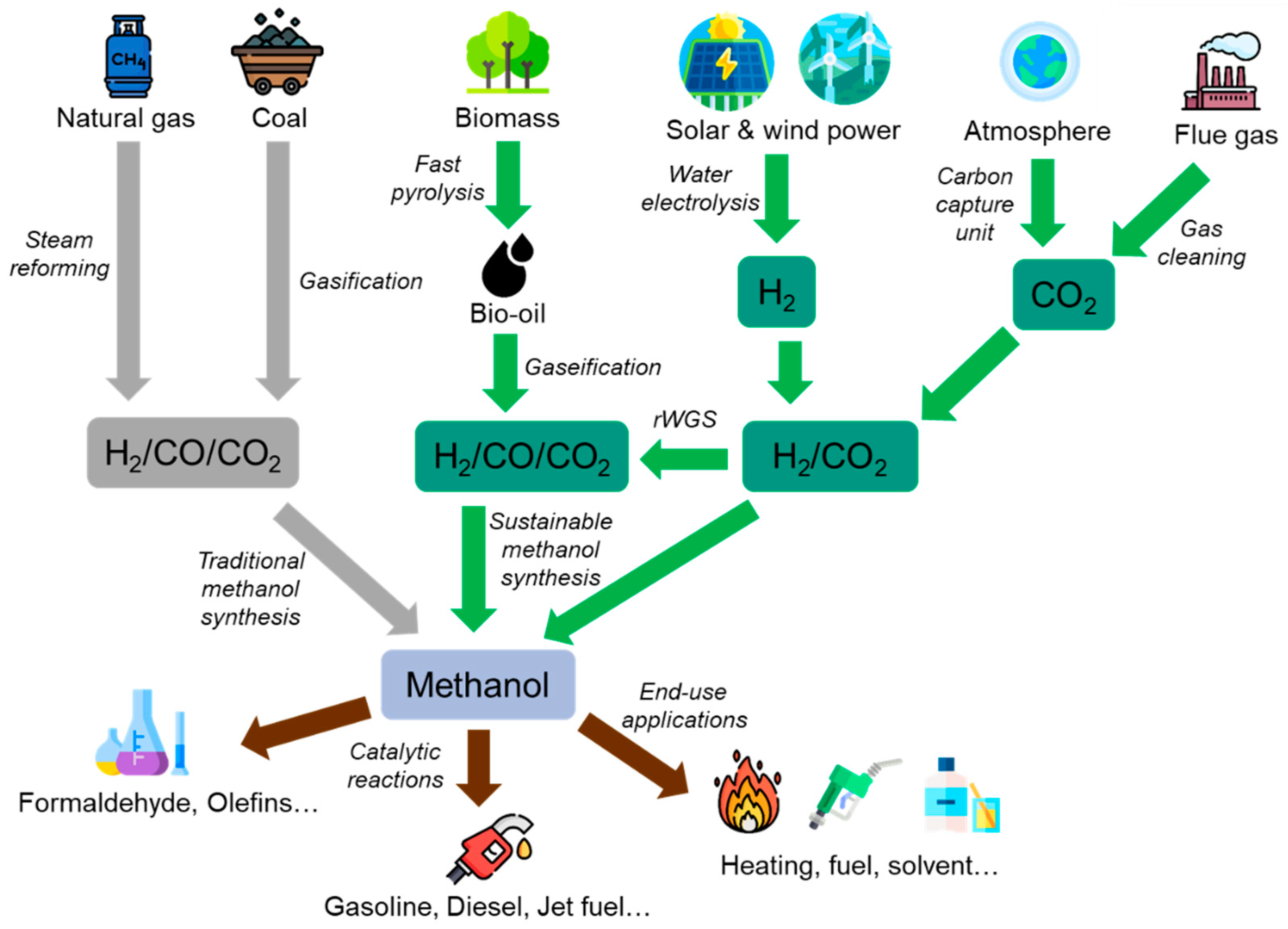
1. Introduction
2. Methodology
2.1. Process Overview
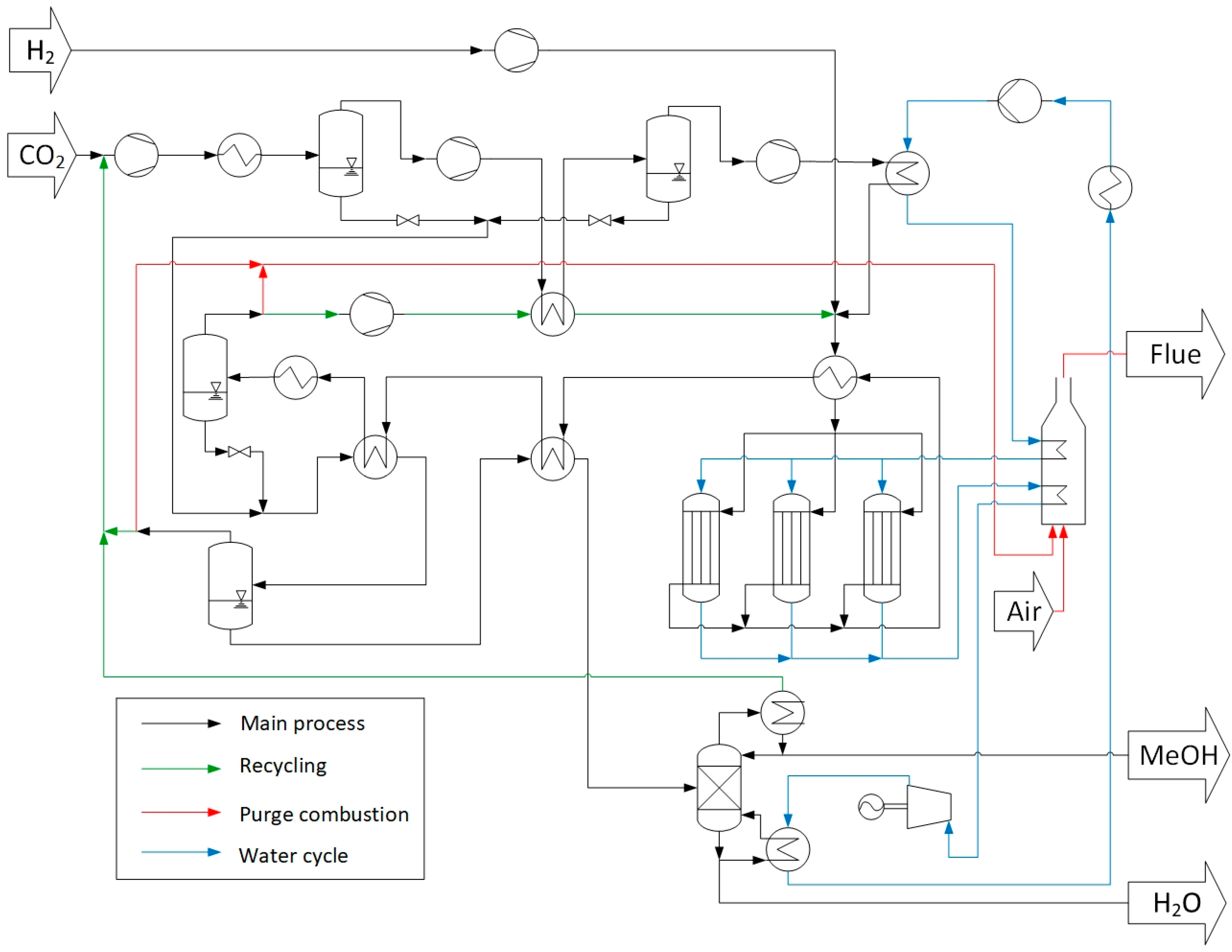
2.1.1. One-Step Approach—Process Description
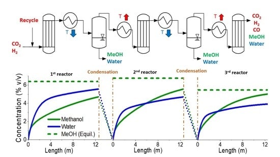
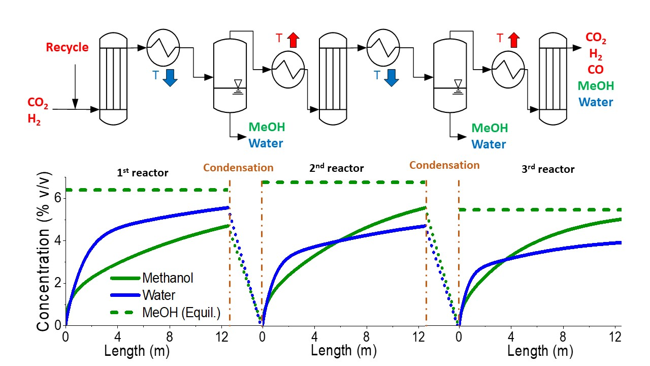
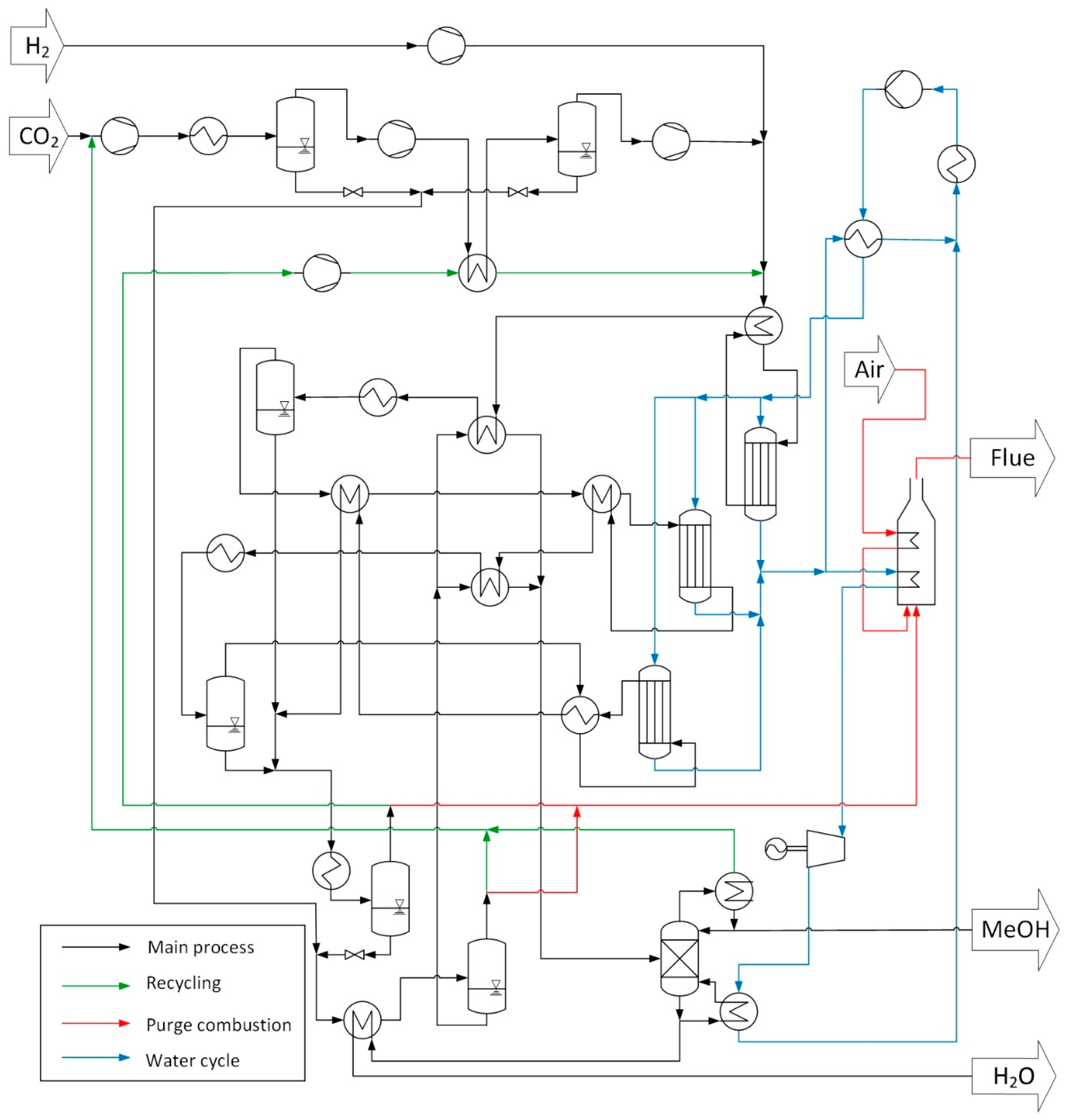
2.1.2. Three-Step Approach—Process Description
2.2. Process Simulation in Matlab
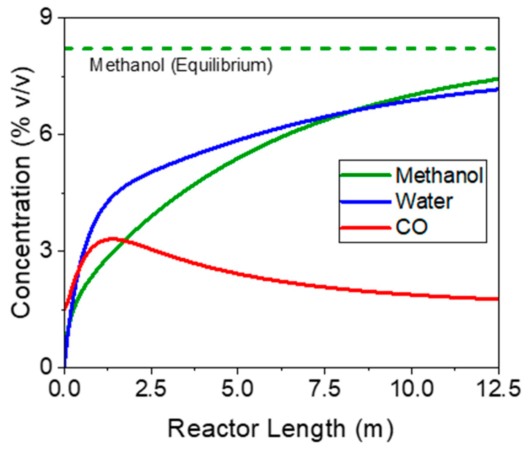
2.3. Kinetic Modeling of the Methanol Synthesis
2.4. Process Analysis and Optimization
2.5. Detailed Plant Simulation in Aspen Plus
2.6. Efficiency Evaluation
2.7. Techno-Economic Evaluation
3. Results and Discussion
3.1. One-Step Process
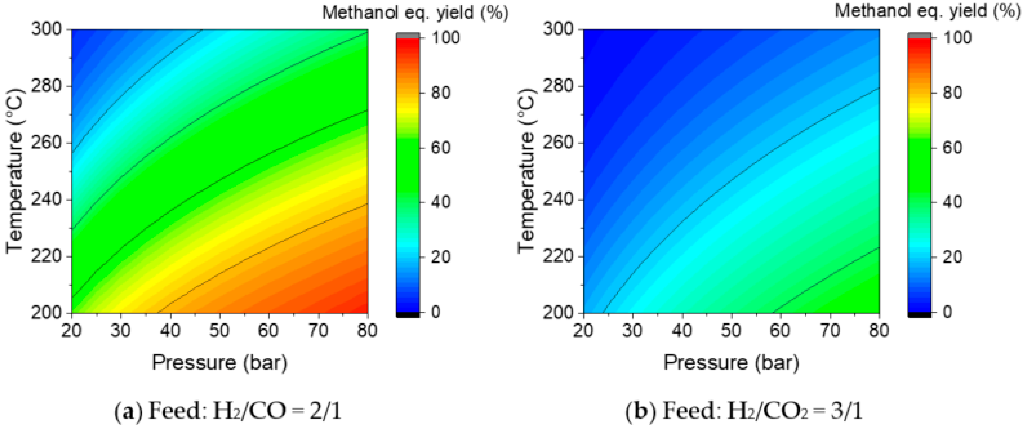
3.1.1. One-Step Process—Selecting Key Parameters
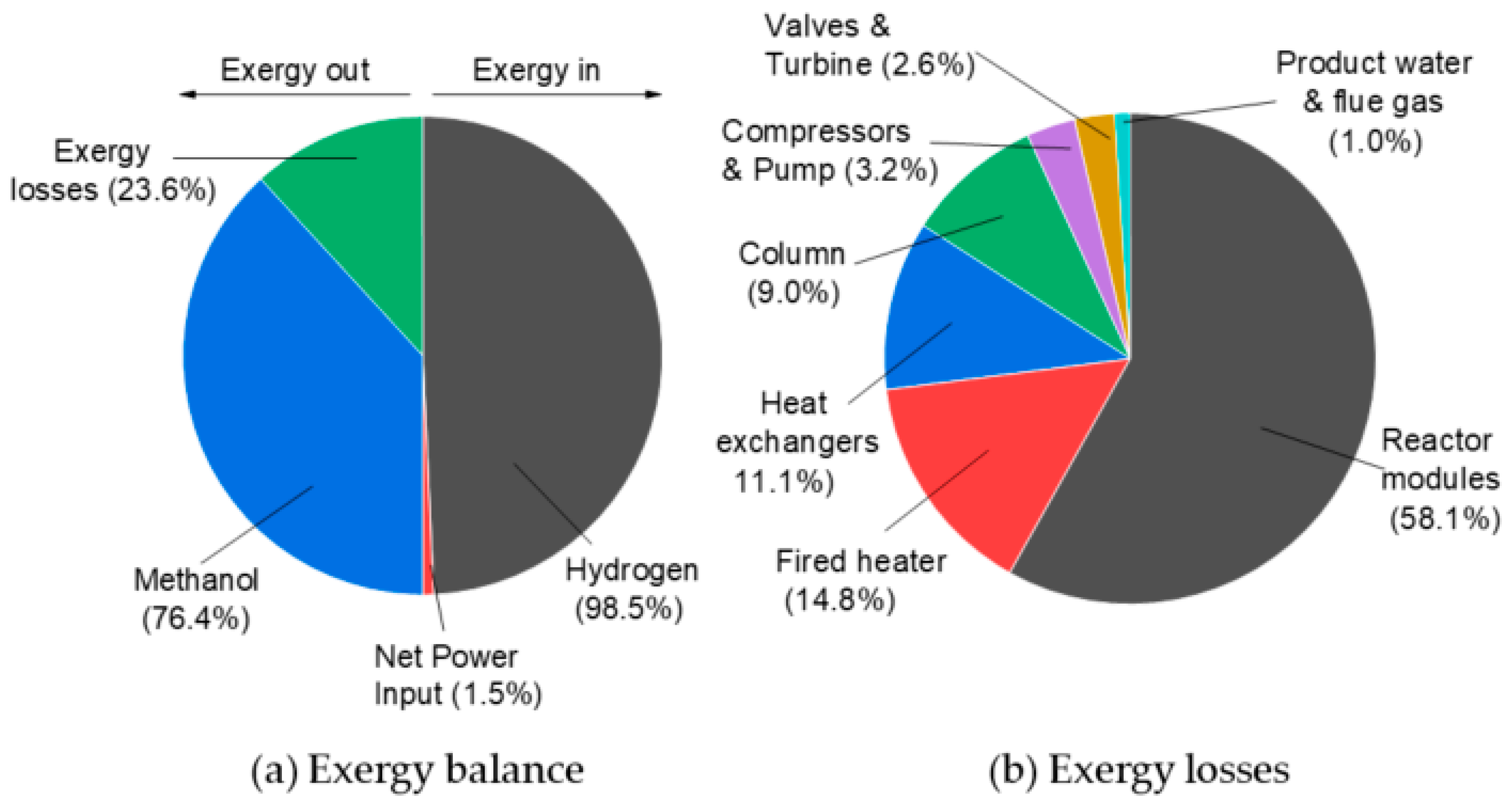
3.1.2. One-Step Process—Detailed Plant Simulation and Process Analysis
3.2. Three-Step Process
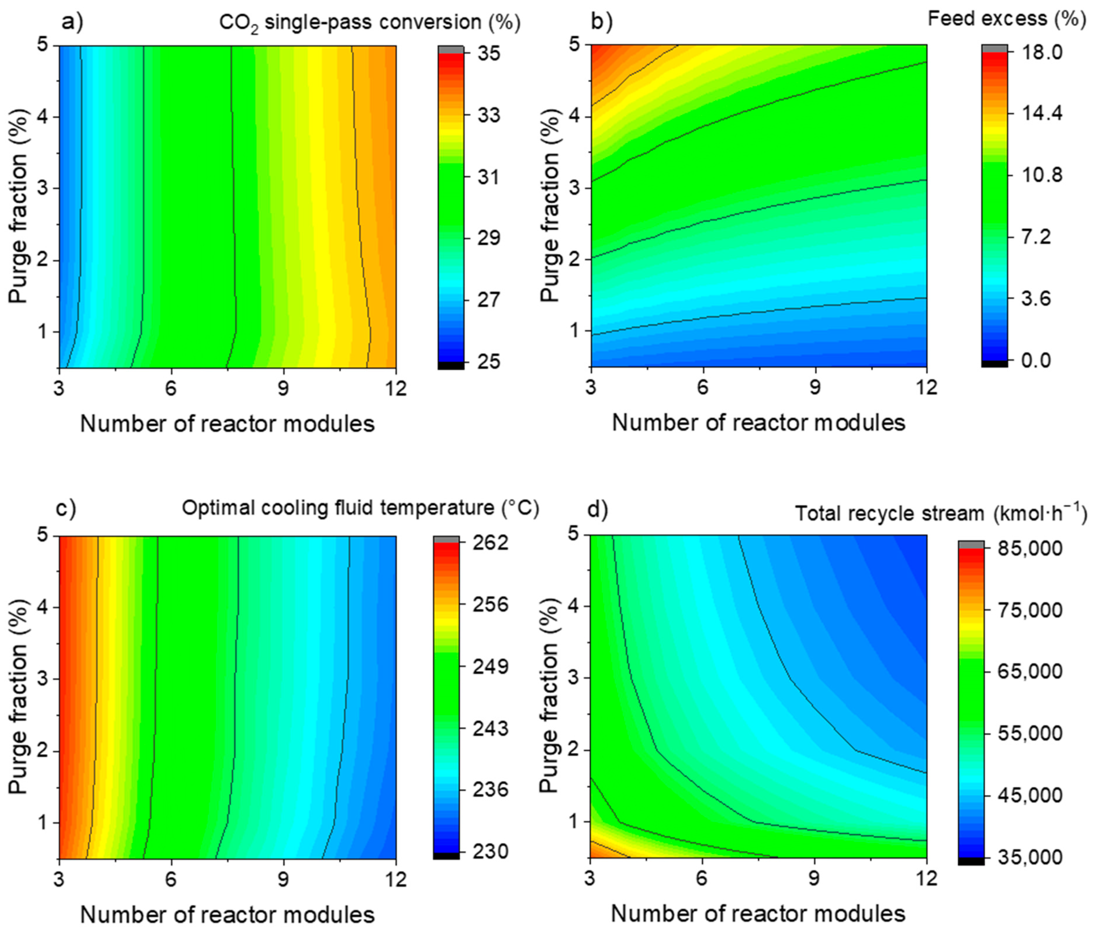
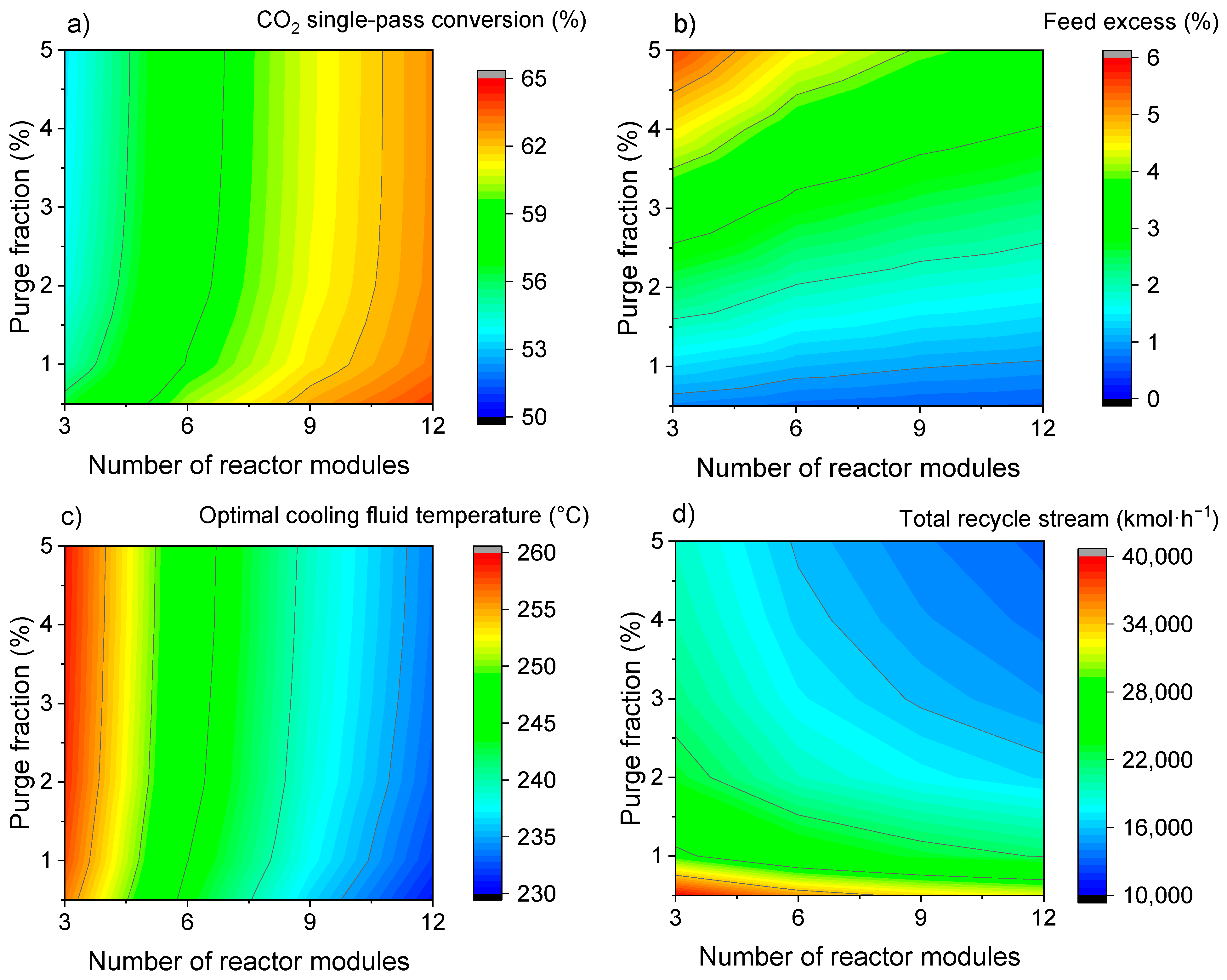
3.2.1. Three-Step Process—Selecting Key Parameters
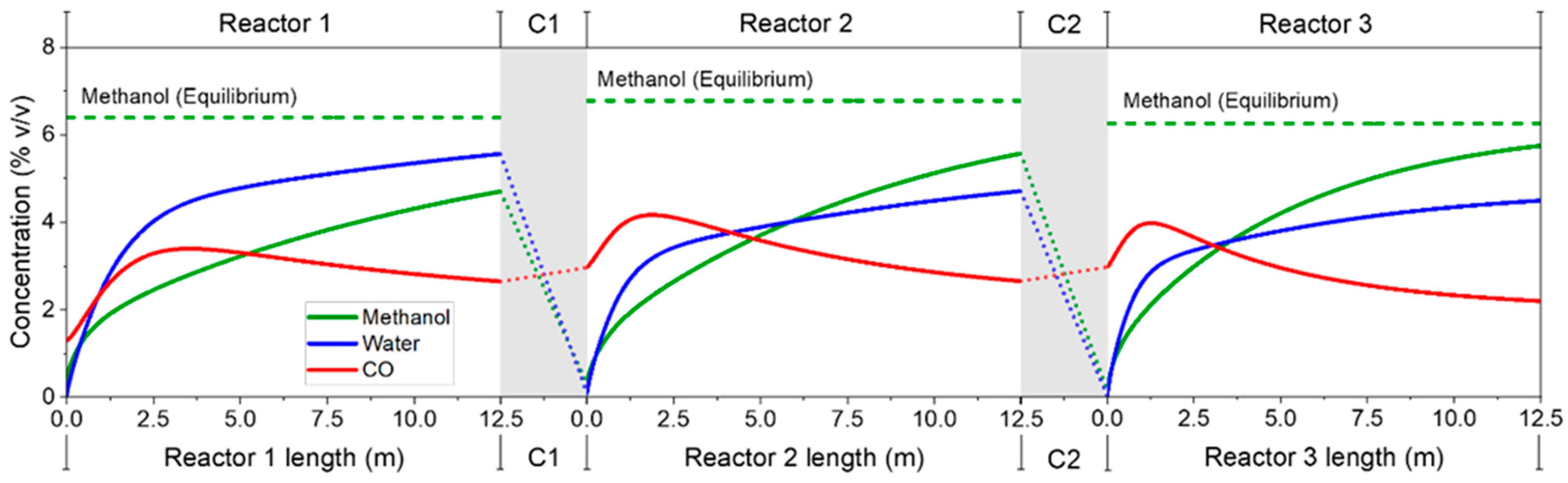
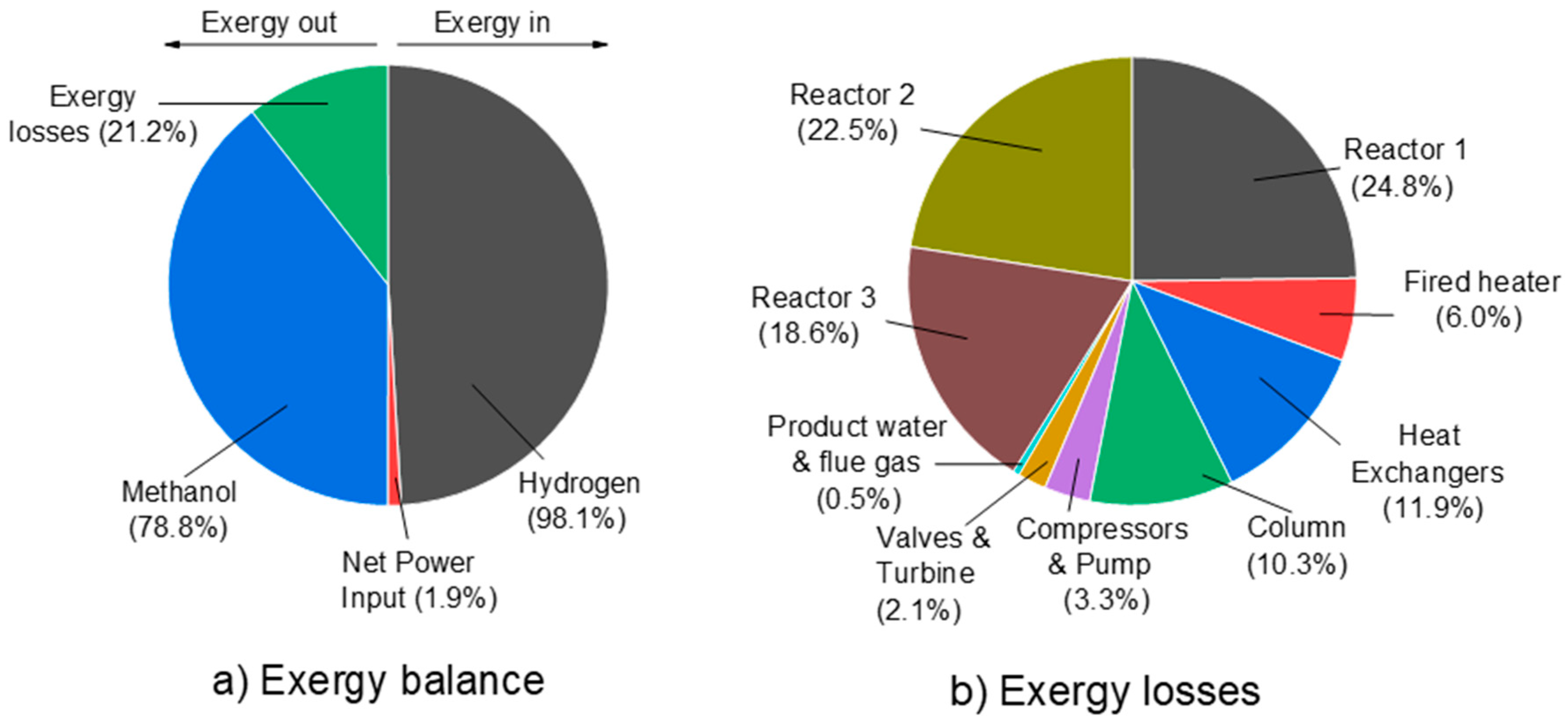
3.2.2. Three-Step Process—Detailed Plant Simulation and Process Analysis
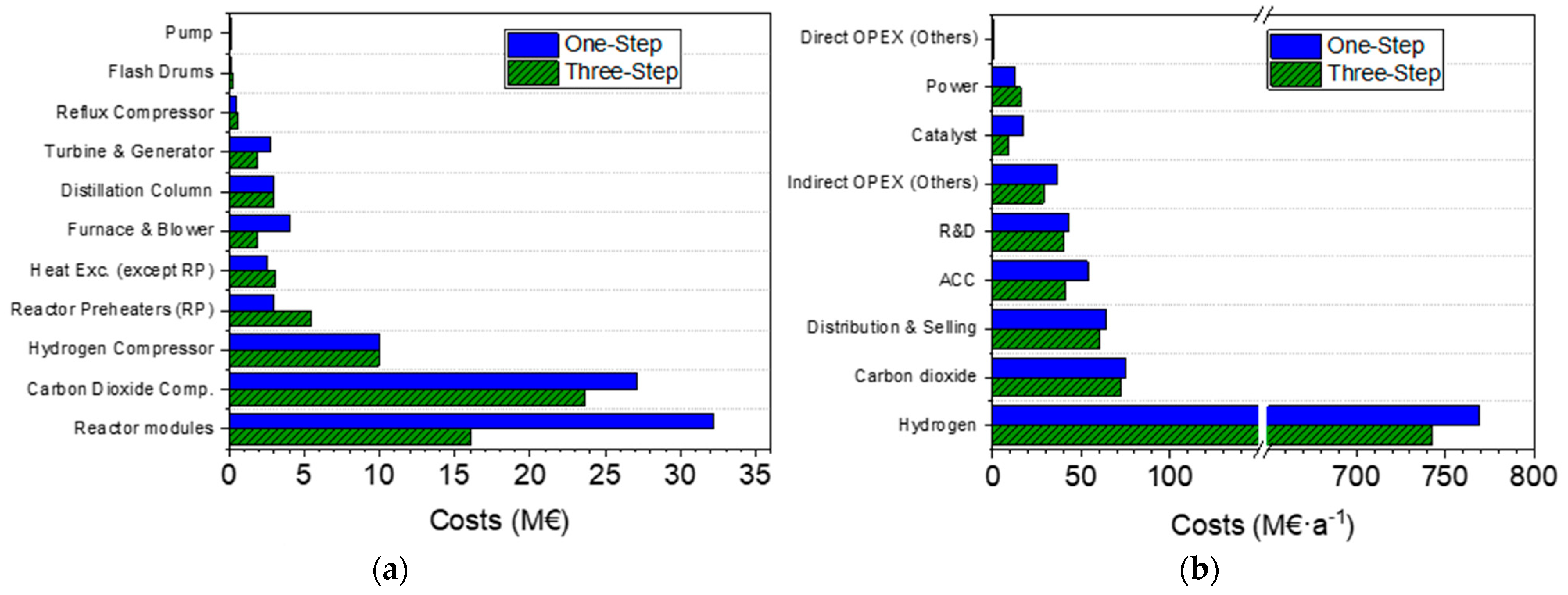
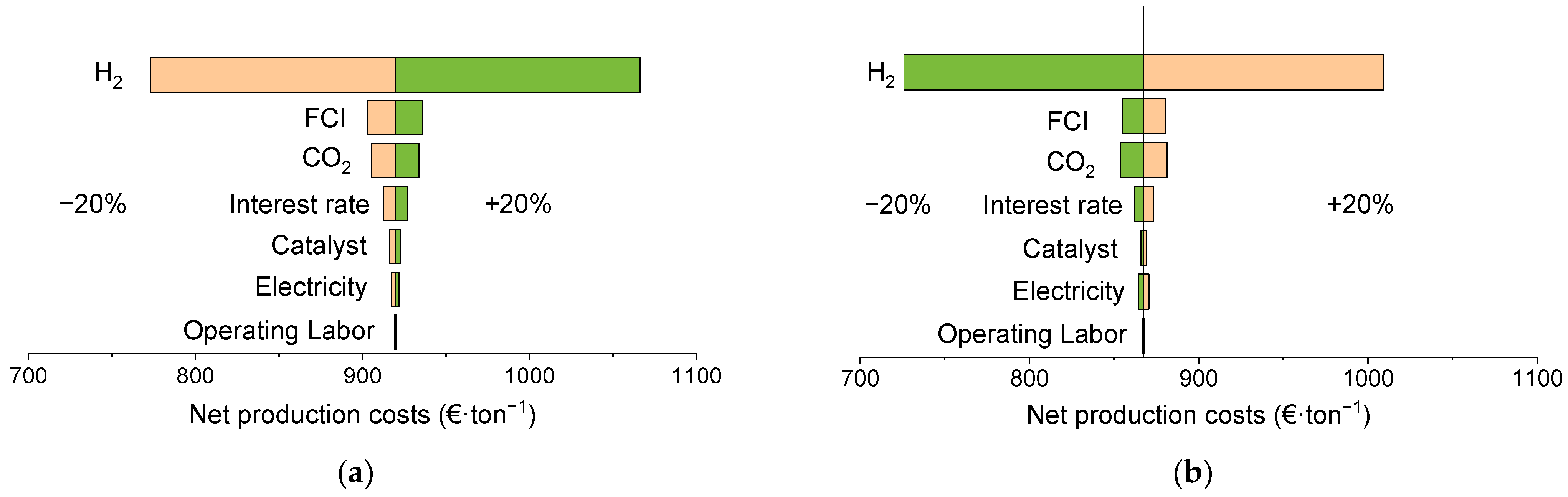
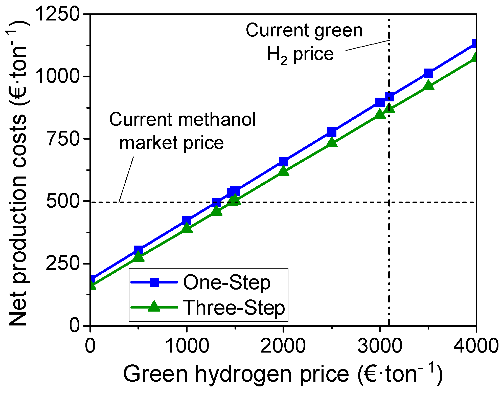
3.3. Techno-Economic Analysis
4. Conclusions
Supplementary Materials
Author Contributions
Funding
Conflicts of Interest
References
- Our World in Data. Renewable Energy. Available online: https://ourworldindata.org/renewable-energy (accessed on 4 April 2022).
- Daiyan, R.; MacGill, I.; Amal, R. Opportunities and challenges for renewable power-to-X. ACS Energy Lett. 2020, 5, 3843–3847. [Google Scholar] [CrossRef]
- Younas, M.; Shafique, S.; Hafeez, A.; Javed, F.; Rehman, F. An overview of hydrogen production: Current status, potential, and challenges. Fuel 2022, 316, 123317. [Google Scholar] [CrossRef]
- Chisholm, G.; Zhao, T.; Cronin, L. 24—Hydrogen from water electrolysis. In Storing Energy, 2nd ed.; Letcher, T.M., Ed.; Elsevier: Amsterdam, The Netherlands, 2022; pp. 559–591. [Google Scholar] [CrossRef]
- Artz, J.; Müller, T.E.; Thenert, K.; Kleinekorte, J.; Meys, R.; Sternberg, A.; Bardow, A.; Leitner, W. Sustainable conversion of carbon dioxide: An integrated review of catalysis and life cycle assessment. Chem. Rev. 2018, 118, 434–504. [Google Scholar] [CrossRef] [PubMed]
- Wang, L.; Chen, M.; Küngas, R.; Lin, T.-E.; Diethelm, S.; Maréchal, F.; Van Herle, J. Power-to-fuels via solid-oxide electrolyzer: Operating window and techno-economics. Renew. Sustain. Energy Rev. 2019, 110, 174–187. [Google Scholar] [CrossRef]
- Bongartz, D.; Burre, J.; Ziegler, A.L.; Mitsos, A. Power-to-OME1 via direct oxidation of methanol: Process design and global flowsheet optimization. In Computer Aided Chemical Engineering; Türkay, M., Gani, R., Eds.; Elsevier: Amsterdam, The Netherlands, 2021; Volume 50, pp. 273–278. [Google Scholar]
- Schmidt, P.; Batteiger, V.; Roth, A.; Weindorf, W.; Raksha, T. Power-to-liquids as renewable fuel option for aviation: A review. Chem. Ing. Tech. 2018, 90, 127–140. [Google Scholar] [CrossRef]
- Methanol Institute—Methanol Fuel in China 2020. Available online: https://www.methanol.org/methanol-fuel-in-china-full-report/ (accessed on 5 July 2022).
- Global Data—Methanol Market Capacity 2021. Available online: https://www.globaldata.com/store/report/methanol-market-analysis/ (accessed on 27 June 2022).
- Bozzano, G.; Manenti, F. Efficient methanol synthesis: Perspectives, technologies and optimization strategies. Prog. Energy Combust. Sci. 2016, 56, 71–105. [Google Scholar] [CrossRef]
- Freepik. Flaticon Icons. Available online: https://www.flaticon.com/authors/freepik (accessed on 27 June 2022).
- Ott, J.; Gronemann, V.; Pontzen, F.; Fiedler, E.; Grossmann, G.; Kersebohm, D.B.; Weiss, G.; Witte, C. Methanol. In Ullmann’s Encyclopedia of Industrial Chemistry; Wiley: New York, NY, USA, 2012. [Google Scholar] [CrossRef]
- Toyo Engineering. G-Methanol. Available online: https://www.toyo-eng.com/jp/en/solution/g-methanol/ (accessed on 9 May 2022).
- Lacerda de Oliveira Campos, B.; Herrera Delgado, K.; Wild, S.; Studt, F.; Pitter, S.; Sauer, J. Surface reaction kinetics of the methanol synthesis and the water gas shift reaction on Cu/ZnO/Al2O3. React. Chem. Eng. 2021, 6, 868–887. [Google Scholar] [CrossRef]
- Studt, F.; Behrens, M.; Kunkes, E.L.; Thomas, N.; Zander, S.; Tarasov, A.; Schumann, J.; Frei, E.; Varley, J.B.; Abild-Pedersen, F.; et al. The mechanism of CO and CO2 hydrogenation to methanol over Cu-based catalysts. ChemCatChem 2015, 7, 1105–1111. [Google Scholar] [CrossRef] [Green Version]
- Bussche, K.M.V.; Froment, G.F. A steady-state kinetic model for methanol synthesis and the water gas shift reaction on a commercial Cu/ZnO/Al2O3Catalyst. J. Catal. 1996, 161, 1–10. [Google Scholar] [CrossRef]
- Slotboom, Y.; Bos, M.J.; Pieper, J.; Vrieswijk, V.; Likozar, B.; Kersten, S.R.A.; Brilman, D.W.F. Critical assessment of steady-state kinetic models for the synthesis of methanol over an industrial Cu/ZnO/Al2O3 catalyst. Chem. Eng. J. 2020, 389, 124181. [Google Scholar] [CrossRef]
- Lacerda de Oliveira Campos, B.; Herrera Delgado, K.; Pitter, S.; Sauer, J. Development of consistent kinetic models derived from a microkinetic model of the methanol synthesis. Ind. Eng. Chem. Res. 2021, 60, 15074–15086. [Google Scholar] [CrossRef]
- Pérez-Fortes, M.; Schöneberger, J.C.; Boulamanti, A.; Tzimas, E. Methanol synthesis using captured CO2 as raw material: Techno-economic and environmental assessment. Appl. Energy 2016, 161, 718–732. [Google Scholar] [CrossRef]
- Szima, S.; Cormos, C.-C. Improving methanol synthesis from carbon-free H2 and captured CO2: A techno-economic and environmental evaluation. J. CO2 Util. 2018, 24, 555–563. [Google Scholar] [CrossRef]
- Cordero-Lanzac, T.; Ramirez, A.; Navajas, A.; Gevers, L.; Brunialti, S.; Gandía, L.M.; Aguayo, A.T.; Mani Sarathy, S.; Gascon, J. A techno-economic and life cycle assessment for the production of green methanol from CO2: Catalyst and process bottlenecks. J. Energy Chem. 2022, 68, 255–266. [Google Scholar] [CrossRef]
- FFE München. Electrolysis, the Key Technology for Power-to-X. Available online: https://www.ffe.de/veroeffentlichungen/elektrolyse-die-schluesseltechnologie-fuer-power-to-x/ (accessed on 4 April 2022).
- Fasihi, M.; Efimova, O.; Breyer, C. Techno-economic assessment of CO2 direct air capture plants. J. Clean. Prod. 2019, 224, 957–980. [Google Scholar] [CrossRef]
- Carbon Recycling International. Renewable Methanol from Carbon Dioxide. Available online: https://www.carbonrecycling.is/ (accessed on 4 April 2022).
- Siemens Energy. The Haru Oni Hydrogen Plant. Available online: https://www.siemens-energy.com/global/en/news/magazine/2021/haru-oni.html (accessed on 1 February 2022).
- van Bennekom, J.G.; Venderbosch, R.H.; Winkelman, J.G.M.; Wilbers, E.; Assink, D.; Lemmens, K.P.J.; Heeres, H.J. Methanol synthesis beyond chemical equilibrium. Chem. Eng. Sci. 2013, 87, 204–208. [Google Scholar] [CrossRef]
- Bos, M.J.; Brilman, D.W.F. A novel condensation reactor for efficient CO2 to methanol conversion for storage of renewable electric energy. Chem. Eng. J. 2015, 278, 527–532. [Google Scholar] [CrossRef] [Green Version]
- Seshimo, M.; Liu, B.; Lee, H.R.; Yogo, K.; Yamaguchi, Y.; Shigaki, N.; Mogi, Y.; Kita, H.; Nakao, S.-i. Membrane reactor for methanol synthesis using Si-Rich LTA Zeolite Membrane. Membranes 2021, 11, 505. [Google Scholar] [CrossRef]
- Johnson Mattey. Methanol Synthesis Technology. Available online: https://matthey.com/en/products-and-services/chemical-processes/core-technologies/synthesis (accessed on 9 May 2022).
- Guo, Y.; Li, G.; Zhou, J.; Liu, Y. Comparison between hydrogen production by alkaline water electrolysis and hydrogen production by PEM electrolysis. IOP Conf. Ser. Earth Environ. Sci. 2019, 371, 042022. [Google Scholar] [CrossRef]
- Porter, R.T.J.; Fairweather, M.; Kolster, C.; Mac Dowell, N.; Shah, N.; Woolley, R.M. Cost and performance of some carbon capture technology options for producing different quality CO2 product streams. Int. J. Greenh. Gas Control. 2017, 57, 185–195. [Google Scholar] [CrossRef]
- Bennekom, J.G.v.; Winkelman, J.G.M.; Venderbosch, R.H.; Nieland, S.D.G.B.; Heeres, H.J. Modeling and experimental studies on phase and chemical equilibria in high-pressure methanol synthesis. Ind. Eng. Chem. Res. 2012, 51, 12233–12243. [Google Scholar] [CrossRef]
- Gaikwad, R.; Bansode, A.; Urakawa, A. High-pressure advantages in stoichiometric hydrogenation of carbon dioxide to methanol. J. Catal. 2016, 343, 127–132. [Google Scholar] [CrossRef] [Green Version]
- Süd-Chemie AG. Safety Data Sheet—MegaMax 700. 2006. [Google Scholar]
- Zhu, J.; Araya, S.S.; Cui, X.; Sahlin, S.L.; Kær, S.K. Modeling and design of a multi-tubular packed-bed reactor for methanol steam reforming over a Cu/ZnO/Al2O3 Catalyst. Energies 2020, 13, 610. [Google Scholar] [CrossRef] [Green Version]
- Van-Dal, É.S.; Bouallou, C. Design and simulation of a methanol production plant from CO2 hydrogenation. J. Clean. Prod. 2013, 57, 38–45. [Google Scholar] [CrossRef]
- Pontzen, F.; Liebner, W.; Gronemann, V.; Rothaemel, M.; Ahlers, B. CO2-based methanol and DME—Efficient technologies for industrial scale production. Catal. Today 2011, 171, 242–250. [Google Scholar] [CrossRef]
- Bongartz, D.; Burre, J.; Mitsos, A. Production of oxymethylene dimethyl ethers from hydrogen and carbon dioxide—Part I: Modeling and analysis for OME1. Ind. Eng. Chem. Res. 2019, 58, 4881–4889. [Google Scholar] [CrossRef]
- Burners for Fired Heaters in General Refinery Services. In Reference Practice (RP) 535, 3rd ed.; American Petroleum Institute (API): Washington, DC, USA, 2014.
- Goos, E.; Burcat, A.; Ruscic, B. New NASA Thermodynamic Polynomials Database. Available online: http://garfield.chem.elte.hu/Burcat/THERM.DAT (accessed on 4 March 2022).
- Gruber, M. Detaillierte Untersuchung des Wärme und Stofftransports in einem Festbett-Methanisierungsreaktor für Power-to-Gas Anwendungen. Ph.D. Thesis, Karlsruhe Institute of Technology (KIT), Karlsruhe, Germany, 2019; 275p. [Google Scholar]
- VDI Heat Atlas, 2nd ed.; Springer: Berlin-Heidelberg, Germany, 2010; p. 1585.
- Seidel, C.; Jörke, A.; Vollbrecht, B.; Seidel-Morgenstern, A.; Kienle, A. Kinetic modeling of methanol synthesis from renewable resources. Chem. Eng. Sci. 2018, 175, 130–138. [Google Scholar] [CrossRef] [Green Version]
- Peng, D.-Y.; Robinson, D.B. A new two-constant equation of State. Ind. Eng. Chem. Fundam. 1976, 15, 59–64. [Google Scholar] [CrossRef]
- Meng, L.; Duan, Y.-Y.; Wang, X.-D. Binary interaction parameter kij for calculating the second cross-virial coefficients of mixtures. Fluid Phase Equilibria 2007, 260, 354–358. [Google Scholar] [CrossRef]
- Meng, L.; Duan, Y.-Y. Prediction of the second cross virial coefficients of nonpolar binary mixtures. Fluid Phase Equilibria 2005, 238, 229–238. [Google Scholar] [CrossRef]
- Deiters, U.K. Comments on the modeling of hydrogen and hydrogen-containing mixtures with cubic equations of state. Fluid Phase Equilibria 2013, 352, 93–96. [Google Scholar] [CrossRef]
- Kuld, S.; Thorhauge, M.; Falsig, H.; Elkjær, C.F.; Helveg, S.; Chorkendorff, I.; Sehested, J. Quantifying the promotion of Cu catalysts by ZnO for methanol synthesis. Science 2016, 352, 969–974. [Google Scholar] [CrossRef] [PubMed] [Green Version]
- CLARIANT. Catalysts for Methanol Synthesis, Product Data Sheet. 2017. Available online: https://www.clariant.com/-/media/Files/Solutions/Products/Additional-Files/M/18/Clariant-Brochure-Methanol-Synthesis-201711-EN.pdf (accessed on 4 April 2022).
- Saito, M.; Murata, K. Development of high performance Cu/ZnO-based catalysts for methanol synthesis and the water-gas shift reaction. Catal. Surv. Asia 2004, 8, 285–294. [Google Scholar] [CrossRef]
- Campos Fraga, M.M.; Lacerda de Oliveira Campos, B.; Lisboa, M.S.; Almeida, T.B.; Costa, A.O.S.; Lins, V.F.C. Analysis of a Brazilian thermal plant operation applying energetic and exergetic balances. Braz. J. Chem. Eng. 2018, 35, 1395–1403. [Google Scholar] [CrossRef] [Green Version]
- Nitzsche, R.; Budzinski, M.; Gröngröft, A. Techno-economic assessment of a wood-based biorefinery concept for the production of polymer-grade ethylene, organosolv lignin and fuel. Bioresour. Technol. 2016, 200, 928–939. [Google Scholar] [CrossRef] [PubMed]
- Green, D.W.; Southard, M.Z. Perry’s Chemical Engineers’ Handbook, 9th ed.; McGraw Hill: New York, NY, USA, 2018. [Google Scholar]
- König, D.H.; Baucks, N.; Dietrich, R.-U.; Wörner, A. Simulation and evaluation of a process concept for the generation of synthetic fuel from CO2 and H2. Energy 2015, 91, 833–841. [Google Scholar] [CrossRef] [Green Version]
- Albrecht, F.G.; König, D.H.; Baucks, N.; Dietrich, R.-U. A standardized methodology for the techno-economic evaluation of alternative fuels—A case study. Fuel 2017, 194, 511–526. [Google Scholar] [CrossRef] [Green Version]
- Peters, M.S.; Timmerhaus, K.D.; West, R.E. Plant Design and Economics for Chemical Engineers, 5th ed.; McGraw-Hill Education Ltd.: Boston, MA, USA, 2002; p. 1008. [Google Scholar]
- Hennig, M.; Haase, M. Techno-economic analysis of hydrogen enhanced methanol to gasoline process from biomass-derived synthesis gas. Fuel Processing Technol. 2021, 216, 106776. [Google Scholar] [CrossRef]
- Travelex. Worldwide Money. Available online: https://www.travelex.com/currency/currency-pairs/usd-to-eur (accessed on 4 April 2022).
- Towler, G.; Sinnott, R. Chemical Engineering Design—Principles, Practice and Economics of Plant and Process Design, 2nd ed.; Elsevier: Amsterdam, The Netherlands, 2013. [Google Scholar]
- Aden, A.; Ruth, M.; Ibsen, K.; Jechura, J.; Neeves, K.; Sheehan, J.; Wallace, B.; Montague, L.; Slayton, A.; Lukas, J. Lignocellulosic Biomass to Ethanol Process Design and Economics Utilizing Co-Current Dilute Acid Prehydrolysis and Enzymatic Hydrolysis for Corn Stover; National Renewable Energy Laboratory: Golden, CO, USA, 2002; 154p.
- Cheremisinoff, N.P. Clean Electricity Through Advanced Coal Technologies; Elsevier: Amsterdam, The Netherlands, 2012. [Google Scholar] [CrossRef]
- Bustillo-Lecompte, C.F.; Mehrvar, M.; Quiñones-Bolaños, E. Cost-effectiveness analysis of TOC removal from slaughterhouse wastewater using combined anaerobic–aerobic and UV/H2O2 processes. J. Environ. Manag. 2014, 134, 145–152. [Google Scholar] [CrossRef]
- Tan, E.C.; Talmadge, M.; Dutta, A.; Hensley, J.; Snowden-Swan, L.J.; Humbird, D.; Schaidle, J.; Biddy, M. Conceptual process design and economics for the production of high-octane gasoline blendstock via indirect liquefaction of biomass through methanol/dimethyl ether intermediates. Biofuels Bioprod. Biorefining 2016, 10, 17–35. [Google Scholar] [CrossRef]
- Ashraf, M.T.; Schmidt, J.E. Process simulation and economic assessment of hydrothermal pretreatment and enzymatic hydrolysis of multi-feedstock lignocellulose—Separate vs. combined processing. Bioresour. Technol. 2018, 249, 835–843. [Google Scholar] [CrossRef] [PubMed]
- Granjo, J.F.O.; Oliveira, N.M.C. Process simulation and techno-economic analysis of the production of sodium methoxide. Ind. Eng. Chem. Res. 2016, 55, 156–167. [Google Scholar] [CrossRef]
- Prašnikar, A.; Pavlišič, A.; Ruiz-Zepeda, F.; Kovač, J.; Likozar, B. Mechanisms of copper-based catalyst deactivation during CO2 reduction to methanol. Ind. Eng. Chem. Res. 2019, 58, 13021–13029. [Google Scholar] [CrossRef] [Green Version]
- Argus Media. European Methanol Spot and Contract Prices. Available online: https://www.argusmedia.com/en/blog/2022/february/4/european-methanol-spot-and-contract-prices (accessed on 4 April 2022).
- Methanol Institute—Methanol Prices, Supply and Demand. Available online: https://www.methanol.org/methanol-price-supply-demand/ (accessed on 4 April 2022).


| Parameter | Value | Equation | Unit |
|---|---|---|
| 14.41 ± 0.99 | – | |
| 29.13 ± 1.74 | – | |
| 94.73 ± 4.18 | kJ·mol−1 | |
| 132.79 ± 7.46 | kJ·mol−1 | |
| 0.1441 ± 0.0289 | bar−1.5 | |
| 49.44 ± 11.08 | bar−0.5 | |
| bar−2 | ||
| – |
| Item | Costs | Ref. |
|---|---|---|
| Hydrogen | 3097.4 €·ton−1 | [22] |
| Carbon dioxide | 44.3 €·ton−1 | [22] |
| Cooling water | 0.00125 €·ton−1 | [56] |
| Clean water | 2 €·ton−1 | [56] |
| Total organic carbon (TOC) abatement of process water | 1938 €·(ton C)−1 | [63] |
| Electricity | 90 €·MWh−1 | [53] |
| Catalyst (Cu/ZnO/Al2O3) | 18,100 €·ton−1 | [64] |
| Approach | (°C) | (°C) | (°C) | (%) | Feed Excess (%) | Total Recycle Stream (kmol·h−1) |
|---|---|---|---|---|---|---|
| 258.5 | 258.5 | 258.5 | 54.1 | 2.42 | 23,038 | |
| 264.6 | 259.9 | 249.4 | 54.6 | 2.35 | 22,464 |
| Cond. Step | Temp. (°C) | Pres. (Bar) | Phase | Split Ratio | ||
|---|---|---|---|---|---|---|
| CO2 (%) | MeOH (%) | H2O (%) | ||||
| #1 | 45 | 69.25 | Gas | 90.66 | 5.31 | 1.17 |
| Liquid | 9.34 | 94.69 | 98.83 | |||
| #2 | 30 | 68.50 | Gas | 87.36 | 2.46 | 0.52 |
| Liquid | 12.64 | 97.54 | 99.48 | |||
| Reactor | #1 | #2 | #3 |
|---|---|---|---|
| (MW) | −18.5 | −25.7 | −22.7 |
| (kmol·h−1) | 40,833 | 33,209 | 26,366 |
| (% mol/mol) | 69.1 | 69.0 | 69.5 |
| (% mol/mol) | 1.3 | 3.0 | 3.0 |
| (% mol/mol) | 20.6 | 17.3 | 14.4 |
| (% mol/mol) | 4.7 | 5.6 | 5.8 |
| (% mol/mol) | 5.6 | 4.7 | 4.5 |
| (kmol·h−1) | 1616 | 1589 | 1325 |
| Item | One-Step | Three-Step |
|---|---|---|
| Total methanol production (kmol·h−1) | 4527 | 4525 |
| CO2 single-pass conversion (%) | 28.5 | 53.9 |
| Overall CO2 conversion to methanol (%) | 94.3 | 97.7 |
| Feed excess (%) | 6.05 | 2.35 |
| Methanol selectivity (%) | 99.5 | 99.8 |
| Total recycle stream flow (kmol·h−1) | 54,290 | 22,581 |
| Maximum water concentration (% mol/mol) | 7.2 | 5.6 |
| Total exergy loss (MW) | 281.9 | 245.3 |
| Exergy efficiency (%) | 76.4 | 78.8 |
| Item | Costs | Decrease (%) | |
|---|---|---|---|
| One-Step | Three-Step | ||
| ) | 85.5 M€ | 66.1 M€ | 22.7 |
| ) | 415.9 M€ | 321.4 M€ | 22.7 |
| ) | 46.2 M€ | 35.7 M€ | 22.7 |
| 462.1 M€ | 357.1 M€ | 22.7 | |
| ) | 53.5 M€·a−1 | 41.3 M€·a−1 | 22.7 |
| 874.9 M€·a−1 | 839.6 M€·a−1 | 4.0 | |
| 143.4 M€·a−1 | 129.6 M€·a−1 | 9.6 | |
| 1018.3 M€·a−1 | 969.3 M€·a−1 | 4.8 | |
| ) | 1071.8 M€·a−1 | 1010.6 M€·a−1 | 5.7 |
Publisher’s Note: MDPI stays neutral with regard to jurisdictional claims in published maps and institutional affiliations. |
© 2022 by the authors. Licensee MDPI, Basel, Switzerland. This article is an open access article distributed under the terms and conditions of the Creative Commons Attribution (CC BY) license (https://creativecommons.org/licenses/by/4.0/).
Share and Cite
Lacerda de Oliveira Campos, B.; John, K.; Beeskow, P.; Herrera Delgado, K.; Pitter, S.; Dahmen, N.; Sauer, J. A Detailed Process and Techno-Economic Analysis of Methanol Synthesis from H2 and CO2 with Intermediate Condensation Steps. Processes 2022, 10, 1535. https://doi.org/10.3390/pr10081535
Lacerda de Oliveira Campos B, John K, Beeskow P, Herrera Delgado K, Pitter S, Dahmen N, Sauer J. A Detailed Process and Techno-Economic Analysis of Methanol Synthesis from H2 and CO2 with Intermediate Condensation Steps. Processes. 2022; 10(8):1535. https://doi.org/10.3390/pr10081535
Chicago/Turabian StyleLacerda de Oliveira Campos, Bruno, Kelechi John, Philipp Beeskow, Karla Herrera Delgado, Stephan Pitter, Nicolaus Dahmen, and Jörg Sauer. 2022. "A Detailed Process and Techno-Economic Analysis of Methanol Synthesis from H2 and CO2 with Intermediate Condensation Steps" Processes 10, no. 8: 1535. https://doi.org/10.3390/pr10081535