Mobile Robot Navigation Using Deep Reinforcement Learning

Abstract

Learning how to navigate autonomously in an unknown indoor environment without colliding with static and dynamic obstacles is important for mobile robots. The conventional mobile robot navigation system does not have the ability to learn autonomously. Unlike conventional approaches, this paper proposes an end-to-end approach that uses deep reinforcement learning for autonomous mobile robot navigation in an unknown environment. Two types of deep Q-learning agents, such as deep Q-network and double deep Q-network agents are proposed to enable the mobile robot to autonomously learn about collision avoidance and navigation capabilities in an unknown environment. For autonomous mobile robot navigation in an unknown environment, the process of detecting the target object is first carried out using a deep neural network model, and then the process of navigation to the target object is followed using the deep Q-network or double deep Q-network algorithm. The simulation results show that the mobile robot can autonomously navigate, recognize, and reach the target object location in an unknown environment without colliding with static and dynamic obstacles. Similar results are obtained in real-world experiments, but only with static obstacles. The DDQN agent outperforms the DQN agent in reaching the target object location in the test simulation by 5.06%.

1. Introduction

Robots play an important role in our daily lives, such as rescuing, cleaning, medical assisting, helping military operations, working in hazardous operations, and autonomous driving. Most of the above applications require mobile robots to navigate in an unknown environment without colliding with static and dynamic obstacles. Navigation is the mechanism by which a mobile robot moves to perform a certain task in the environment. Autonomous navigation is carried out when the robot moves in an environment without any intervention from an external controller (e.g., a human). Autonomous navigation is one of the key research topics in the field of mobile robotics [1]. Benefiting from the advancement of artificial intelligence (AI) and computer vision, enormous developments have been made in autonomous mobile robot navigation [2,3]. However, it still remains a difficult challenge to enable mobile robots to autonomously navigate in the real world.

The conventional navigation method (i.e., map-building-based navigation) consists of localization, map building, and path planning (e.g., simultaneous localization and mapping (SLAM)) [4]. Using a map has many advantages since the entire planning and control system becomes computationally tractable by projecting high-dimensional observation, such as a camera image, into a three-dimensional pose on the map. In addition, it is possible to conveniently guarantee the optimality of the global path, however, it also has some drawbacks. First, creating an accurate environmental map is time- and labor-consuming and often requires expert knowledge. Second, from a long-term perspective, maintaining and updating the map can be much more costly, particularly in the face of dynamic changes. Third, the efficiency of the control depends solely on the robot’s mathematical model, which, however, is typically simplified or linearized and this ultimately weakens the navigation system’s robustness. Unlike map-building-based navigation, mapless navigation as an alternative is more commonly regarded as a solution to alleviate a map’s prerequisite from the navigation system as it generally models a direct mapping between sensory inputs and robot actions. Unfortunately, without a map, it is incredibly difficult to plan the global path for the optimal path. Therefore, mapless navigation is more frequently applied in tasks without explicit destinations, e.g., collision avoidance, or with a known destination in the robot’s local coordinate frame. Thus, in this context, mapless navigation is similar to behavior-based navigation [5] which has no high-level reasoning process based on environmental prior knowledge. In the last four years, the popularity of deep reinforcement learning (DRL) has increased dramatically. It began with two success stories through the combination of reinforcement learning (RL) with deep neural networks (DNNs) achieving impressive and exciting results.

First, a single RL agent was developed by the DeepMind community that was able to play several human-level Atari 2600 video games [6]. An action is selected from several discrete actions based on raw input images of the game, while the game’s score serves as the reward. This implemented method is well-known as a deep Q-network (DQN), which uses a DNN as a Q-learning function approximator and solves the problem of instability. AlphaGo [7] is the second success story developed by the DeepMind community for the Chinese board game Go, which was able to defeat the world champion. AlphaGo is trained by a novel combination of supervised learning and RL. For robotics, DRL has been shown to be able to master complicated tasks such as Go [7] and digest observations from various domains, e.g., raw input [8] and laser scans [9]. Using DRL for robotics is still challenging, however, in recent years, DRL has been applied in various robotic fields, such as robotic manipulation [10,11,12], locomotion [13,14], self-driving vehicles [15,16], and autonomous navigation [17]. RL requires millions of experiences to properly learn complex tasks. Therefore, most RL-based mobile robots cannot be trained from real-world samples as robotic hardware is expensive and vulnerable to damage. As a result, conducting the training process in a simulator and then transferring the trained methodology to real-world scenarios is a more practical option [9,18]. The practical implementation of DRL in real robotic tasks poses significant problems. Thus, the ultimate objective of this paper is to find solutions to these problems, with the vision of delivering practical DRL methods for autonomous navigation that are efficient for training, generalizable, and capable of being deployed on real mobile robots. This paper is structured as follows. The second section introduces the related work. The third section discusses the method and materials. The fourth and fifth sections present the experiment’s results and discussions. Finally, the sixth section is the conclusion of this study.

2. Related Work

An algorithm for solving the SLAM problem has been proposed in [19], which is a critical problem for mobile robot autonomous navigation in an unknown environment. OrthoSLAM [20] is a lightweight and real-time efficient SLAM algorithm for a minimum system embedded in simple mobile robots for indoor office-like environments. It attempts to reduce the complexity by assuming the lines in the environment structure are parallel or perpendicular to each other. A novel method, which is a combination of the Hector SLAM and the artificial potential field (APF) controller, for the autonomous indoor navigation of a wheeled mobile robot (i.e., global positioning system (GPS) denied environment typical for a greenhouse), was proposed in [21]. The robot uses single light detection and ranging (LiDAR) for localization, an open-source Hector SLAM for pose estimation, and an APF controller for autonomous navigation. A semantically rich graph representation was proposed for indoor robotic navigation in [22], where the navigational tasks operate directly from the semantic information to generate motor commands. This enables the robot to avoid explicit computation for its precise location or the geometry of the environment. However, the method is not implemented using a real robot. An end-to-end approach to train the convolutional neural network (CNN) model for autonomous mobile robot navigation using an RGB−D camera only was proposed in [23]. A navigation method to learn the end-to-end control policy using the CNN model to directly generate the velocity and angular rates from the current observation and target was proposed in [24]. Nevertheless, these last two approaches [23,24] consisted of learning behavior with labeled observation, but not learning from the environment itself, as well as it requires a lot of labeling and does not do well in generalization.

A novel method for mobile robot navigation using a DRL was proposed in [25]. This approach is based on deep reinforcement learning and recurrent neural network (RNN), which combines double net and RNN modules with reinforcement learning ideas. Here, the DRL is used to make decisions after training based on the path selection of the agent from one location to another. Deep reinforcement learning for autonomous mobile robot navigation based on a deep Q-network (DQN) was proposed in [26]. The method is concerned with the autonomous navigation of mobile robots from the current position to the desired position using only a current visual observation. Due to the usage of an RGB−D camera, the method is limited in its ability to perceive the environment. A deep reinforcement learning approach to enable the mobile robot to learn autonomous navigation capabilities and collision avoidance based on a double deep Q-network (DDQN) was proposed in [27,28]. Information such as the size and position of the obstacle and the target position are taken as input and the robot’s direction of motion is taken as output. A deep reinforcement learning approach for autonomous mobile robot navigation using an asynchronous advantage actor–critic network in an indoor environment was proposed in [29]. The approach introduces a parallel environment simulation for mobile robots into the deep reinforcement learning process to improve generalization, avoid overfitting, and reduce the learning process time.

The purpose of this paper is to design autonomous mobile robot navigation trained by a DRL algorithm; a branch of machine learning focused on selecting actions to optimize environmental rewards (the science of optimizing problem-solving efficiency based on experience). RL is a goal-oriented cognitive approach where an agent learns to execute a task by interacting with an unknown environment. This learning approach encourages an agent to make a variety of decisions without human interference to optimize the total reward for the task and without being directly programmed to accomplish the task. First, the agents learned in the Gazebo training simulation environment. Next, the trained DQN and DDQN policies are evaluated in the Gazebo testing environment using pre-trained weights. Finally, the evaluated DQN and DDQN policies are directly deployed to the real mobile robot without modification in the algorithm. The mobile robot requires a lot of training iterations in the Gazebo simulation environment before it can reach the goal location and avoid collisions successfully. The problem statement is to train DQN and DDQN agents to learn an optimal policy to autonomously navigate mobile robots in an unknown environment.

In contrast to SLAM, an extension of the method in [28] and an end-to-end DRL approach are proposed for the autonomous navigation of mobile robots in an unknown environment without colliding with static and dynamic obstacles. The primary contribution is to provide a model-free (no need for kinematics and dynamics mobile robot equations) DRL approach for autonomous mobile robot navigation problems. Moreover, it also extends the work in [28], i.e., the addition of an RGB−D camera for detecting the target object and the deployment of the algorithm into a real mobile robot without hyperparameters tuning. The experimental results show the proposed DRL algorithm can navigate mobile robots autonomously in an unknown environment without colliding with static and dynamic obstacles.

3. Materials and Methods

Robot navigation is a classic robotic challenge that in a wide variety of sectors has multi-spectral applications. Instead of conducting comprehensive research into such an immensely large field, we only consider the problem of navigation in an indoor environment. Generally, the objective of navigation is to reach a destination through a collision-free path with the lowest time cost. Conventional autonomous navigation can be divided into three sub-tasks: perception, path planning, and control. The task of perception includes sensing, representing the environment and localizing the robot, and addressing the question of where the robot is located, while path planning looks for the optimal path to the destination, solving the problem of where to go, and finally, the control system navigates the robot according to the plan and avoids collisions at the same time, directing the robot how to go.

A conventional robot navigation system is specifically divided into three parts, a mapping and localization module, a global path planner, and a local planner to safely reach the goal location. The local planner follows a sequence of waypoints proposed by the global planner and a good global plan is mostly based on an accurate map and good position estimation. Recognizing the state of the robot in the environment usually focuses on extracting the geometrical relation between the robot and the environmental objects that depend on the onboard sensors of the robot. Therefore, calculating the distance of the robot from the obstacle is the easiest sensing process since the raw sensing data can be used directly to avoid collisions and construct an environmental map. For this reason, LiDAR [30,31,32], ultrasonic sensors [33,34], and depth cameras [35,36] are popular choices. Vision sensor as an alternative to ranging sensors is another sensor modality commonly used in robot navigation, which collects the presence data of objects in the environment. Even though geometric information cannot be derived directly from a single camera image, it can be inferred from a pair of images given the intrinsic and extrinsic parameters of the camera. In addition, vision-based navigation has an exponentially spreading impact on robot navigation research by considering the ubiquity of a commercial camera and the semantic information embedded in an RGB image.

Localization is one of the most important skills required by an autonomous robot, as recognizing the robot’s own position is a prerequisite for future action decisions. The environment has been defined earlier in a metric map in many map-based robot navigation systems and is always accessible to the robot. Therefore, to realize the state of the robot in the environment, it only requires a localization system to get the pose of the robot in the map coordinate system. Mapping is the ability of a mobile robot to localize itself on a map and construct the map. A map can represent the environment in different forms, such as grid maps, landmarks, and point clouds, which are commonly used in robot navigation. The grid map representation was first introduced in 1987 and has been extensively extended to various sensor-based navigation systems. The world is modeled as a fine-grained grid over the continuous space of locations in the environment. Each grid contains a certain value, indicating the probability of that location being occupied by an object. Landmark representation [37] is used when the environmental features detected are sparse and can be recognized, e.g., beacons. In this case, the map tracks the location and uncertainty of each feature, namely, a landmark. Point cloud [38] is a formulation appropriate for 3D spaces that covers the locations of all defined feature points in the environment. Navigation systems that use 3D LiDAR or camera sensors are common.

SLAM [4] is the ability of a mobile robot to progressively create a coherent map of an unknown environment while simultaneously localizing itself on this map. Note that both the robot trajectory and the map are estimated online without the need for any previous location and environment knowledge. SLAM is formulated and solved in different ways in which the probabilistic SLAM [39] is generally considered to be the most widely accepted formulation. As of now, with various solutions at the theoretical and conceptual level, it can be considered a solved problem, e.g., Rao–Blackwellized particle filter (RBPF) SLAM [40], extended Kalman filter (EKF) SLAM [41], and GraphSLAM [42]. However, when addressing the practical execution of large-scale problems, significant problems remain available. One of the key problems is computational complexity. The SLAM state-based formulation problem requires the estimation of a joint state consisting of a robot pose and the locations of stationary landmarks observed, where each landmark denotes a feature point on the map. Therefore, the state vector increases linearly, and its corresponding covariance matrix grows quadratically as the robot traverses a long path and an increasing number of landmarks are recorded on the map.

The other problem is with dynamic environments. There are numerous dynamic objects in real-world environments, e.g., humans and other movable or changing objects such as chairs and doors. In most SLAM algorithms, all of these disobey the static world assumption and can lead to conflicts when updating the map through data association. It is ready to find a path to the target location when the robot is able to self-localize and the target is also singularized on the map. Path planning algorithms are used under a certain criterion to generate a collision-free path to the destination with the least cost, e.g., time, energy, or path length. It can be generalized into two different groups, i.e., off-line and on-line on the basis of whether or not a full description of the environment is given. In off-line path planning problems, it is comparatively easier to look for the optimal path compared with the online problem since a complete map of the environment is given. However, on-line path planning has a lot of robot navigation usage since it can work directly with SLAM algorithms where the robot constructs the map simultaneously as it traverses the environment.

3.1. DDQN and Double Q-Learning Agents

In Q-learning and DQN, the max operator uses the same values for both choosing and evaluating an action [43]. This makes overestimated values more likely to be chosen, resulting in over-optimistic value estimates. To prevent this, the author in [44] decoupled the selection from the evaluation in the max operator. The selection and evaluation in Q-learning were first untangled for a clear comparison, and rewritten, as in Equation (1). Therefore, double Q-learning can be expressed, as in Equation (2). Notice that the selection of action remains due to the critic network weights θ_t in the argmax. This implies that as in Q-learning, the authors in [44] proceed to approximate the value of the greedy policy based on the current values, as specified by θ_t. They do, however, use the second set of weights ${\mathsf{\theta }}_t^{\prime }$ to accurately measure the value of this policy.

$$q^Q(s,a)=R_{t+1}+\gamma q(s^{\prime },\underset{a^{\prime }}{\mathrm{argmax}}q(s^{\prime },a^{\prime };{\mathsf{\theta }}_t);{\mathsf{\theta }}_t),$$

(1)

$$q^{DoubleQ}(s,a)=R_{t+1}+\gamma q(s^{\prime },\underset{a^{\prime }}{\mathrm{argmax}}q(s^{\prime },a^{\prime };{\mathsf{\theta }}_t);{\mathsf{\theta }}_t^{\prime }),$$

(2)

DDQN is an extension of the DQN algorithm and the core concept behind DDQN is to decrease overestimations by decomposing the max operator into action selection and action evaluation. This method evaluates the greedy policy as per the critic network but uses the target critic network to estimate its value. The resulting algorithm is named double DQN regarding both double Q-learning and DQN. The target value function of DDQN q^DDQN can be expressed as in Equation (3). The optimal action in state s′ is selected from the critic network θ_t; however, the target critic network ${\mathsf{\theta }}_t^{-}$ determines the evaluation or estimation of the Q-value of this action. Likewise, the DDQN algorithm also uses the one-step minimization of loss (L) overall sampled experiences to update the critic network weights, as in Equation (5). The formula used to calculate the temporal difference (TD) error of DQN and DDQN agents is shown in Equation (6).

$$q^{DDQN}(s,a)=R_{t+1}+\gamma q^{\prime }(s^{\prime },\underset{a^{\prime }}{\mathrm{argmax}}q(s^{\prime },a^{\prime };{\mathsf{\theta }}_t);{\mathsf{\theta }}_t^{-}),$$

(3)

$$a^{\ast }=\underset{a^{\prime }}{\mathrm{argmax}}q(s^{\prime },a^{\prime };{\mathsf{\theta }}_t),$$

(4)

$$\begin{array}{cc}L& =\frac{1}{M}{\displaystyle \sum _{i=1}^M(q^{DDQN}-q(s^{\prime },a^{\prime };{\mathsf{\theta }}_t))}\hfill \\ & =\frac{1}{M}{\displaystyle \sum _{i+1}^M{(R_{t+1}+\gamma q^{\prime }(s^{\prime },a^{\ast };{\mathsf{\theta }}_t^{-})-q(s^{\prime },a^{\prime };{\mathsf{\theta }}_t))}^2}.\hfill \end{array}$$

(5)

$$TD\_error=\left\{\begin{array}{c}{q}^{DQN}-q(s^{\prime },a^{\prime };{\mathsf{\theta }}_t),\\ q^{DDQN}-q(s^{\prime },a^{\prime };{\mathsf{\theta }}_t),\end{array}\right.$$

(6)

3.2. Proposed Framework

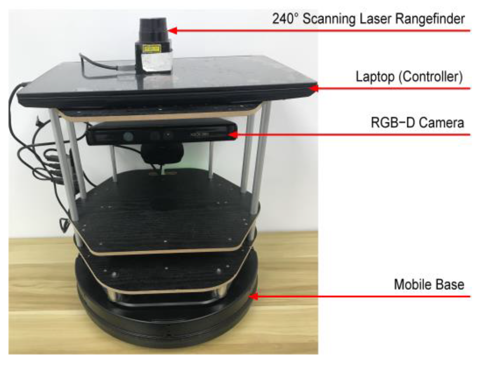
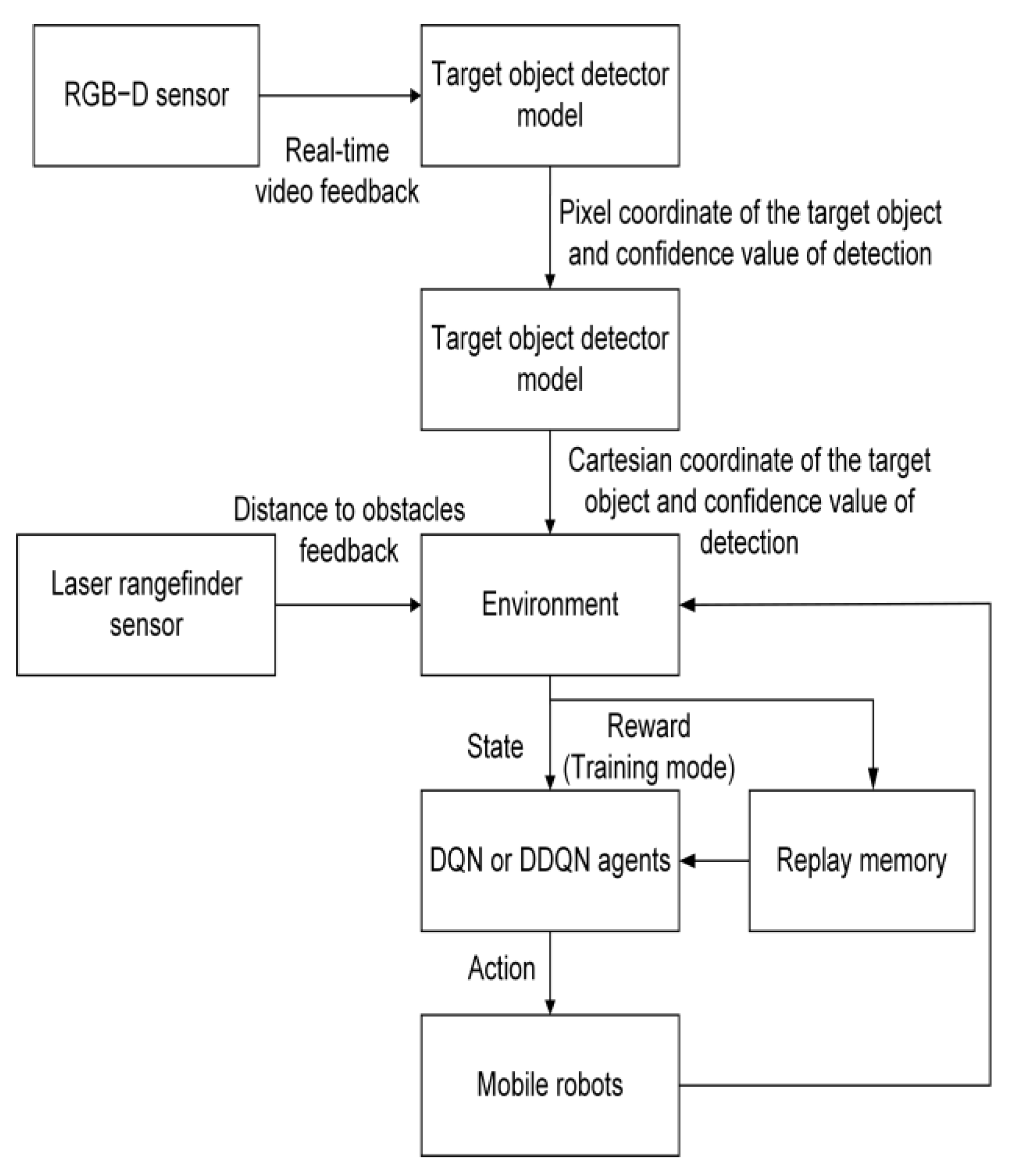
The proposed framework primarily consists of a mobile robot, an agent, and an environment. As shown in Figure 1, the mobile robot contains two sensors, such as a laser rangefinder and an RGB−D camera. The Hokuyo URG-04LX-UG01 with the following specifications 20 mm to 5600 mm detectable range, 240° area scanning range with 0.36° angular resolution, is used as a laser rangefinder sensor. This sensor uses a laser beam to determine the distance to an obstacle. It emits a laser pulse toward the obstacle and measures the flight time that the pulse reflected off the obstacle and returned to the laser rangefinder. The mobile robot can almost perceive its entire surroundings with its opening angle of 240°. It provides feedback to the mobile robot about the distance of the nearest obstacles. Microsoft XBOX 360 Kinect sensor with a 50 cm to 5 m range, 640 × 480 horizontal resolution, and about 1.5 mm at 50 cm and 5 cm at 5 m depth resolution is used as an RGB−D camera. An RGB−D camera has a horizontal opening angle of approximately 90°, which means only one-third of the field of view of the laser rangefinder is covered. However, it has a vertical opening angle of approximately 60°, which enables the 3D scan of the surroundings. An RGB−D sensor is used for feedbacking the real-time RGB and depth images of the surrounding environment to the mobile robot. The object detector model will take inputs from an RGB−D camera to search for the target object. Then, when the object detector model recognizes the target object, the mobile robot will start to navigate toward the target object. The proposed block diagram of autonomous mobile robot navigation in an unknown environment using a DQN or DDQN agent is shown in Figure 2.

An agent can be created with critic representation based on the state and action requirements of the environment using the following steps:

• Create state and action requirements for the environment.
• Specify the learning parameters of an agent.
• Create the agent using the DQN class of stable baselines.

Algorithm 1 shows the training of autonomous mobile robot navigation using DQL algorithms.

Algorithm 1 DQL Training
1:	Initialize the critic network with weights theta θ
2:	Initialize the target critic network with weights θ¯= θ
3:	Initialize replay memory D to capacity N
4:	For Episode = 1: K do
5:	Reset the environment
6:	Get the initial state Si of the environment
7:	Calculate the initial action Ai
8:	Set St and At to Si and Ai
9:	For Time-step t = 1: T do
10:	With probability ε select At for St
11:	Else, select At = argmaxa q (St, At; θ)
12:	Execute At
13:	Observe Rt+1, and St+1
14:	Store (St, At, Rt+1, St+1) in D
15:	Sample (St, At, Rt+1, St+1) from D
16:	If St+1 = ST, set qDQN (or qDDQN) to RT. Else, set
17:	qDQN (s, a)=Rt+1 + γmaxa′ (q′ (s′, a′; θ¯))
18:	qDDQN (s, a)=Rt+1 + γq′(s′, argmaxa′ q (s′, a′; θ); θ¯)
19:	Calculate L=1/M${\sum }_{i=1}^M$ (qDQN (or qDDQN) − q(s′, a′; θ))2
20:	Update θ
21:	Update θ¯ every 500 time-steps
22:	Update ε
23:	End For
24:	End For

3.3. Object Detector Model

The pre-trained deep learning, which is the Single Shot MultiBox Detector (SSD) MobileNet V2 model [45], is used for target object recognition. This model is the result of the combination of the SSD and MobileNets models. MobileNet is used for detecting the target object, while SSD is used for generating multiple bounding boxes. MobileNet is an object detector designed for mobile and embedded vision applications. MobileNet architecture uses depth-wise separable convolutions to build lightweight DNNs. The SSD architecture uses a single convolution network that learns to predict bounding box locations and classify these locations in a single pass, and it can be trained end-to-end. In this work, the object detector model is customized to focus on the detection and classification of the target object only (i.e., Coke can). An RGB−D camera provides a real-time video from which the object detector model continuously checks for the target object. Once the object detector model recognizes the target object from RGB−D videos, the mobile robot will start to navigate toward the target object.

3.4. DQL Agent Inputs and Outputs

Any RL-based agent takes state and reward as inputs and returns the action to be taken in the environment in each iteration. The state, action, and reward used for autonomous mobile robot navigation using DRL in unknown environments are described in detail as follows.

(1)

State: State is an observation of the environment that explains the current situation. For the agent, this is important because it would calculate and act depending on the state. The state size is 29, and 24 of them are laser distance sensor (LDS) values. The other five are the confidence of the detected target object, distances to the goal (target object location), angle to the goal (target object location), distance to the nearest obstacle, and angle to the nearest obstacle. The state is expressed as in Equation (7)

$$S=L_1+C_1+D_1+A_1+D_2+A_2,$$

(7)

where S: state; L₁: LDS (24 values); C₁: confidence of the detected target object (1 value); D₁: distance to the goal (1 value); A₁: angle to the goal (1 value); D₂: distance to the nearest obstacle (1 value); and A₂: angle to the nearest obstacle (1 value).

Initially, when the agent has no information on where the target object is in the environment (because the agent has not yet identified the target object in the environment), the following will take place. First, the target object detection confidence value of the SSD MobileNet V2 model is set to 0 (zero), the agent distance to the goal is set to the maximum possible value (5 m), and the agent angle to the goal is also set to 0 (zero). Next, once the target object is detected with a minimum confidence value (70%), the mobile robot will set the detected target object coordinate as the goal location and correspondingly updates the distance to the goal and angle to the goal values. Note that it is mandatory that the object detector model should increase its confidence value above the threshold confidence value (>85%) by the time the mobile robot reaches 1 m from the assumed goal location. The goal location is called “assumed” if the target object is detected with a minimum confidence value (70%). If the object detector model of the mobile robot fails to increase its confidence value above the threshold value by the time it reaches 1 m close to the assumed goal location, then the goal location is discarded, and the mobile robot will have to start searching for the new goal location. This set is used to avoid false predictions in the object detector model of the mobile robot. Finally, the mobile robot will navigate to the goal location.

(2)

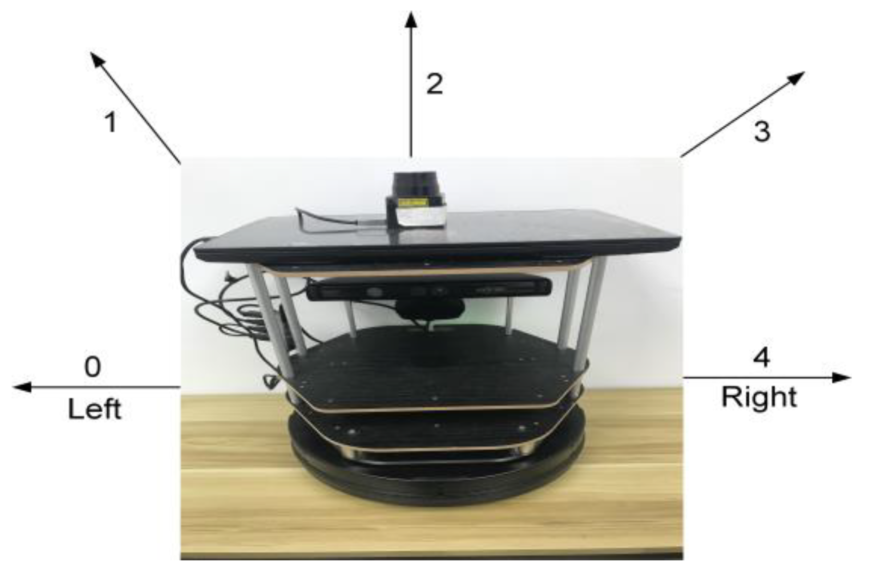
Action: Action is what an agent can do in each state. The mobile robot has five actions that it can act on depending on the type of state as shown in Figure 3. The mobile robot has a fixed linear velocity of 0.15 m/s and the angular velocity is determined by the action as shown in

Table 1. Action and angular velocity.

Action	Angular Velocity (rad/s)
0	−1.5
1	−0.75
2	0
3	0.75
4	1.5

. Initially, the agent knows nothing about the environment, so the agent cannot distinguish between the actions in the starting state in the first episodes. Thus, the trade-off between exploration and exploitation would be incorporated to address this issue. The trade-off between exploration and exploitation is a crucial feature of RL when an agent interacts with an environment. The justification for this feature of RL is that learning occurs online. Rather than working from a static dataset, the actions of the agent decide which data from the environment are returned. This implementation will allow us to consider not just how an agent performs its first actions, but how specifically it selects actions overall. The decisions taken by the agent decide the data it collects and thus, the data from which it can learn. The policy of our agent is a function that takes states and returns actions, and it can be expressed, as in Equation (8)

$$a=f(s),$$

(8)

where a: action; f: a function (i.e., DNN); and s: state.

Exploration is the process of discovering the environment to find information about it, whereas exploitation is the process of exploiting information that is already known about the environment to maximize the cumulative return. To balance exploitation and exploration, the “Linear Annealed Exploration” epsilon-greedy approach is used. In this approach, an exploration rate ε which is the probability of taking a random action is specified which is first set at 1. The probability that the agent would explore rather than exploit the environment at the start is called the exploration rate. It is 100% certain with ε = 1 that perhaps the agent will begin by exploring the environment. Linear annealed exploration starts with a high epsilon value (i.e., 1) and decrements a small amount of value linearly over each step of the time. After a set of time steps, the epsilon value remains at a fixed value (i.e., 0.02). This implementation ensures that at the beginning of the experiment, there is a lot of exploration and then it will exploit all the information at the end. This can be beneficial as the agent first has to explore the state space and then exploit the information after the agent has optimal actions. A linear annealed exploration is expressed, as in Equation (9)

$$\epsilon =\epsilon \times 0.1,$$

(9)

where ε: an exploration rate; 0.1: annealing factor.

(3)

Reward: Reward is a function that helps the agent to reach a conclusion rather than a prediction. A reward is a function that generates a scalar number representing a positive reward and a negative reward (penalty) for an agent for being in a particular state and taking a particular action. During training simulation, RL uses a reward generated by the environment to guide the learning process. This reward measures the agent’s performance with respect to the task objectives. In other words, the reward measures the efficiency of taking specific action for a given state. An agent updates its policy based on the rewards received for various state–action combinations. Generally, a positive reward is provided to encourage certain actions and a penalty to discourage other actions. The agent is guided by a well-designed reward to maximize the cumulative reward. However, the pre-trained weights are used for the agent during the testing simulation.

In the training simulation, at the starting state of the first episode in the training mode of simulation, the mobile robot and the target object location are set at (0, 0) and random location, respectively. The mobile robot will start searching for the target object by exploring the environment and it receives a reward of 0 before it identifies the target object. Once the target object is identified with a confidence value above the minimum confidence value, the DQL agent receives an immediate reward of 500. Then, the reward function (R_θ) for an angle can be derived from the angular direction in Figure 4 using Equation (11). The angular direction is used to show whether the mobile robot is facing directly toward the goal or not. For instance, if the robot is facing directly toward the target object (goal), then the angle is zero (θ = 0) and the action is equal to 2 (a = 2), if the robot is rotating in a clockwise direction from the goal, then the angle is varying from 0 to positive 180, and its action varies accordingly, and if the robot is rotating in a counter-clockwise direction from the goal, then the angle is also varying from 0 to negative 180, and its action varies accordingly. In Figure 4, the action block of lines indicates the action to be taken based on the angle from the robot to the goal. Equation (10) explains the angular direction of the robot from the goal, and Equation (11) explains the reward function from the angle. The reward from the angle is greater than or equal to 0 if the angle is between negative 90 and positive 90 degrees or less than 0 if the angle is not in the above-mentioned degrees. Likewise, the reward function (R_d) for the distance can be derived from the linear direction in Figure 5 using Equation (12). In Figure 5, the linear direction is used to show whether the robot is approaching the goal or not. If the robot is moving towards the goal, then the red strip line will move towards the left (origin), but if the robot is moving away from the goal, then the red strip line will move away from the origin. In Equation (12), if the current distance from the goal is less than the absolute distance from the goal, then the reward from the distance is greater than 2, but if the current distance from the goal is greater than or equal to the absolute distance from the goal then the reward from the distance is greater than 1 and less than or equal to 2. The reward function in Equation (13) is used for guiding the learning process of the DQL agent. Finally, the DQL agent receives a reward of 100, whenever the mobile robot gets closer to the (goal) target object location, and a penalty of −100 whenever the mobile robot moves farther away from the target object location or collides with obstacles.

$$\theta =\frac{\pi }{2}+a\times \frac{\pi }{8}+\varphi ,$$

(10)

$$R_{\theta }=5\times 1^{-\Lambda (\theta )}=\left\{\begin{array}{l}\ge 0,-\frac{1}{2}\pi <\theta <\frac{1}{2}\pi ,\\ <0,\mathrm{otherwise}.\end{array}\right.$$

(11)

$$R_d=2^{\frac{D_c}{D_g}}=\left\{\begin{array}{l}>2,D_c<D_g,\\ (1,2],\mathrm{otherwise}.\end{array}\right.$$

(12)

$$R=R_d\times R_{\theta }$$

(13)

where a: action; θ: angle from the mobile robot to the goal (target object); ϕ: yaw of the mobile robot; Λ: a function of an angle from the mobile robot to the goal; D_c: current distance from goal; D_g: absolute distance from goal; R_θ: reward from an angle; R_d: reward from a distance; and R: reward.

3.5. Mobile Robot Navigation Mechanism

The mobile robot receives inputs from the DQL agent, as well as the distance from obstacles using the laser rangefinder sensor, and also the current observations of the environment using an RGB−D camera. The output of the mobile robot is linear and angular velocities. The mobile robot’s autonomous navigation mechanism using a DQN or DDQN agent is outlined in detail as follows:

• The laser rangefinder feedback of the distance to the nearest obstacles for the mobile robot;
• An RGB−D camera feedback of the real-time video (color and depth images) of the current state of the environment for the mobile robot;
• The object detector model continuously checks for the target object in each frame of the video;
• The object detector model returns the confidence value of detection and the pixel coordinate of the target object when the target object is detected;
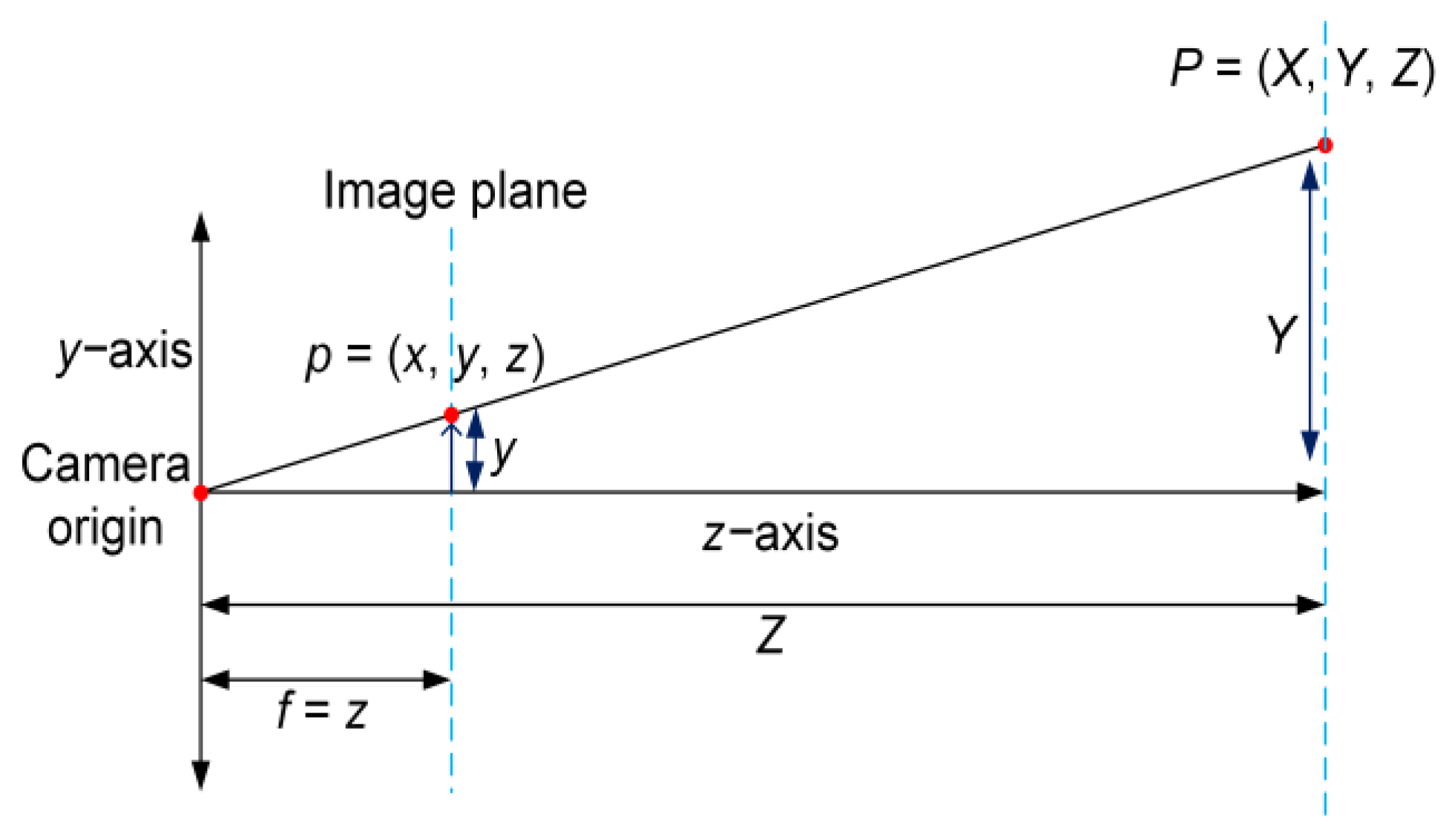
• The obtained pixel coordinate p = (x, y, z) of the target object is then projected into a real-world Cartesian coordinate P = (X, Y, Z) by using a similar triangle formula of the perspective imaging model that can be expressed as in Equations (14)–(16). Where depth (d) is the distance from an RGB−D camera to the target object and it is obtained from the depth image (assuming that an RGB−D camera is pointing along the positive z-axis and the x-axis is equal to 0), and f is the focal length of the lens, as shown in Figure 6;

$$X=d\times \frac{x}{z},$$

(14)

$$Y=d\times \frac{y}{z},$$

(15)

$$Z=d,$$

(16)

6.

The real-world Cartesian coordinates of the target object that are obtained with respect to an RGB−D camera are transformed to the origin of the mobile robot using the ROS tf package (transformation from an RGB−D camera coordinate frame to the mobile robot origin coordinate);

7.

Finally, the mobile robot starts to navigate to the target object based on the state received from the laser rangefinder sensor and an RGB−D camera.

3.6. Stable Baselines

The control system scheme for the proposed autonomous navigation of mobile robots in an unknown environment is a DRL. Therefore, the control system problem has been identified as an instance of DRL. Ideally, one might want to apply a DQL algorithm to learn the optimal performance. Stable baselines [46] is the most commonly used instantiation of the DQL algorithm. It is a set of improved implementations of RL algorithms that is a clone of an OpenAI Baselines [47] library, which uses the TensorFlow framework to create the DNN used to estimate the Q-function. Hence, the DQN class of the stable baselines with its extension such as DDQN is used for creating the DNN to estimate the Q-function. The DRL algorithms used for the autonomous navigation of mobile robots have been built on the top of the DQN class of the stable baselines, which is a very simple and efficient way to build the DRL agents. To use the DQN class of the stable baselines, it is first necessary to inherit an OpenAI Gym, which is used to interface the DQN class with its working environments. Next, the ROS Kinetic uses Python 2, whereas stable baselines and OpenAI Gym use Python 3, so to bridge this gap a socket communication was established between the Gym environment and the ROS-based Gazebo environment. Finally, the DQN class is connected with ROS and Gazebo for behavior learning of autonomous mobile robot navigation. The default option of the DQN class, which is a multilayer perceptron (MLP) with 2 hidden layers of 64 nodes, is used for estimating the Q-function.

Table 2. Experimental parameters for DQN and DDQN agents.

Parameter	Value
Discount factor	0.99
Buffer size	1,000,000
Batch size	64
Number of training time steps	150,000
Learning rate	5 × 10−4
Initial epsilon	1
Final epsilon	0.02
Target network update frequency	500
Epsilon annealing factor	0.1

shows the experimental hyperparameters used for training the DQN and DDQN agents.

4. Results

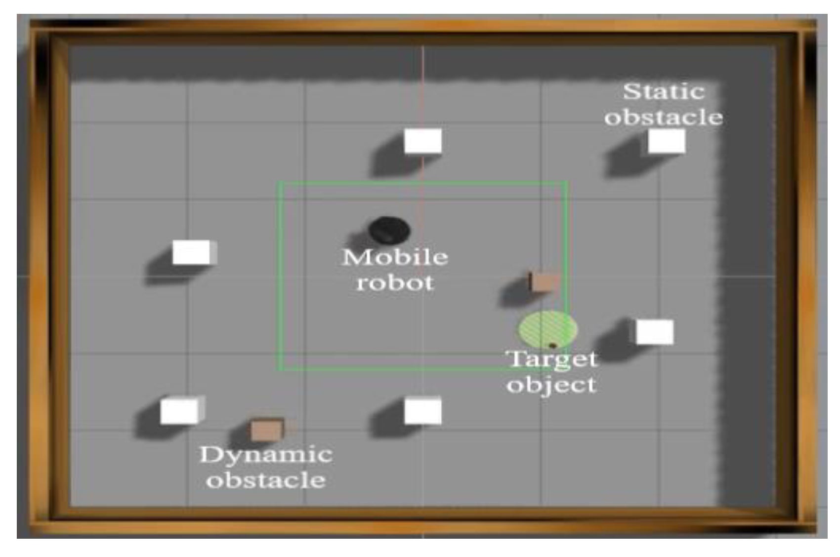
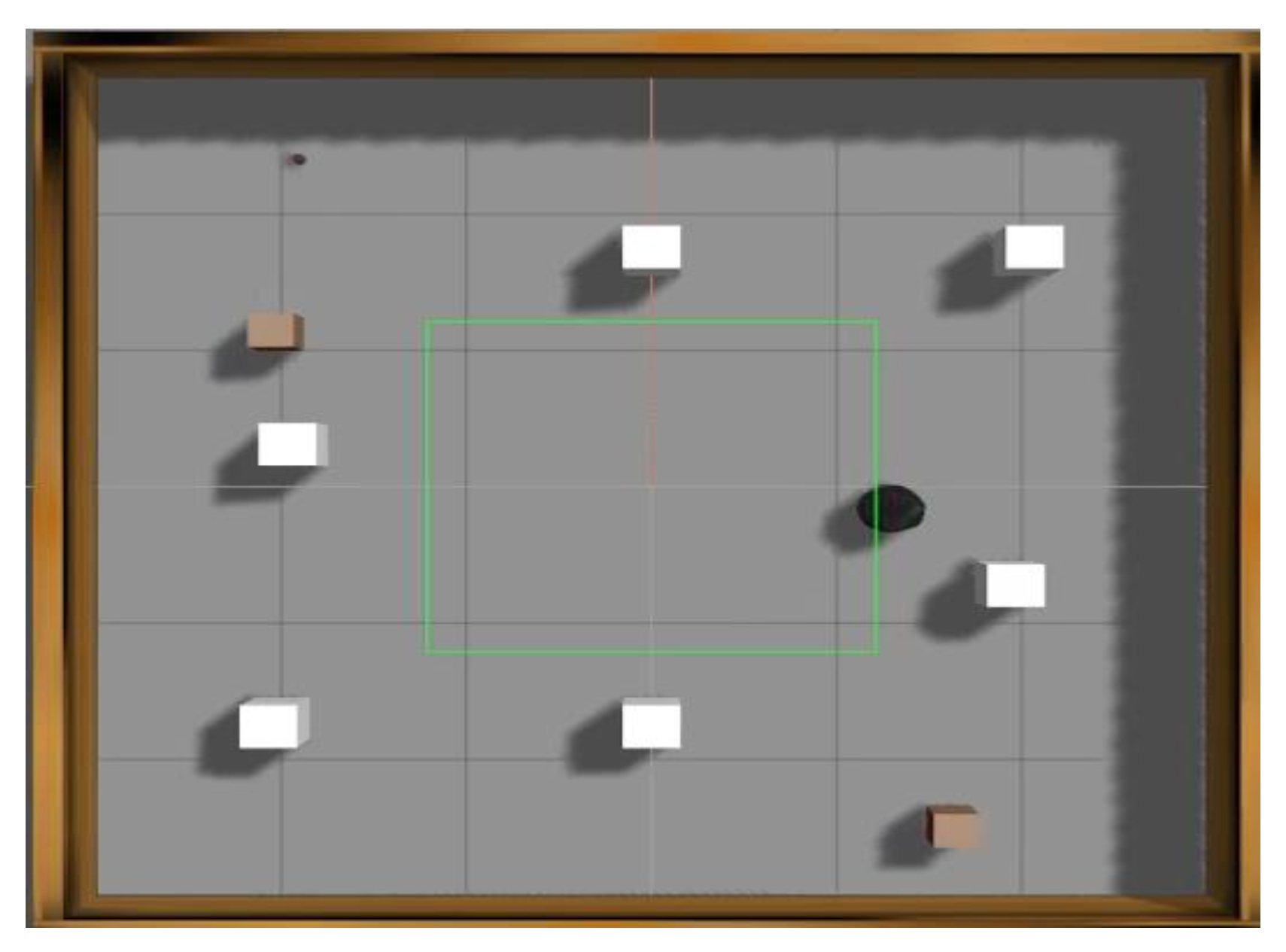
The proposed algorithms for the autonomous navigation of mobile robots in an unknown indoor environment built in the Gazebo simulator are evaluated in this section. The target object recognition experiment was first conducted without any obstacles to verify that the object detector model operates in real time. 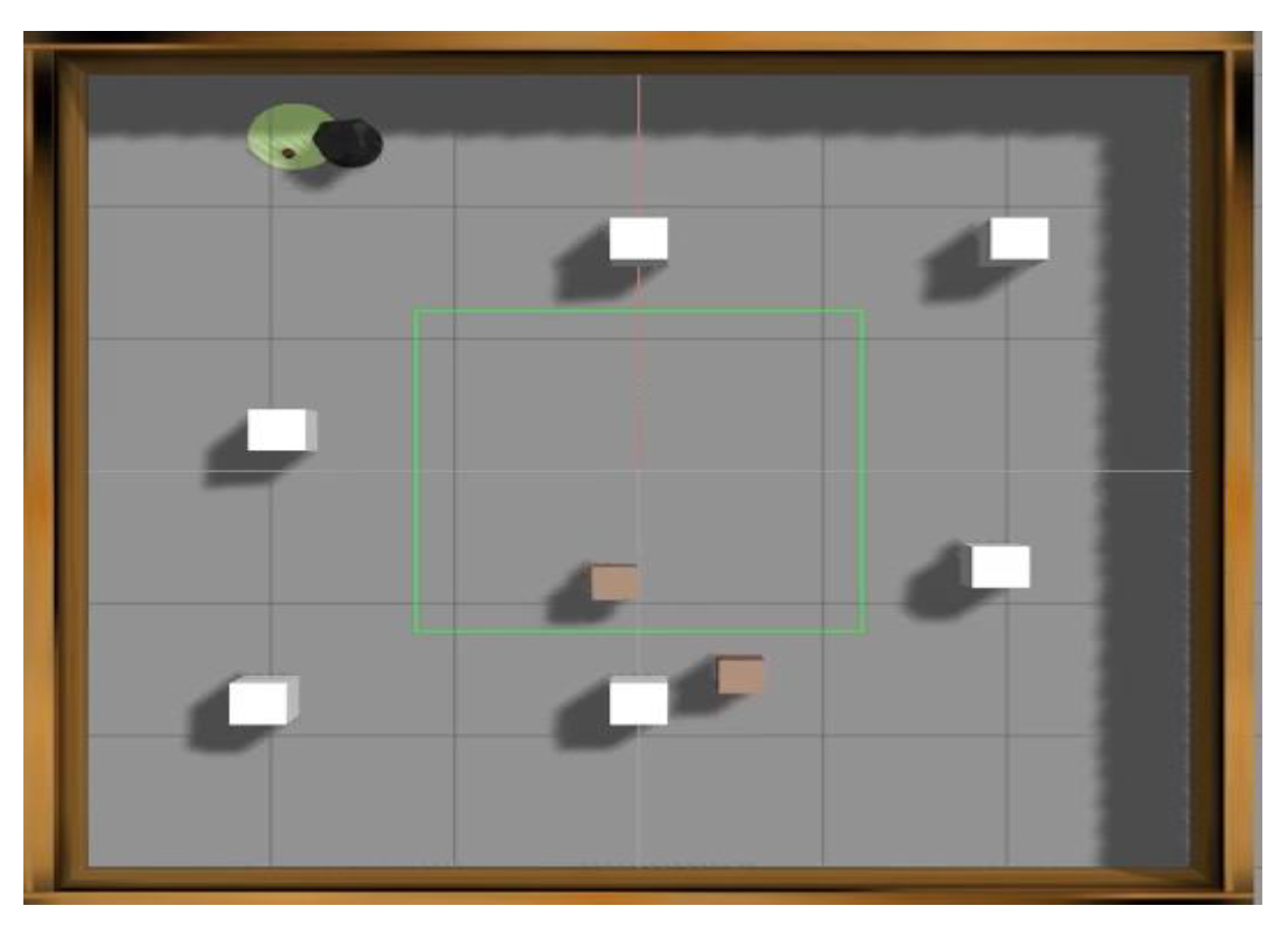Then, the proposed DQN agent’s capability of autonomous navigation is evaluated in an indoor environment of “6 m × 6 m,” with both static and dynamic obstacles, as shown in Figure 7. In the Gazebo simulation environment, the following things will take place for DQN agent learning. First, the mobile robot will search for the target object by exploring the environment. Next, once the mobile robot discovers the target object, the target object will be labeled with a yellow marker to indicate that it is the goal location. 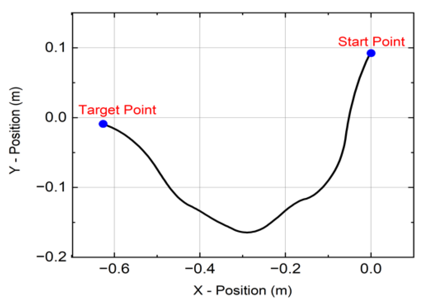Finally, the mobile robot will navigate to the goal location as shown in Figure 8 and Figure 9, respectively, for the DQN agent. 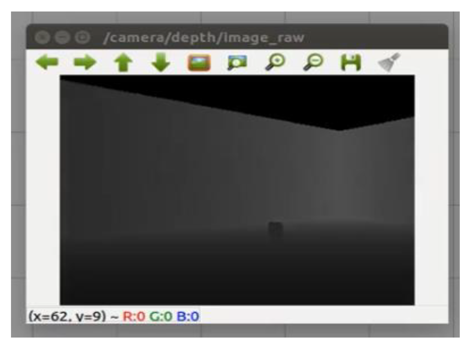The trajectory of the mobile robot from the random starting location to the target location using the DQN agent is shown in Figure 10. The mobile robot has an RGB−D camera which is used to collect real-time RGB and depth images simultaneously from the state of the environment. Figure 11 shows the depth image of the target object from an RGB−D camera. Similarly, the DDQN agent capability of autonomous navigation is evaluated in the same environment. In the training simulation, the simulation experiment completes after 150,000 time-step limits are exceeded. 150,000 time steps is the maximum number of time steps that the DQN and DDQN agents take before the simulation experiment auto-terminates. This time step is selected initially by default to train a DQN agent. The training took around 15 h, so this time step is used for all discount factors as well as a DDQN agent. However, in each episode, if the mobile robot either collides with an obstacle or does not reach the target object location within 100 time-step limits, then, the current episode will auto-terminate. In other words, a new episode will start if the mobile robot either collides with an obstacle or reaches 100 time-step limits, and the mobile robot will start from the origin (0, 0) in each new episode. However, the mobile robot will continue from the last state of the previous episode if the mobile robot reaches the target object’s location. A maximum number of 100 time steps is used in each episode to prevent over-fitting of the agent’s models. Note that the proposed method is implemented in Python 3.6 with TensorFlow 1.14.0 and 1.13.2 for target object recognition and autonomous navigation of mobile robots using DRL agent, respectively, with an Intel Core i7-9750H central processing unit (CPU) and GeForce GTX 1650 graphical processing unit (GPU) with a Max-Q design.

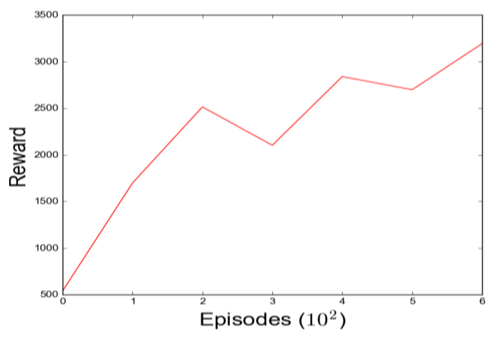
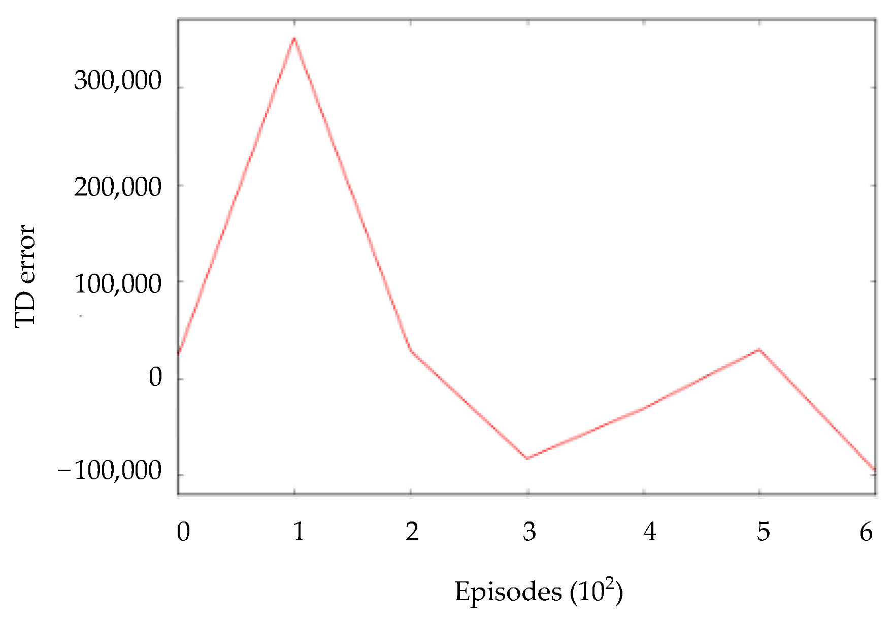
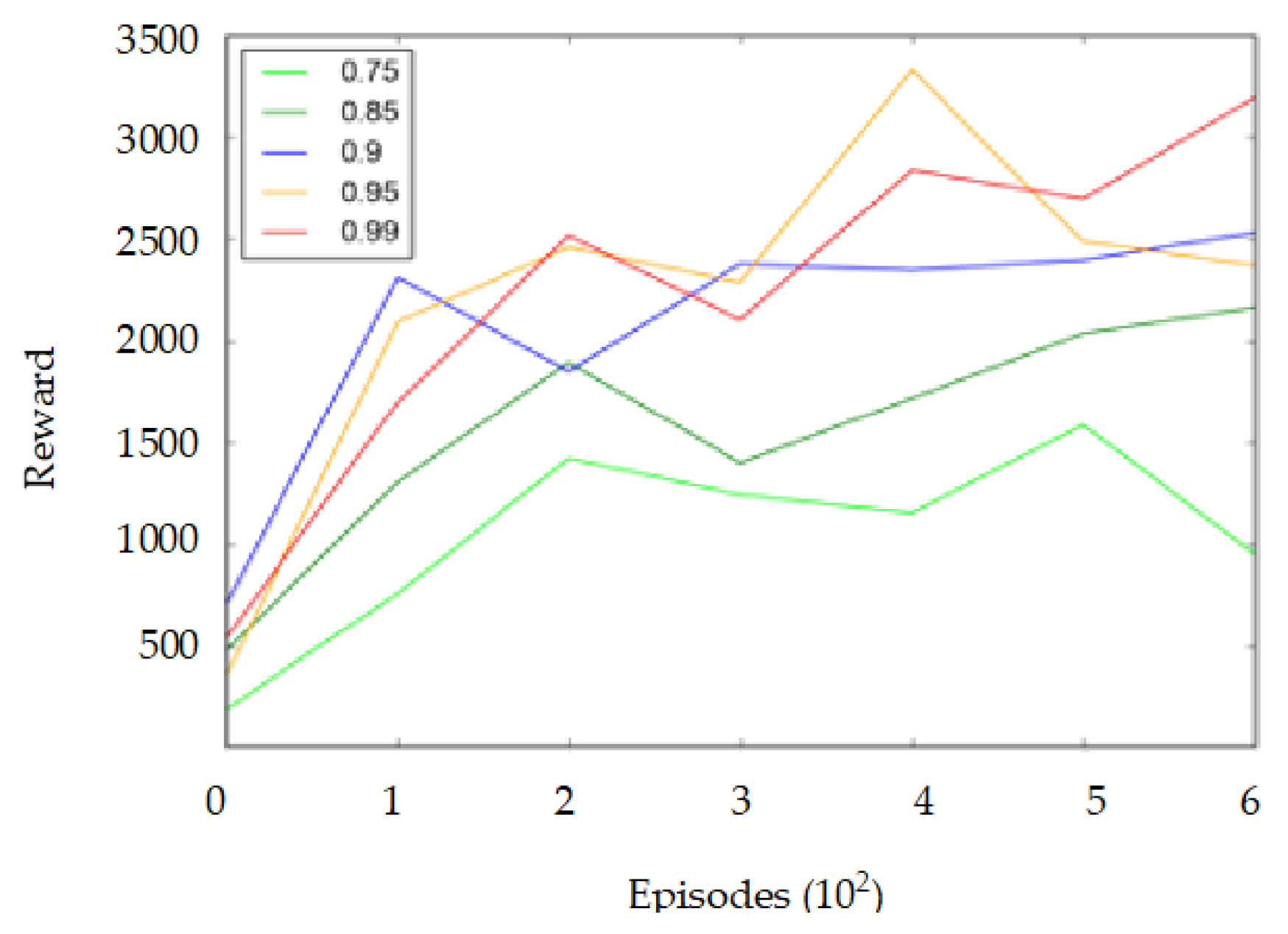
The average cumulative reward over 100 batch size received by a DQN agent in the Gazebo simulator after training the mobile robot for 150,000 time steps is shown in Figure 12. The average cumulative TD error over 100 batch size of a DQN agent in the Gazebo simulator after training the mobile robot for 150,000 time steps is shown in Figure 13. 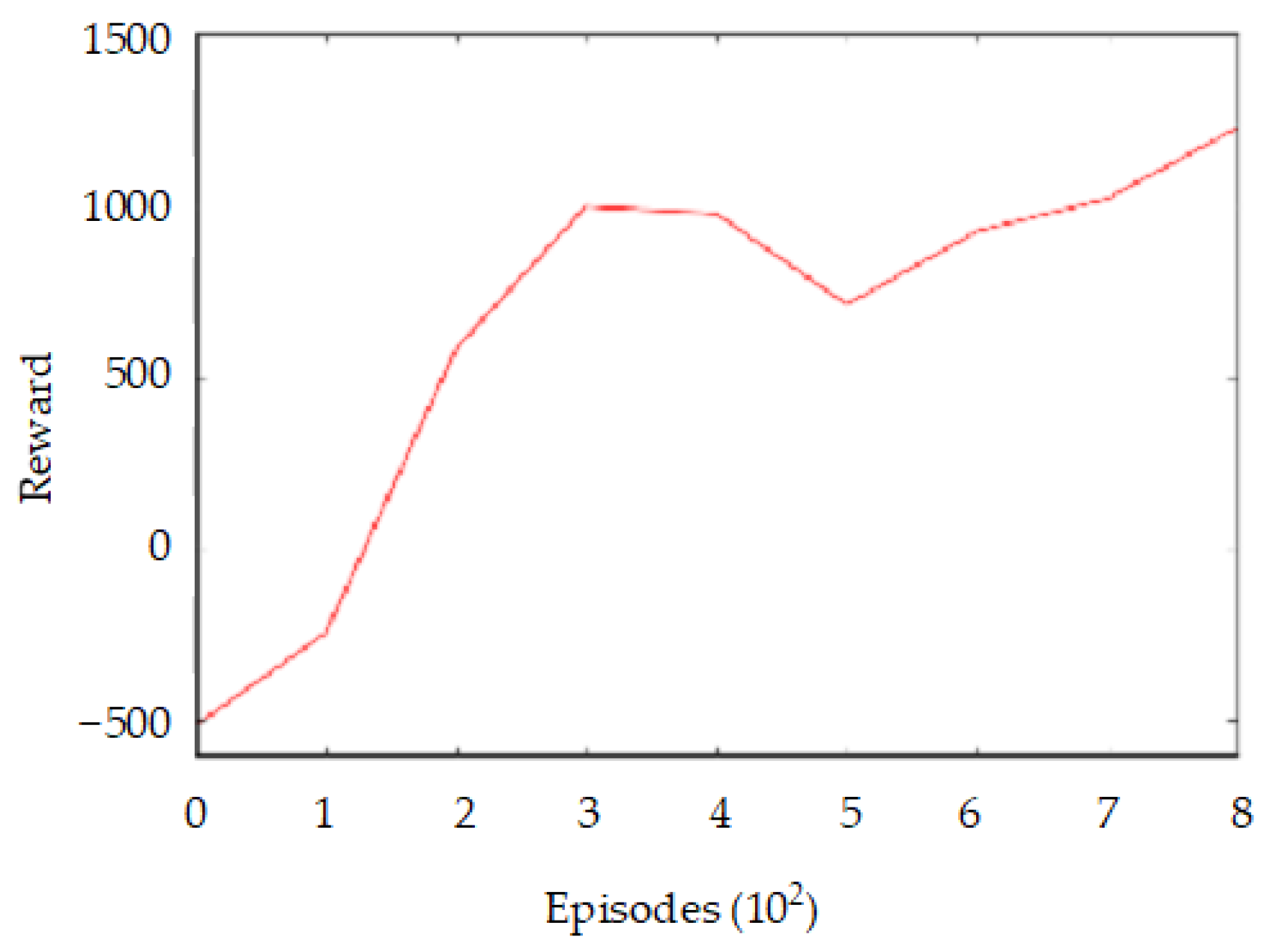The average cumulative reward over 100 batch size received by a DQN agent in the Gazebo simulator after training the mobile robot for 150,000 time steps for different discount factor values is shown in Figure 14. The average cumulative reward over 100 batch size received by a DDQN agent in the Gazebo simulator after training the mobile robot for 150,000 time steps is shown in Figure 15. The average cumulative TD error over 100 batch size of a DDQN agent in the Gazebo simulator after training the mobile robot for 150,000 time steps is shown in Figure 16. Finally, the average cumulative reward over 100 batch size received by a DDQN agent in the Gazebo simulator after training the mobile robot for 150,000 time steps for different discount factor values is shown in Figure 17.

Real-World Results

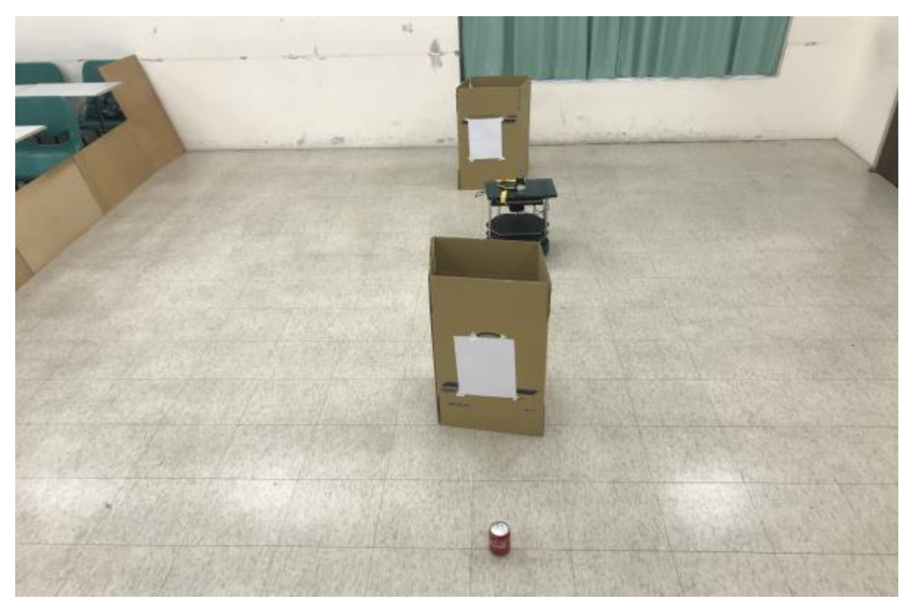
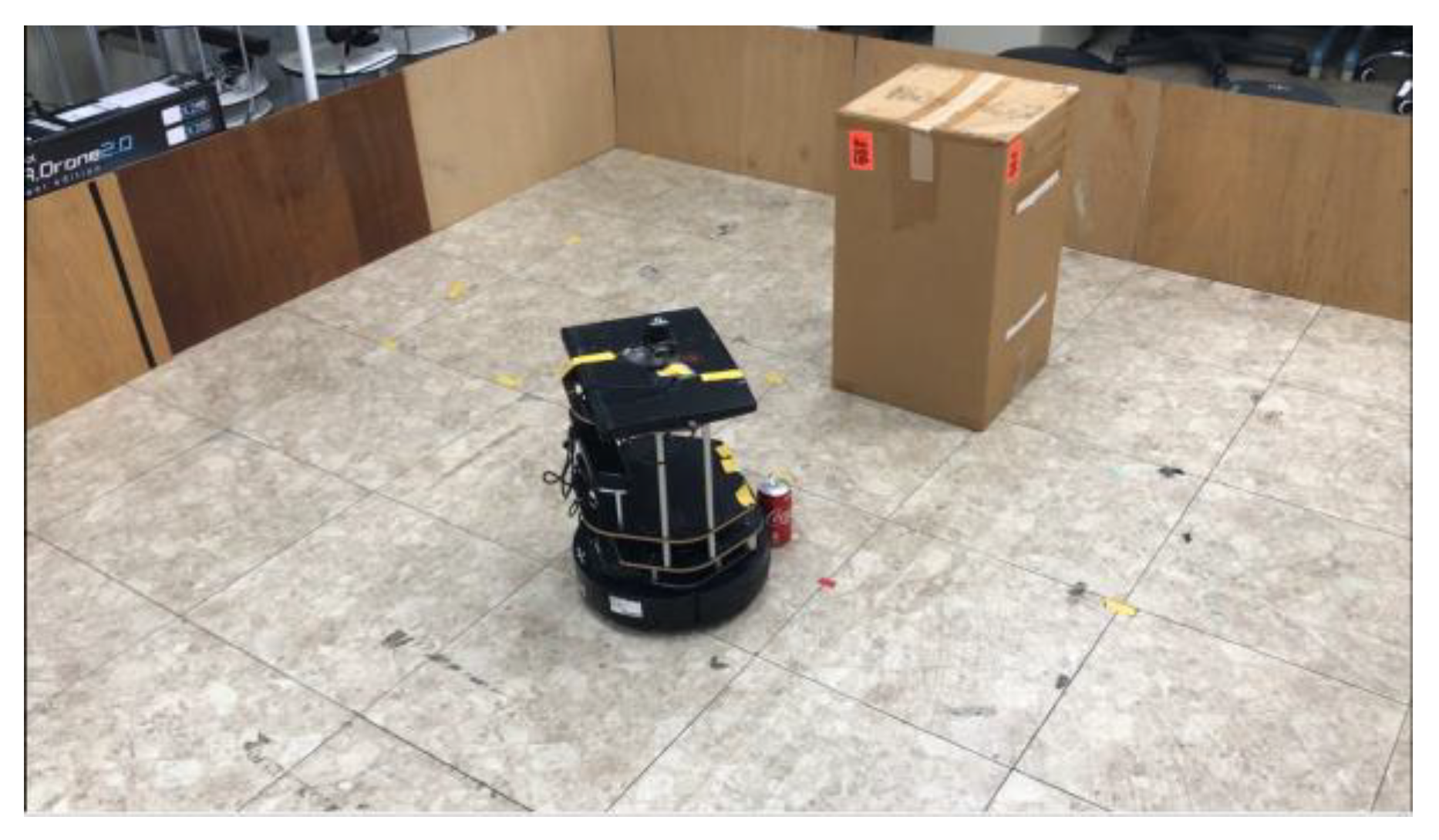
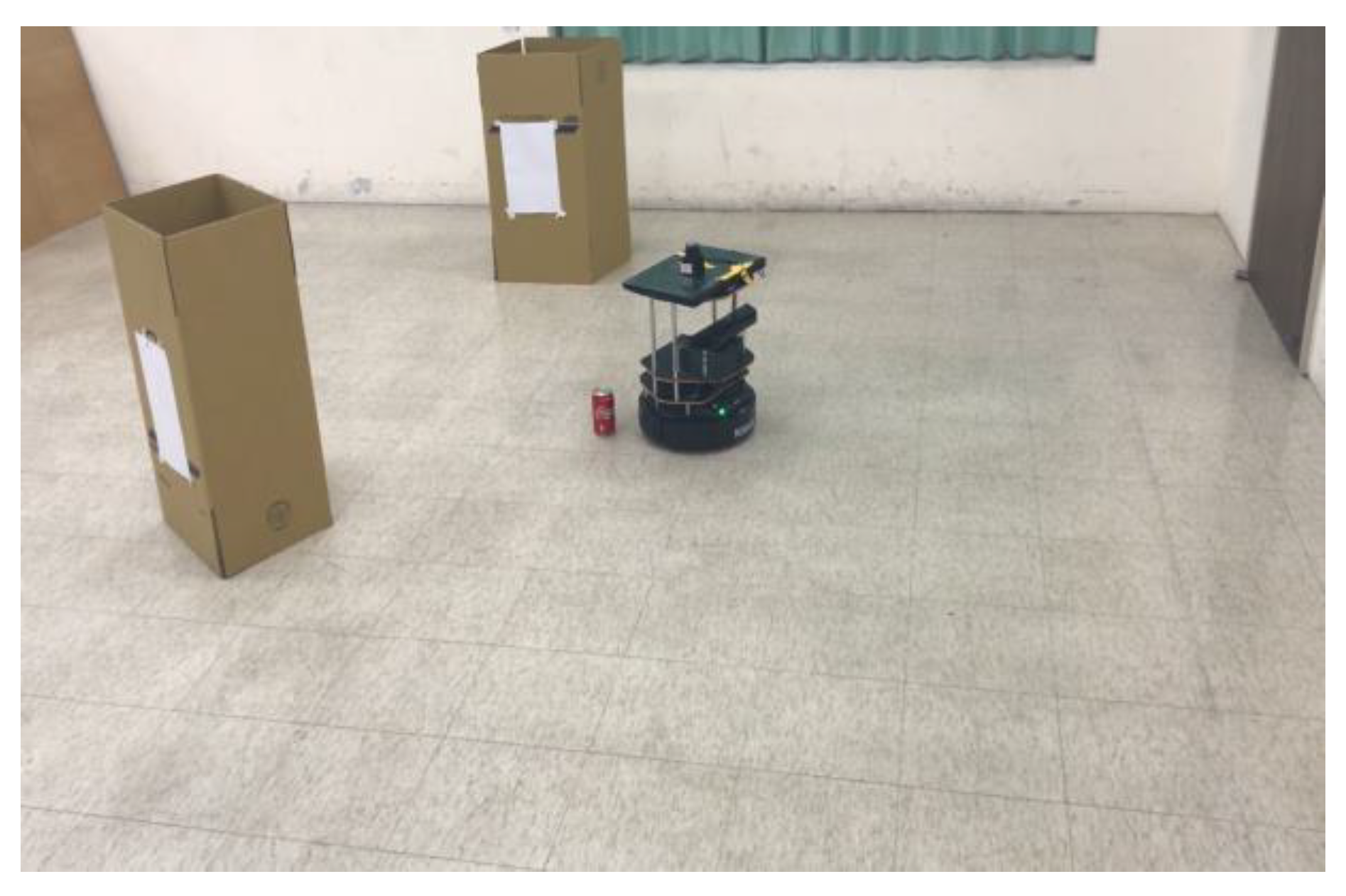
The proposed DQL algorithm for the autonomous mobile robot navigation problem in real unknown indoor environments is evaluated. The mobile robot consists of two sensors: an RGB−D camera and a laser rangefinder sensor. The mobile robot is operated directly from a laptop (controller) using the Ubuntu 16.04 system, and another second laptop is used to remotely control the laptop on the mobile robot using Zoho Assist software. Zoho Assist software is a cloud-based remote support and access software that allows one to remotely control another computer. The DQL agent directly controls the mobile robot from a laptop. The trained DDQN policy is first evaluated in an indoor environment of “4 m × 3 m”, with one static obstacle and the target object. Next, it is evaluated in an indoor environment of “5.1 m × 4.7 m”, with two static obstacles and the target object. The real-world arena used for evaluating the mobile robot’s autonomous navigation is shown in Figure 18 and Figure 19, respectively. First, the mobile robot will search for the target object by exploring the environment starting from its initial location. Then, once the target object is recognized, the mobile robot will navigate to the target object’s location as shown in Figure 20 and Figure 21, respectively.

5. Discussion

In the average cumulative reward per episode of a DQN and DDQN agent as shown in Figure 12 and Figure 15, respectively, it can be noticed that in the first episodes the average cumulative reward of the DDQN agent is negative but not for the DQN agent. A DDQN agent takes a longer time and more episodes to achieve a high cumulative reward, while a DQN agent takes less time and fewer episodes to even achieve a high cumulative reward. However, the DDQN agent’s cumulative reward is more consistent than the DQN agent’s. The average cumulative TD error of the DQN and DDQN agents as shown in Figure 13 and Figure 16, respectively, are decrementing with episodes, which indicates that the error difference between the target critic and the critic networks of DQN and DDQN agents are reducing. The average cumulative reward received by the DQN and DDQN agents in the Gazebo simulator after training 150,000 time steps for different discount factor values is shown in Figure 14 and Figure 17. Thus, from Figure 14 and Figure 17, it can be observed that a 0.99 discount factor value is the best for obtaining the highest average cumulative reward per episode for both agents during the training mode. Hence, a 0.99 discount factor value for training and evaluating the DQN and DDQN agents is used. In the training simulation environment, the agent learned policies to navigate autonomously while avoiding dynamic and static obstacles.

The same protocol is followed during the test mode in the Gazebo simulation except that the learned policies are used for the autonomous navigation of mobile robots. In test mode, the simulation experiment is only conducted for 100 episodes. Since the proposed method is end-to-end, the learned policies are deployed to the real mobile robot for autonomous navigation of mobile robots in an unknown indoor environment. The simulation results of the DQN and DDQN agent’s comparison, which are both trained for the same number of training time steps in the Gazebo simulator, are evaluated five times in the test simulation of the Gazebo simulator each for 100 episodes. The DQN and DDQN agents’ mean, sample standard deviation, and max number of goals are compared as shown in

Table 3. DQN and DDQN agents’ comparison.

No. of Goals	DQN	DDQN
Mean	150	158
Sample standard deviation	11.22	10.88
Max	163	171

Note: the results shown in Table 3 are not always constant, which means that the results may be different for the new test simulation in the Gazebo simulator.

. The DDQN agent outperforms the DQN agent by 5.06% in reaching the location of the target object overall because the DDQN agent reduces overestimation in the value function estimation. Hence, for verifying the mobile robot’s autonomous navigation in the real-world experiment, only the DDQN agent is used.

Finally, the proposed DDQN agent’s autonomous navigation capabilities are evaluated in two different real-world indoor environments. First, the autonomous navigation capability of the DDQN policy is evaluated in the area of “4 m × 3 m” with one static obstacle and the target object. Next, the DDQN agent capability of autonomous navigation is evaluated in the area of “5.1 m × 4.7 m” with two static obstacles and the target object. Since the proposed approach is an end-to-end approach, the algorithm used in the test mode simulation is not modified (fine-tuning) during deployment to the real mobile robot. The real-world environment is completely different from the simulation environment in terms of area dimension and number of obstacles, yet the proposed algorithm can work decently. An improvement in [28] is made by deploying the algorithm to the real mobile robot. The real mobile robot is able to search for the target object by exploring the environment. Once the target object is recognized by the object detector model, the mobile robot will be able to navigate to the target object’s location by avoiding static obstacles as shown in Figure 20 and Figure 21. Thus, DQL agents have been successfully built, trained, and evaluated for autonomous mobile robot navigation in both simulation and real-world environments. Where both static and dynamic obstacles are used in the simulation environments, however, in the real-world environments only static obstacles are used.

6. Conclusions

Mobile robot autonomous navigation in unknown indoor environments using DRL algorithms was presented and evaluated. The proposed DQL algorithms are so powerful that there is no need for agents to know anything about the environment since they can still learn how to interact with the environment. The agents can work with any kind of mobile robot without requiring the kinematics and dynamics of the mobile robot because the proposed algorithms are model free. The simulation results show that the proposed autonomous navigation algorithms would allow the mobile robot to navigate autonomously and free of collisions to the target object location in both static and dynamic obstacles without the prior development of an environmental map. The object detector model would enable the mobile robot to recognize the target object in real time.

A practical approach is proposed for collision avoidance and goal-oriented navigation tasks of mobile robots using DQN and DDQN agents. From the experiment, it has been seen that the DQN and DDQN agents trained in the Gazebo simulator can be deployed directly to the real mobile robot without tuning the parameters. The DDQN agent is more robust and better than the DQN agent in exploring the environment, avoiding collisions, and reaching the target object location from the simulation experiment in Gazebo. Thus, only the DDQN agent is used for real-world experiments in an unknown indoor environment. The real-world experiment is performed in two different environments to demonstrate that the deployed DDQN policy without a learning algorithm is capable of operating in the real world. In conclusion, the proposed method has great potential for autonomous mobile robot navigation compared with SLAM, however, the reward design is the challenging part of DRL for autonomous mobile robot navigation. In the real-world experiment, the final model configuration will have a single board computer (NVIDIA Jetson TX2), which has excellent processing speed with a hex-core CPU, a 256-core NVIDIA pascal GPU, and 8G LPDDR4 RAM, instead of a laptop as a controller unit.

In the future, a new reward function will be proposed to facilitate the evolution of different behaviors including: adding new features to the environment; deploying both the policy and the learning algorithm on the real mobile robot so that the agent continues to learn to obtain optimum performance in the real world after deployment; making the environment of real-world experiments identical to the Gazebo simulation experiment environment; designing a Deep Deterministic Policy Gradient Agents (DDPG) algorithm to get continuous action space to ensure smooth and continuous motion of the mobile robot; and designing the backend of a DRL algorithm from scratch (not using the DQN class of the stable baselines) to access all the callbacks such as loss, average max Q-value, and cumulative max Q-value.