A Computational Framework for Design and Optimization of Risk-Based Soil and Groundwater Remediation Strategies

Highlights

What are the main findings?

• A computational framework is developed for design of soil and groundwater remediation strategies.
• Machine-learning and process-based models are integrated to expedite computation in the framework.

What is the implication of the main finding?

• The applicability of the framework is successfully demonstrated at a field site contaminated with arsenic.

Abstract

Soil and groundwater systems have natural attenuation potential to degrade or detoxify contaminants due to biogeochemical processes. However, such potential is rarely incorporated into active remediation strategies, leading to over-remediation at many remediation sites. Here, we propose a framework for designing and searching optimal remediation strategies that fully consider the combined effects of active remediation strategies and natural attenuation potentials. The framework integrates machine-learning and process-based models for expediting the optimization process with its applicability demonstrated at a field site contaminated with arsenic (As). The process-based model was employed in the framework to simulate the evolution of As concentrations by integrating geochemical and biogeochemical processes in soil and groundwater systems under various scenarios of remedial activities. The simulation results of As concentration evolution, remedial activities, and associated remediation costs were used to train a machine learning model, random forest regression, with a goal to establish a relationship between the remediation inputs, outcomes, and associated cost. The relationship was then used to search for optimal (low cost) remedial strategies that meet remediation constraints. The strategy was successfully applied at the field site, and the framework provides an effective way to search for optimal remediation strategies at other remediation sites.

1. Introduction

Soil and groundwater contamination is still a major environmental problem in many countries. According to European Environment Agency, soil contaminants exist in almost 250,000 sites in Europe, where heavy metals and metalloids are the most common contaminants [1]. In China, a survey found that 16.1% of soil locations exceeded the regulatory control levels with the average contents of cadmium (Cd), arsenic (As), and mercury (Hg) exceeded the regulatory control levels by 7.0%, 2.7%, and 1.6%, respectively [2]. Various active remediation technologies have been developed and used to restore the contaminated soils in the contaminated sites. These technologies include soil replacement [3], stabilization/solidification [4], soil washing [5], and thermal remediation [6]. However, most of the active remediation technologies do not consider the natural attenuation potential in soil and groundwater environment, often leading to over-remediation and a significant cost burden [7,8]. Remediation technologies that can fully consider the combined effects of active remediation and natural attenuation are needed to significantly reduce remediation cost. Remediation cost is a major factor in assessing the feasibility of remediation strategies, especially in regions with the constraints of financial resources.

The geochemical and biogeochemical processes in soil and groundwater systems can degrade or attenuate contaminants. Contaminants can undergo dilution, dispersion, sorption, redox transformation, and degradation that may reduce their concentrations or toxicity to acceptable levels. Monitored natural attenuation (MNA) is a type of remediation technology that takes advantage of the geochemical and biogeochemical processes to treat contaminants in soil and groundwater systems with significant cost saving [9,10]. The challenge for applying MNA technologies is that it usually takes a long time [11,12]. For the contaminated lands with plans for near-future re-development, MNA will be difficult to meet the time constraint. Under such scenarios, active remediation technologies are often implemented without considering the natural attenuation potentials. The trade-off is the significant increase of remediation cost.

In this study, a numerical framework was developed that can fully consider the effects of active remediation technologies and natural attenuation in designing remediation strategies. The geochemical and biogeochemical processes were integrated using process-based models, which were used to simulate the effects of various remediation strategies with integrated active remediation technologies and natural attenuation on residual concentrations and distributions of contaminants in soil and groundwater systems. Extensive simulations were, however, required to find an optimal strategy that can minimize the cost of the remediation and meanwhile meet remediation requirements. To reduce the computational burden, selective simulations of remediation strategies were performed and the simulated results were used to train a machine learning (ML) model, random forest regression (RFR), with a goal to establish the relationships between the outcomes and costs of remediation strategies. The trained RFR was then used to search for an optimal remediation strategy within the constraints of the remediation requirements using a global optimization method. The approach was successfully demonstrated at a remediation site contaminated with As and can be applied at other contaminated sites for designing and optimizing remediation strategies.

2. Methods

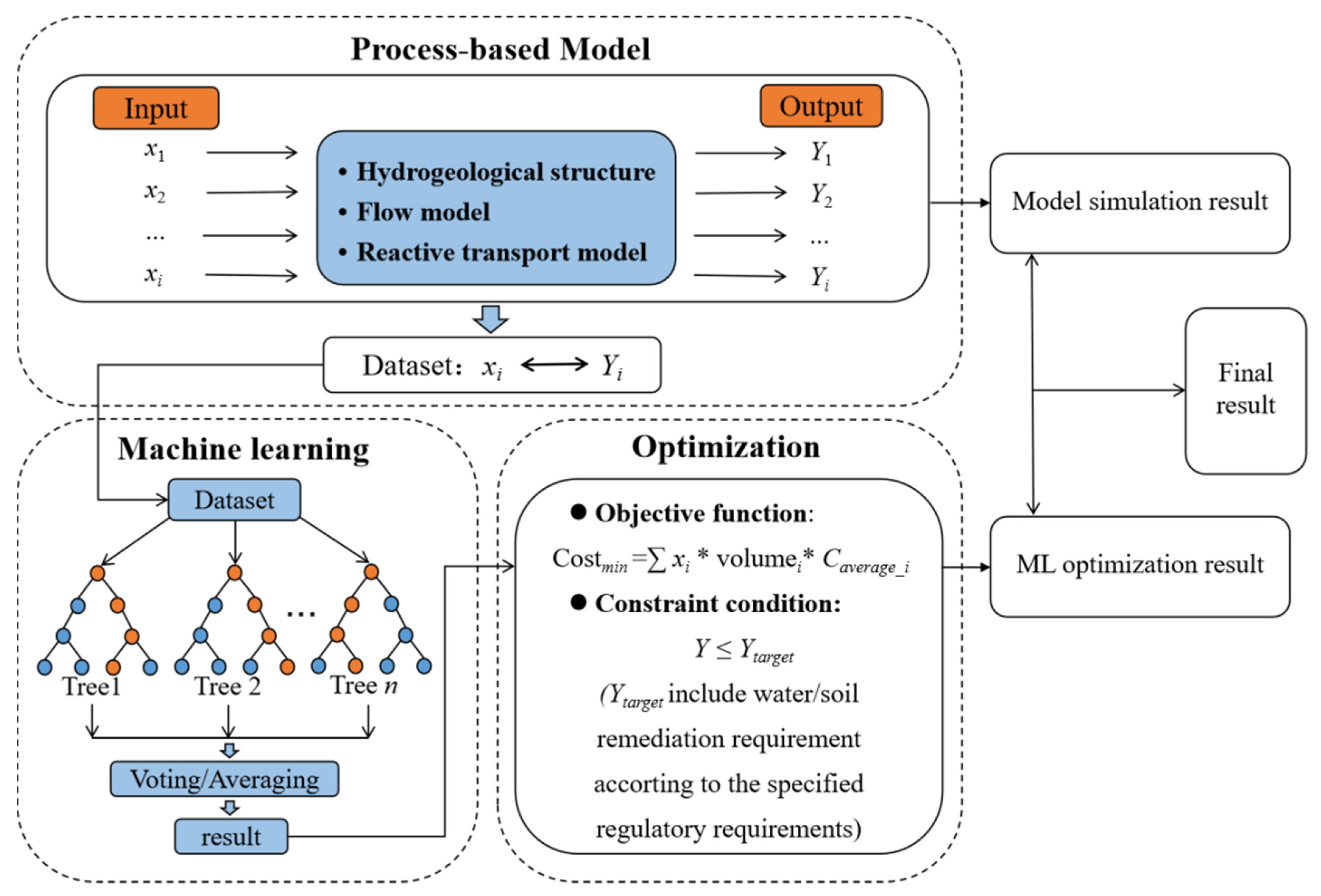
2.1. Model Framework

The model framework for designing remediation strategies at a target site consists of a process-based simulation module, ML module, and optimization module (Figure 1). The process-based module was used to simulate reactive transport of contaminants under natural and remedial conditions to obtain various types of simulated data such as spatial and temporal changes of contaminant concentrations, contaminant migration paths and discharges to nearby sensitive locations such as river, and remediation costs for different remedial strategies. The obtained data were used to train an ML model in the ML module to establish the relationship between input and output variables in a target remediation site. In this study, the input variables (xi in Figure 1) are those related to hydrological and biogeochemical boundary and initial conditions, as well as those related to remedial activities, such as a set of remediation strategies to be adopted at the site, the locations and extents for each adopted technology, the locations and amounts of injecting reagents, etc. The output variables (Yi in Figure 1) are the simulated outcomes obtained from the process-based model, such as residual contaminant concentrations and their spatiotemporal distributions in groundwater and soil, contaminant flux and its spatiotemporal distributions, etc. These variables were used in both the process-based and ML modules. The trained ML model was then used by the optimization module to find a suite of optimal strategies that meet the remediation requirements for site decision makers to select a final strategy to be implemented. In the framework, the remediation requirements are often the time constraints and the regulatory control levels. For example, for a site contaminated with As, the remediation requirement for groundwater concentration is <10 ug/L.

2.1.1. Process-Based Simulation Module

PFLOTRAN, an open-source, massively parallel simulator of subsurface flow and reactive transport [13,14] was used in this study to simulate contaminant transport under both natural and remedial conditions. The simulator solves Richards equation for subsurface flow [15].

$$\frac{\partial }{\partial t}\left(ns\rho \right)+\nabla ·\left(\rho q\right)={\mathsf{\Omega }}_{\omega }$$

(1)

$$q=-\frac{k{k}_r\left(s\right)}{u}\left(\nabla P-W_w\rho gz\right)$$

(2)

where n is the porosity (−), s is the saturation degree (m³/m³), ρ is the water density (kmol/m³), q is the Darcy velocity (m/s), k is the intrinsic permeability (m²), k_r is the relative permeability (−), μ is the viscosity (Pa∙s), P is the pressure (Pa), W_w is the molecular weight of water (kg/kmol), g is the gravity (m/s²), and z is the vertical component of the position vector (m). Water density and viscosity are functions of temperature and pressure. The source/sink term Ω_ω (kmol/m³∙s) has the form:

$${\mathsf{\Omega }}_{\omega }=\frac{qM}{W_{\omega }}\delta \left(r-r_{ss}\right)$$

(3)

where qM denotes a mass rate in kg/m³/s, and r_ss denotes the location of the source/sink.

The solute reactive transport in the model was simulated using the following equations [13]:

$$\frac{\partial }{\partial t}\left(n{\displaystyle \sum }_{\alpha }s{C}_j^{\alpha }\right)+\nabla ·{\displaystyle \sum }_{\alpha }{Q}_j^{\alpha }=-{\displaystyle \sum }_m{v}_{jm}{R}_m$$

(4)

for the jth primary species, and

$$\frac{\partial {\theta }_m}{\partial t}=\overline{V_m}{R}_m$$

(5)

for the mth mineral. In Equations (3) and (4), $C_j^{\alpha }$ and $Q_j^{\alpha }$ denote the total concentration and flux, respectively. The R_m is the reaction rate, v_jm is the reaction stoichiometric coefficients, ${\theta }_m$ is the mineral volume fraction, and $V_m$ is the molar volume.

2.1.2. ML Module

Random forest is one of the ensemble ML methods that has a strong generalization performance and nonlinear mapping capability with a high accuracy to overcome the problem of overfitting and instability during training and testing [16,17]. Random forest is now widely used in various environmental fields, such as soil quality assessment [18], surface water pollution [19], lake trophic status [20], groundwater pollution [17], and air quality prediction [21]. There are two types of random forest methods: random forest regression (RFR) for regression objectives, and random forest classification (RFC) for classification objectives [22]. In this study, RFR was selected to establish the relationship between remediation strategy, outcomes, and cost. RFR is an extension of regression trees that generates many regression trees (typically hundreds or several thousand) to learn and make predictions independently, and aggregates the predictions by averaging the predictions obtained from multiple regression trees to get the final predictions [23]. The overall data were randomly split into learning and testing data, in which 70% of data was for training and 30% for testing. The predictive performance of the RFR model was assessed using the coefficient of determination (R²) and Nash–Sutcliffe efficiency (NSE), both of which denote the model error relative to the total variation in the response variable. The higher NSE and R², the higher the predictive accuracy. The equations of R² and NSE are given as follows [24]:

$$R^2=\frac{{(\sum \left(O_i-\overline{O}\right)\left(E_i-\overline{E}\right))}^2}{\sum (O_i-\overline{O{)}^2\sum {(E_i-\overline{E})}^2}}$$

(6)

$$NSE=1-\frac{{{\displaystyle \sum }}_{i=1}^n{(O_i-E_i)}^2}{{{\displaystyle \sum }}_{i=1}^n{(O_i-\overline{O})}^2}$$

(7)

2.1.3. Optimization Module

After obtaining the ML-based relationship between the remediation strategy, outcomes, and cost, the optimization algorithm called “the Shuffled Complex Evolution method developed at the University of Arizona algorithm (SCE-UA)” was used to find an optimal remediation strategy with a minimum remediation cost. SCE-UA algorithm [25,26] is one of the widely used global optimization methods that has a strong nonlinear mapping capability with a good optimization effect and high stability.

The SCE-UA algorithm starts by selecting complexes P_comp and each complex containing m, which results in a sample size of s = P_comp × m points. Then, these points are sorted in an order of increasing function value and stored in an array D. The competitive complex evolution (CCE) algorithm is used to evolve each complex separately, and then shuffled and reassigned to new complexes to enable information sharing [27]. The process of evolution and shuffling are repeated until the convergence criteria are satisfied [25].

2.2. Demonstration of the Framework at a Remediation Site

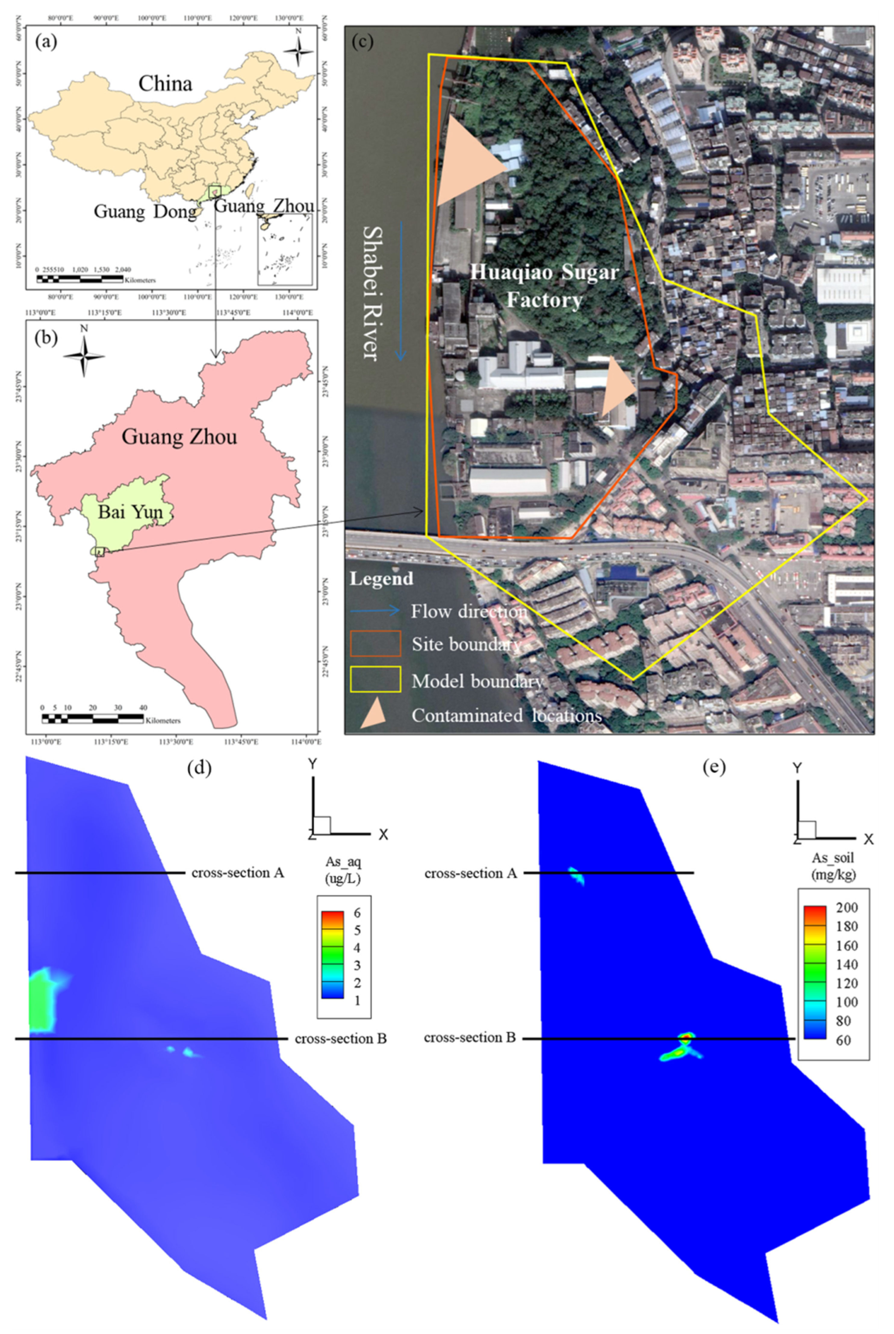
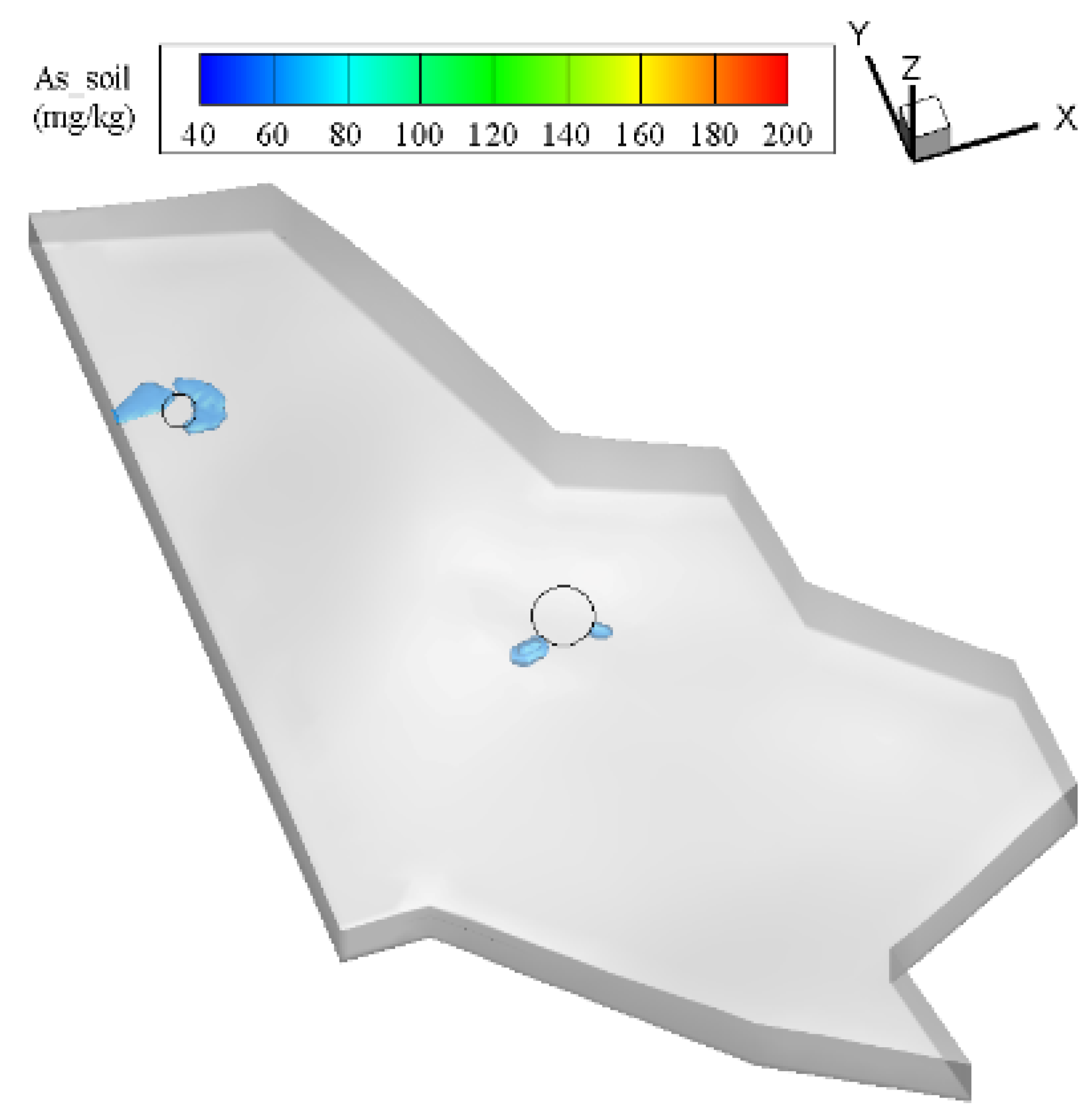
2.2.1. Remediation Site

The remediation site is located in Guangzhou city, Guangdong Province, China, spreading over an area of approximately 124,000 m² (Figure 2). It is in the southern subtropical monsoon climate area, with an average annual temperature of 23 °C, and nearby Shabei River. The average annual precipitation at the site is about 1700 mm, of which 80% occurs in the rainy season from April to September. Shabei River flows at the western boundary of the site, which belongs to the tidal section of the Pearl River Estuary in southern China. The altitude at the site is high in the northeast and low in the southwest. The soil at the site was contaminated with As at several locations (Figure 2), and will be re-developed to establish a research campus after remediation.

2.2.2. Model Domain and Properties

Hydrogeological structure of the model domain for the site was constructed by the high-precision digital elevation model (DEM) from the BIGEMAP software [28] and drilling data from site investigation report, from which the model domain was mesh-discretized. After discretization, the model domain was divided into four layers based on the kriging interpolation using the drilling data and hydrogeological parameters (Table S1). A total number of 69,069 grid cells were discretized with each horizontal grid cell size in the range of 5–30 m. There were 21 vertical layers, divided into two parts. Specifically, the depth of each vertical layer within 8 m underground was 0.5 m, and the depth of remaining vertical layer was 2 m.

In this study, Shabei river was treated as the time-varying specified head boundary at the west side of the model domain. Every four-hour tidal water level taken from National Marine Data and Information Service [29] was used as hydraulic head in the river. The top boundary (ground surface) was specified as the infiltration boundary with the precipitation data taken from literature [30]. No flow boundary was assumed for the bottom of the model domain since the underlying formation is the aquitard. The remaining boundary of the model domain was placed on the watershed divides as the no flux boundary. Since the division of the model domain was based on a watershed approach, the model boundary was larger than site boundary. To determine the initial flow conditions, the model was first burn-in for 20 years to reach a dynamic steady state. Arsenic was the main contaminant in the study site.

The measured aqueous chemical compositions, including As concentrations in Shabei river, were used as the chemical boundary conditions, and the measured aqueous chemical compositions in groundwater were used as initial chemical conditions for the groundwater in the model domain. The distribution of soil As in the study site was obtained from the site investigation report, and spatially interpolated using three-dimensional scatter interpolation software from MATLAB R2019b (Figure 2e). The initial distribution of As concentration in groundwater was assumed to be in equilibrium with solid phase (Figure 2d). The initial distributions of DOC, DO, Fe (II), CO₂, and pH are shown in Figure S1. Various geochemical and biogeochemical reactions that affect As reactive transport were considered in the reactive transport model [31,32]. These reactions are described in supporting information (Text S1). The reaction parameters and boundary conditions as discussed above were summarized in Tables S2 and S3.

Figure 2. The location of the study site including site and modeling boundaries, and contaminated locations (a–c). The initial distributions of arsenic concentrations in groundwater (d) and soil (e). Here, As_aq and As_soil represented groundwater arsenic concentration, soil arsenic concentration, respectively. The cross-sections A and B were the cross-section of the contaminated locations, respectively.

Figure 2. The location of the study site including site and modeling boundaries, and contaminated locations (a–c). The initial distributions of arsenic concentrations in groundwater (d) and soil (e). Here, As_aq and As_soil represented groundwater arsenic concentration, soil arsenic concentration, respectively. The cross-sections A and B were the cross-section of the contaminated locations, respectively.

2.2.3. Implementation of the Model Framework

For the targeted remediation site, numerical simulations under different scenarios of remedial activities found that the partial excavation and replacement of the contaminated soils with clean soils are required to meet the constraint of time for the re-development of the site. However, the amount and locations of the contaminated soils to be excavated can be optimized with the residual contaminated soil left for natural attenuation. At this site, full excavation of the contaminated soil would result in immediate clean-up of the site, but with a significant cost burden. On the other hand, too much contaminated soil left for natural attenuation might result in the long-term risk of groundwater contamination and contaminant discharge to the nearby river beyond the regulatory limits. Therefore, the goal is to find a remediation strategy with a lowest cost that the site can meet regulatory requirements for the re-development of the site. In this study, the amount of the contaminated soil to be excavated was used to calculate the cost for the corresponding remediation strategy. The simulated risk effects of the residual contaminated soils on groundwater quality and contaminant discharge to the nearby river were treated as the remediation outcomes, which were used to establish a relationship between the remediation strategy, outcomes, and cost, which was then used to find an optimal remediation strategy. In this study, the risk standard for As was divided into two levels from the local government (

Table 1. Optimal contaminant limits in this study.

Standard	Contaminant	Unit	Value	Reference
Level I	Arsenic	ug/L	10	[33]
Level II	Arsenic	mg/kg	60	[34]

): level I, the As concentration in groundwater does not exceed 10 ug/L [33]; level II, the As concentration in groundwater is less than 10 ug/L. Meanwhile, the As content in the soil is less than 60 mg/kg [34].

For those complicated cases with multiple contaminants requiring multiple remediation technologies, extensive simulations will be required to find an optimal remediation strategy. To reduce the computational cost, one can select some representative scenarios for simulations, and the results can then be used to train the ML model to establish the relationship of remediation strategy, outcomes, and cost, which can then be used to find an optimal strategy using the global optimization module.

In the ML step, hyperparameters are important metrics whose values are set before starting the learning process. Here, a grid search optimization method is used to adjust the hyperparameters used in RFR to improve the model prediction accuracy [35,36]. In this study, the RFR model under water and soil remediation requirements were created using the Python-based, open-source code Scikit-learn. Table S4 provides the values of the hyperparameter in this study. The parameters used in the optimization step (SCE-UA algorithm) include the number of complexes (P_comp), the maximum number of function evaluations allowed during optimization (n_max), maximum number of evolution loops before convergency (k_stop), and the percentage change allowed in k_stop loops before convergency (P_cento). The specific values of the parameters in the SCE algorithm for this study are provided in Table S5.

3. Results and Discussion

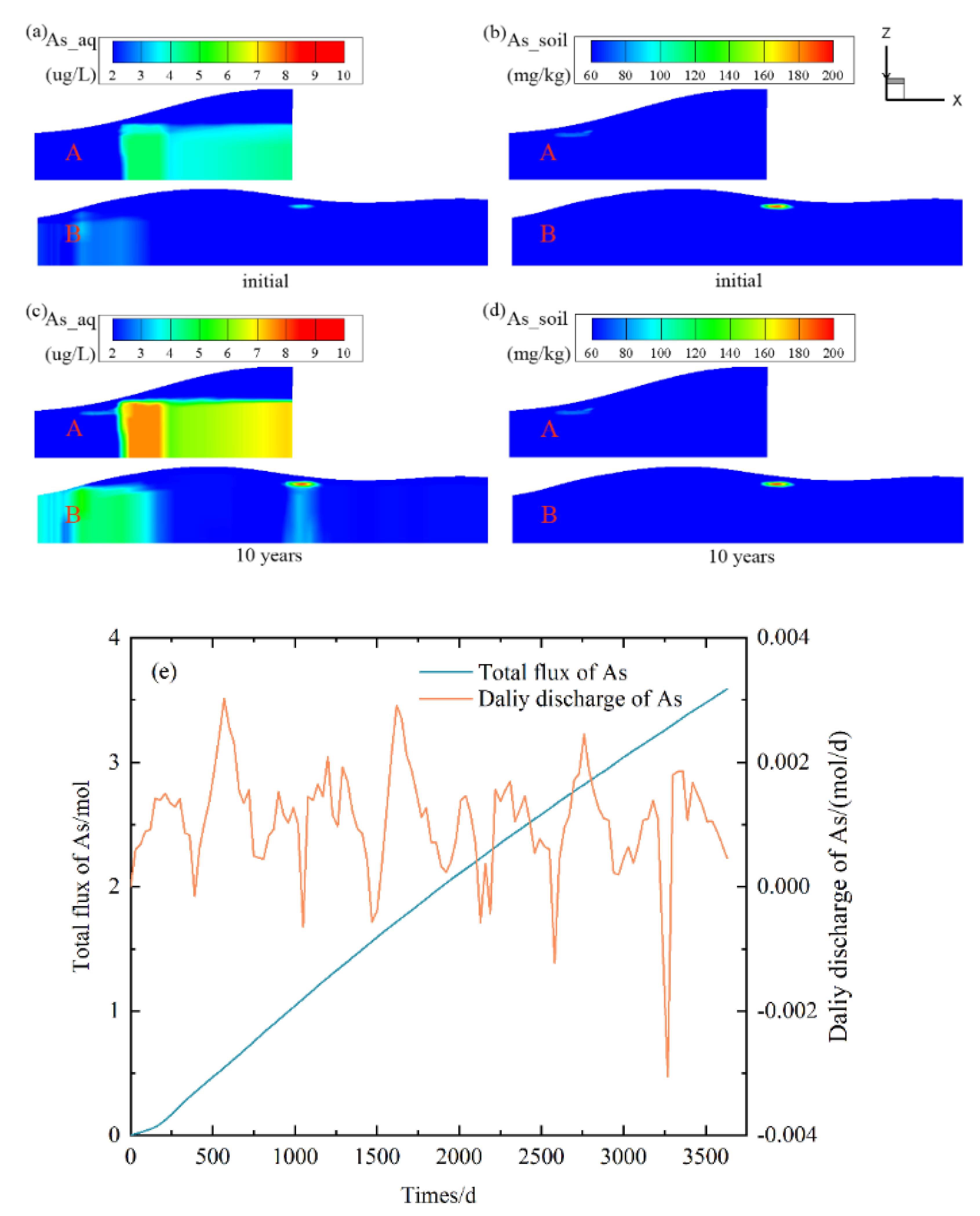
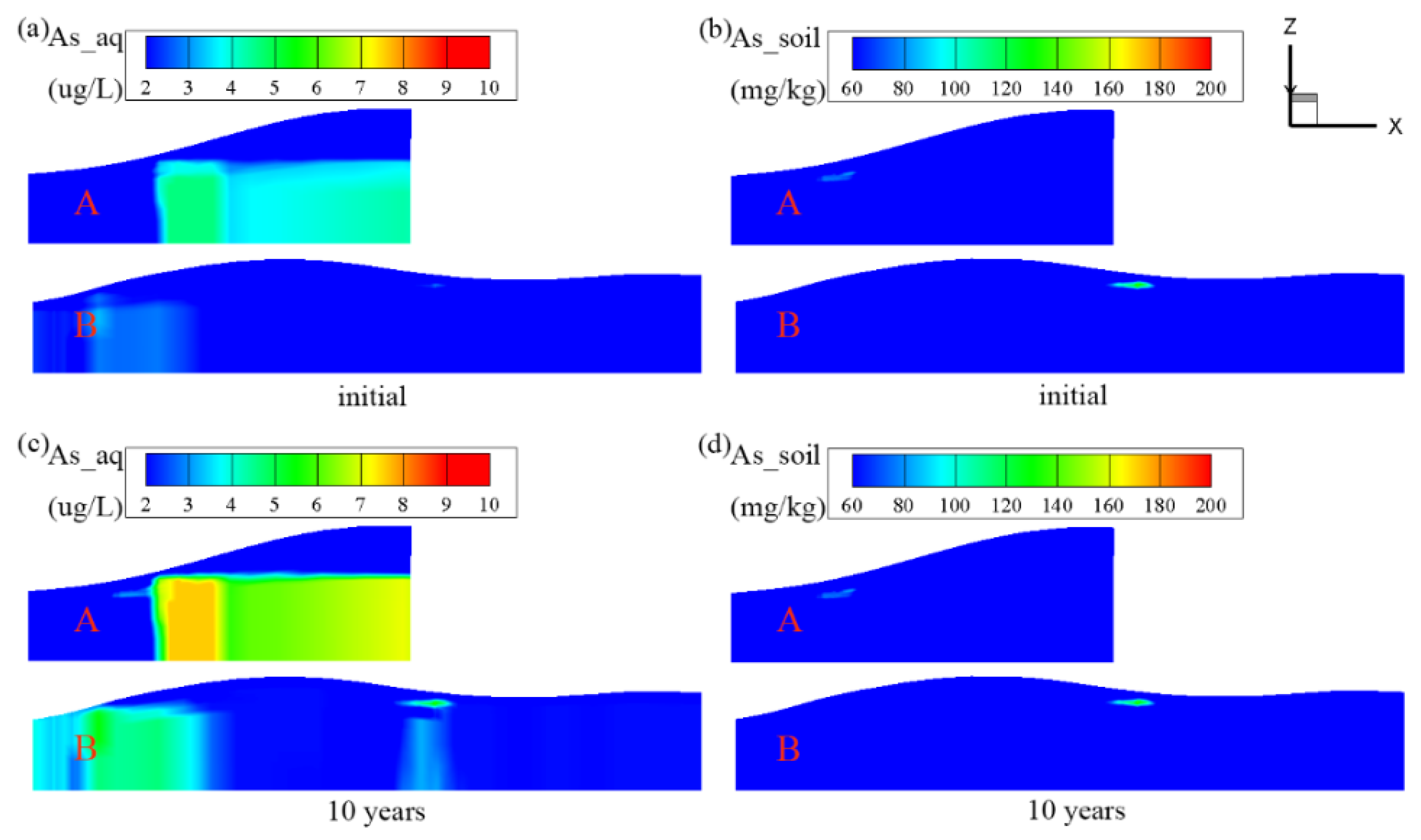
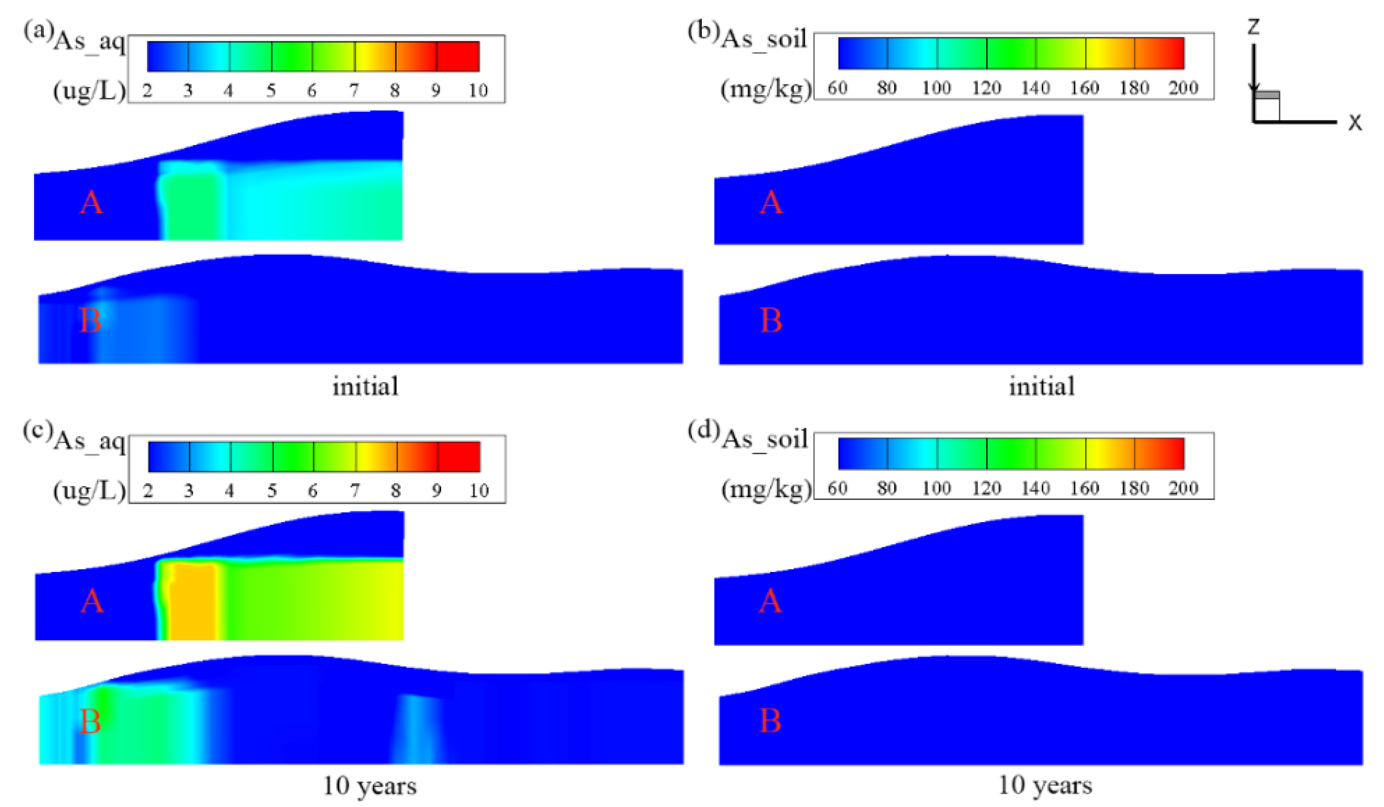
3.1. Results of Natural Attenuation Simulated from the Process-Based Model

The natural attenuation scenario requires the modeling and evaluation of contaminant degradation rates and pathways and the prediction of contaminant concentration at down gradient receptor points, especially when a plume is still expanding/migrating. Figure 3 shows the snapshots of the As concentration distributions, including the contaminated areas, simulated using the process-based model under the natural attenuation condition for the entire site. The initial As concentrations in soil at two locations along cross-sections A and B exceeded the As screening level value (60 mg/kg) in soil with the highest As concentration of 208 mg/kg in cross-section B. All the initial As concentrations in groundwater were below the groundwater standard of 10 ug/L. The result is consistent with the field survey report on the Former Site of Guangzhou Huaqiao Sugar Factory [37]. However, simulation results suggested that the As concentration in groundwater would gradually increase with time as a result of As release from soil when groundwater redox condition changes and the reductive dissolution of As-ferrihydrite in the soil. After 10 years, the highest As concentration in groundwater at cross-section B would exceed 10 ug/L, suggesting that there is a risk of groundwater contamination if the contaminated soil is not treated. On the other hand, the As concentration in the contaminated soil will gradually decrease, but it takes long time to reach below 60 mg/kg. Processes that can affect the natural attenuation of As include adsorption and desorption, as well as site sediment heterogeneity, affecting the flow velocity. The calculated flux of As from the contaminated site to the Shabei river is small and would not increase the As concentration in the river as a result of dilution (Figure 3e). The groundwater mobility in this study site is poor, leading to a very slow migration process of As which takes a long time to achieve the remediation goals. Therefore, the longer attenuation and monitoring time were selected for this specific site. However, this is a site-specific issue, depending on the characteristics of the site and types of contaminants. The primary objective of site modeling is to demonstrate that natural processes of contaminant degradation will reduce contaminant concentrations below regulatory standards or risk-based levels in an appropriate time frame before potential exposure pathways are completed. If the groundwater mobility of the contaminated site is large and the degradation rate of contaminants is fast, such a long simulation time may not be required. In addition, sampling and sample analysis must be conducted during the process to confirm that clean-up is proceeding at rates consistent with cleanup objectives. A long-term monitoring program is underway at the site that will monitor groundwater As concentration. The results can be used to validate approach in future.

These results indicated that active remedial actions, such as the partial excavation and the replacement of the contaminated soil with clean soil, or the establishment of a barrier to isolate the source zone to prevent As dispersion in the soil, are required. The barrier approach would, however, affect groundwater concentration in the isolated area. Therefore, the choice in the source zone is to partially excavate the contaminated soil and that partially left for natural attenuation with the goal to minimize the excavation amount without leading to groundwater contamination.

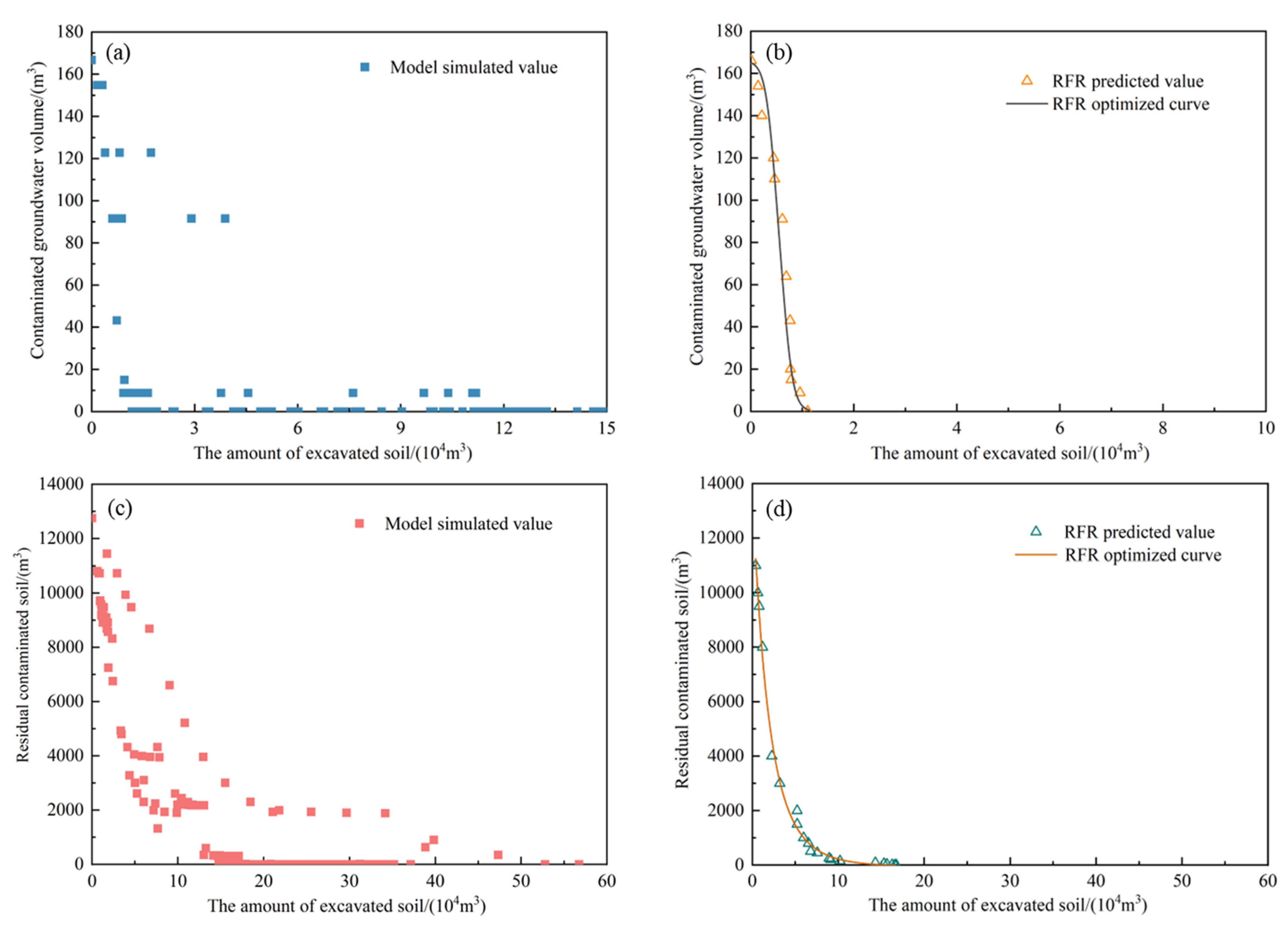
3.2. Results of Excavation Strategies from the Process-Based Model

Figure 4,Figure 5 and Figure 6 show the results of three scenarios with partial excavation of the contaminated soil and partial left for natural attenuation simulated using the process-based model. In scenario 1, 3142 m³ of the highly contaminated soil is removed. The residual contaminated soil still has As concentration as high as 205 mg/kg that can gradually release As to groundwater (Figure 4). After 10 years, the As concentration in groundwater at cross-section B would exceed 10 ug/L, posing a risk to groundwater contamination. When the volume of the excavated soil is increased in scenario 2 to 2.8 times that in scenario 1, the highest As concentration in soils decreases to 135 mg/kg. The residual contaminated soil would still release As to groundwater (Figure 5). However, the As concentration in groundwater is no longer above 10 ug/L. In scenario 3, the contaminated soil is completely excavated (168,077 m³), and both As concentrations in groundwater and soil meet the regulatory requirements after the excavation (Figure 6). Other scenarios with variable volumes of the excavated soil are also simulated (results not shown), generating a set of data linking the remediation cost (volume of excavated soil) and outcomes (aqueous As concentrations, As concentration in residual soil, contaminated volumes of water and soil, and flux discharge to river). These results were used to find an optimal remediation strategy, as described in the next section.

Figure 3. Initial and simulated (after 10 years) distributions of groundwater arsenic concentrations (a,c) and soil arsenic concentrations (b,d) along cross-sections A and B without any soil treatments. Here, As_aq and As_soil represented groundwater arsenic concentration, soil arsenic concentration, respectively. The locations of cross-sections A and B were provided in Figure 2. Plot (e) is the total flux and daily discharge of As from the site to the river.

Figure 3. Initial and simulated (after 10 years) distributions of groundwater arsenic concentrations (a,c) and soil arsenic concentrations (b,d) along cross-sections A and B without any soil treatments. Here, As_aq and As_soil represented groundwater arsenic concentration, soil arsenic concentration, respectively. The locations of cross-sections A and B were provided in Figure 2. Plot (e) is the total flux and daily discharge of As from the site to the river.

Figure 4. Initial distributions of As concentration in groundwater (a) and in soil (b), The simulated distributions of As concentrations in groundwater (c) and in soil (d) after 10 years of the partial excavation of highly contaminated soil (scenario 1). Here, As_aq and As_soil represented groundwater arsenic concentration, soil arsenic concentration, respectively.

Figure 4. Initial distributions of As concentration in groundwater (a) and in soil (b), The simulated distributions of As concentrations in groundwater (c) and in soil (d) after 10 years of the partial excavation of highly contaminated soil (scenario 1). Here, As_aq and As_soil represented groundwater arsenic concentration, soil arsenic concentration, respectively.

Figure 5. Initial distributions of As concentration in groundwater (a) and in soil (b), The simulated distributions of As concentrations in groundwater (c) and in soil (d) after 10 years of the partial excavation of highly contaminated soil (scenario 2). Here, As_aq and As_soil represented groundwater arsenic concentration, soil arsenic concentration, respectively.

Figure 5. Initial distributions of As concentration in groundwater (a) and in soil (b), The simulated distributions of As concentrations in groundwater (c) and in soil (d) after 10 years of the partial excavation of highly contaminated soil (scenario 2). Here, As_aq and As_soil represented groundwater arsenic concentration, soil arsenic concentration, respectively.

Figure 6. Initial distributions of As concentration in groundwater (a) and in soil (b), The simulated distributions of As concentrations in groundwater (c) and in soil (d) after 10 years of the complete excavation of highly contaminated soil (scenario 3). Here, As_aq and As_soil represented groundwater arsenic concentration, soil arsenic concentration, respectively.

Figure 6. Initial distributions of As concentration in groundwater (a) and in soil (b), The simulated distributions of As concentrations in groundwater (c) and in soil (d) after 10 years of the complete excavation of highly contaminated soil (scenario 3). Here, As_aq and As_soil represented groundwater arsenic concentration, soil arsenic concentration, respectively.

3.3. Results of Optimal Remediation Strategy from ML and Optimization Modules

The simulated results from the process-based models (Figure 7a,c) indicated that the volumes of the contaminated groundwater and the residual contaminated soil decrease with the increasing volume of excavated soil. However, for the same volume of the excavated soil, there are multiple of remediation outcomes because there are multiple placement selections for the same volume of the excavated soil at the site. For each specific volume of the excavated soil, there should be one strategy that leads to a minimal volume of contaminated groundwater and residual contaminated soil. For the same volume of the excavated soil, the excavation strategy leading to the mineral volume of contaminated groundwater is not necessarily corresponding to the strategy leading to the minimal volume of the residual contaminated soil. The optimization strategy for this case is then to find the minimal volumes of contaminated groundwater and the residual contaminated soil as a function of the excavated volume of the contaminated soil. Such a function can be obtained from the simulation outcomes using the process-based model and be used by decision makers to select an optimal remediation strategy. However, extensive simulations would be required to generate enough data for each excavated volume of the contaminated soil.

Instead of the extensive simulations using the process-based model, the ML method, RFR, was used in this study to establish the relationship between the excavated volume of the contaminated soil and the minimal volumes of contaminated groundwater and residual contaminated soil. To provide enough data for training the ML model, 341 excavation scenarios were simulated using the process-based model with the data partially shown in (Figure 7a,c). Specifically, the excavation locations, including vertical and horizontal distributions of the excavated soil used in the process-based model as the inputs, the volumes of the contaminated groundwater with As concentration exceeding 10 ug/L, and the volume of the residual contaminated soil with concentration larger than 60 mg/kg were used as the outputs to train the RFR model. The trained model has, respectively, R² and NSE values of 0.9998 and 0.9995 for contaminated groundwater, and 0.9637 and 0.9965 for the residual contaminated soil (Table S6, Figures S2 and S3), indicating the model was well trained.

After training the RFR model, it was then used in the SCE-UA optimization algorithm to find a set of optimal remediation strategies as a function of excavated soil, i.e., minimal volumes of contaminated groundwater and residual contaminated soil as a function of the excavated soil (Figure 7b,d) as well as corresponding horizontal and vertical locations of the excavated soil. Such a function can be used by decision makers to select an optimal remediation strategy based on the cost and remediation requirements. For example, the minimum amount of the contaminated soil that needs to be excavated is 11,068 m³ in order to avoid groundwater contamination with a corresponding excavation location provided in Figure 8. Note that for this relatively simple case, the optimal function can also be obtained from extensive simulations from the process-based model. However, for this case, it took 18 h for each simulation case using the process-based model, while the time cost for a RFR model training and validation was only about 10 s, indicating the magnitude of the reduction of computation burden.

The remediation strategy, as shown in Figure 8, was successfully implemented at the target remediation site. Compared with the complete excavation of the contaminated soils (168,077 m³), the adopted strategy only excavated 6.6% of the total contaminated soil, leading to a significant saving of the remediation cost.

The model framework proposed in this study is also applicable to other heavy metals. In this study, As was the only metallic contaminant in this site while other heavy metal (such as Cd and Hg) were not observed. However, this is a site-specific issue requiring a large amount of site survey data to construct simulation model (e.g., drilling data, contaminant data, tidal water level, DEM, etc.). If Cd and Hg contamination is to be studied, it is necessary to re-locate the contaminated site and collect site survey data to build a new model.

Figure 7. The simulated results of the volume of the contaminated groundwater (a) and the volume of residual contaminated soil (c) as a function of volume the excavated contaminated soil. Symbols are the results from the process-based model. Plot (b) and plot (d) are the optimized profile from the RFR model between the volume of excavated contaminated soil and the minimal volumes of contaminated groundwater (b) and the residual contaminated soil (d).

Figure 7. The simulated results of the volume of the contaminated groundwater (a) and the volume of residual contaminated soil (c) as a function of volume the excavated contaminated soil. Symbols are the results from the process-based model. Plot (b) and plot (d) are the optimized profile from the RFR model between the volume of excavated contaminated soil and the minimal volumes of contaminated groundwater (b) and the residual contaminated soil (d).

Figure 8. The excavation locations corresponding to the minimum amount of the contaminated soil to be excavated to prevent groundwater contamination as described in the text. The As_soil was soil arsenic concentration. The blue blocks are the residual contaminated soil exceeded 60 mg/kg. The black circles are the excavation locations.

Figure 8. The excavation locations corresponding to the minimum amount of the contaminated soil to be excavated to prevent groundwater contamination as described in the text. The As_soil was soil arsenic concentration. The blue blocks are the residual contaminated soil exceeded 60 mg/kg. The black circles are the excavation locations.

4. Conclusions

A computational framework was developed in this study for searching optimal soil and groundwater remediation strategies. The approach relies on the process-based model that can simulate the integrated effects of various remediation approaches on the remediation outcomes. Extensive simulations are, however, required if only the process-based model is used to search for optimal remediation strategies, especially for the sites when multiple remediation technologies are required to restore soil and groundwater systems. The framework uses an ML approach in coupling with an optimization algorithm to expedite the searching process and to reduce the computation cost. The framework is especially useful for searching risk-based remediation approaches that can take the advantage of the natural attenuation potential in soil and groundwater. In such a case, only some of the contaminant sources need to be treated, while others can be left for natural attenuation without generating the risks of groundwater contamination or contaminant discharge to sensitive locations. The framework can provide various alternative remediation strategies for decision makers to select.

The framework was successfully applied at a field site contaminated with As. For this specific site, the framework provided various simulation scenarios of remediation outcomes, from which only the combination of partial excavation of the contaminated soil and partial maintenance for natural attenuation is a viable choice of remediation strategy based on regulatory and site re-development constraints. The optimization problem became to search for excavation volumes and locations that would generate the minimal volume of contaminated groundwater and residual contaminated soil after remediation. Under the constraint that the residual contaminated soil would not cause groundwater contamination and risk to the nearby river, an optimal excavation strategy, including the volume and location, was found. The result was successfully demonstrated at the field site. This site is relatively simple, however, because the field engineering work only involves the excavation of the contaminated soil and replacement with clean soil. The framework can also be applied to other sites with complicated contamination history and multiple contaminants requiring the combination of various active remediation technologies.

References

1. European Environment Agency. Available online: https://www.eea.europa.eu/ (accessed on 1 January 2022).
2. BNS. Bulletin on Natural Survey of Soil Contamination in 2014. 2014. Available online: http://www.gov.cn/xinwen/2014-04/17/content_2661765.htm (accessed on 24 April 2022).
3. Douay, F.; Roussel, H.; Pruvot, C.; Loriette, A.; Fourrier, H. Assessment of a remediation technique using the replacement of contaminated soils in kitchen gardens nearby a former lead smelter in Northern France. Sci. Total Environ. 2008, 401, 29–38. [Google Scholar] [CrossRef] [PubMed]
4. Moon, D.H.; Grubb, D.G.; Reilly, T.L. Stabilization/solidification of selenium-impacted soils using Portland cement and cement kiln dust. J. Hazard. Mater. 2009, 168, 944–951. [Google Scholar] [CrossRef] [PubMed]
5. Hu, W.; Niu, Y.L.; Zhu, H.; Dong, K.; Wang, D.Q.; Liu, F. Remediation of zinc-contaminated soils by using the two-step washing with citric acid and water-soluble chitosan. Chemosphere 2021, 282, 131092. [Google Scholar] [CrossRef] [PubMed]
6. Wei, Y.M.; Wang, F.; Liu, X.; Fu, P.R.; Yao, R.X.; Ren, T.T.; Shi, D.Z.; Li, Y.Y. Thermal remediation of cyanide-contaminated soils: Process optimization and mechanistic study. Chemosphere 2020, 239, 124707. [Google Scholar] [CrossRef]
7. Nejad, Z.D.; Jung, M.C.; Kim, K.H. Remediation of soils contaminated with heavy metals with an emphasis on immobilization technology. Environ. Geochem. Health 2018, 40, 927–953. [Google Scholar] [CrossRef]
8. Gong, Y.Y.; Zhao, D.Y.; Wang, Q.L. An overview of field-scale studies on remediation of soil contaminated with heavy metals and metalloids: Technical progress over the last decade. Water Res. 2018, 147, 440–460. [Google Scholar] [CrossRef]
9. EPA. Use of Monitored Natural Attenuation at Superfund, RCRA Corrective Action, and Underground Storage Tank Sites. OSWER. April 21. OSWER Directive No. 9200.4-17P. 1999. Available online: https://semspub.epa.gov/work/HQ/159152.pdf (accessed on 24 January 2022).
10. Sarkar, D.; Ferguson, M.; Datta, R.; Birnbaum, S. Bioremediation of petroleum hydrocarbons in contaminated soils: Comparison of biosolids addition, carbon supplementation, and monitored natural attenuation. Environ. Pollut. 2005, 136, 187–195. [Google Scholar] [CrossRef]
11. Rugner, H.; Finkel, M.; Kaschl, A.; Bittens, M. Application of monitored natural attenuation in contaminated land management—A review and recommended approach for Europe. Environ. Sci. Policy 2006, 9, 568–576. [Google Scholar] [CrossRef]
12. Khan, F.I.; Husain, T. Risk-based monitored natural attenuation—A case study. J. Hazard. Mater. 2001, 85, 243–272. [Google Scholar] [CrossRef]
13. Mills, R.T.; Lu, C.; Lichtner, P.C.; Hammond, G.E. Simulating subsurface flow and transport on ultrascale computers using PFLOTRAN. J. Phys. Conf. Ser. 2007, 78, 012051. [Google Scholar] [CrossRef]
14. Wu, R.J.; Chen, X.Y.; Hammond, G.; Bisht, G.; Song, X.H.; Huang, M.Y.; Niu, G.Y.; Ferre, T. Coupling surface flow with high-performance subsurface reactive flow and transport code PFLOTRAN. Environ. Modell. Softw. 2021, 137, 104959. [Google Scholar] [CrossRef]
15. Lichtner, P.C.; Hammond, G.E.; Lu, C.; Karra, S.; Bisht, G.; Andre, B.; Mills, R.; Kumar, J. PFLOTRAN User Manual: A Massively Parallel Reactive Flow and Transport Model for Describing Surface and Subsurface Processes. Los Alamos National Laboratory (LANL); U.S. Department of Energy: Washington, DC, USA, 2015. [CrossRef] [Green Version]
16. Breiman, L. Random forests. Mach. Learn. 2001, 45, 5–32. [Google Scholar] [CrossRef] [Green Version]
17. He, S.; Wu, J.H.; Wang, D.; He, X.D. Predictive modeling of groundwater nitrate pollution and evaluating its main impact factors using random forest. Chemosphere 2022, 290, 133388. [Google Scholar] [CrossRef]
18. Dai, L.J.; Ge, J.S.; Wang, L.Q.; Zhang, Q.; Liang, T.; Bolan, N.; Lischeid, G.; Rinklebe, J. Influence of soil properties, topography, and land cover on soil organic carbon and total nitrogen concentration: A case study in Qinghai-Tibet plateau based on random forest regression and structural equation modeling. Sci. Total Environ. 2022, 821, 153440. [Google Scholar] [CrossRef]
19. Harrison, J.W.; Lucius, M.A.; Farrell, J.L.; Eichler, L.W.; Relyea, R.A. Prediction of stream nitrogen and phosphorus concentrations from high-frequency sensors using Random Forests Regression. Sci. Total Environ. 2021, 763, 143005. [Google Scholar] [CrossRef]
20. Li, B.; Yang, G.S.; Wan, R.R.; Hormann, G.; Huang, J.C.; Fohrer, N.; Zhang, L. Combining multivariate statistical techniques and random forests model to assess and diagnose the trophic status of Poyang Lake in China. Ecol. Indic. 2017, 83, 74–83. [Google Scholar] [CrossRef]
21. Guo, B.; Zhang, D.M.; Pei, L.; Su, Y.; Wang, X.X.; Bian, Y.; Zhang, D.H.; Yao, W.Q.; Zhou, Z.X.; Guo, L.Y. Estimating PM2.5 concentrations via random forest method using satellite, auxiliary, and ground-level station dataset at multiple temporal scales across China in 2017. Sci Total Environ 2021, 778, 146288. [Google Scholar] [CrossRef] [PubMed]
22. Breiman, L.; Friedman, J.H.; Olshen, R.A.; Stone, C.J. Classification and Regression Trees, 1st ed.; Routledge: New York, NY, USA, 1984. [Google Scholar] [CrossRef]
23. Rahmati, O.; Choubin, B.; Fathabadi, A.; Coulon, F.; Soltani, E.; Shahabi, H.; Mollaefar, E.; Tiefenbacher, J.; Cipullo, S.; Bin Ahmad, B.; et al. Predicting uncertainty of machine learning models for modelling nitrate pollution of groundwater using quantile regression and UNEEC methods. Sci. Total Environ. 2019, 688, 855–866. [Google Scholar] [CrossRef]
24. Wang, X.; Li, R.; Tian, Y.; Liu, C.X. Watershed-scale water environmental capacity estimation assisted by machine learning. J. Hydrol. 2021, 597, 126310. [Google Scholar] [CrossRef]
25. Duan, Q.Y.; Sorooshian, S.; Gupta, V.K. Optimal Use of the Sce-Ua Global Optimization Method for Calibrating Watershed Models. J. Hydrol. 1994, 158, 265–284. [Google Scholar] [CrossRef]
26. Zhang, Y.Y.; Shao, Q.X. Uncertainty and its propagation estimation for an integrated water system model: An experiment from water quantity to quality simulations. J. Hydrol. 2018, 565, 623–635. [Google Scholar] [CrossRef]
27. Tan, J.W.; Duan, Q.Y.; Gong, W.; Di, Z.H. Differences in parameter estimates derived from various methods for the ORYZA (v3) Model. J. Integr. Agr. 2022, 21, 375–388. [Google Scholar]
28. Chengdu Bigemap Data Processing Ltd. Bigemap. Available online: http://www.bigemap.com/ (accessed on 24 April 2022).
29. China Oceanic Information Network. Available online: http://www.nmdis.org.cn/ (accessed on 1 April 2022).
30. He, J.; Yang, K.; Tang, W.J.; Lu, H.; Qin, J.; Chen, Y.Y.; Li, X. The first high-resolution meteorological forcing dataset for land process studies over China. Sci. Data 2020, 7, 25. [Google Scholar] [CrossRef] [PubMed] [Green Version]
31. Huang, K.; Liu, Y.Y.; Yang, C.; Duan, Y.H.; Yang, X.F.; Liu, C.X. Identification of Hydrobiogeochemical Processes Controlling Seasonal Variations in Arsenic Concentrations Within a Riverbank Aquifer at Jianghan Plain, China. Water Resour. Res. 2018, 54, 4294–4308. [Google Scholar] [CrossRef]
32. Yang, C.; Zhang, Y.K.; Liu, Y.; Yang, X.; Liu, C. Model-Based Analysis of the Effects of Dam-Induced River Water and Groundwater Interactions on Hydro-Biogeochemical Transformation of Redox Sensitive Contaminants in a Hyporheic Zone. Water Resour. Res. 2018, 54, 5973–5985. [Google Scholar] [CrossRef]
33. Environmental Protection Agency, Inorganic Contaminant Accumulation in Potable Water Distribution Systems, Office of Groundwater and Drinking Water, USA. 2006. Available online: https://www.epa.gov/dwreginfo/inorganic-contaminant-accumulation-potable-water-distribution-systems (accessed on 24 April 2022).
34. Ministry of Ecology and Environment of the People’s Republic of China. Soil Environmental Quality-Risk Control Standard for Soil Contamination of Development Land (GB36600-2018); China Environment Publishing Group: Beijing, China, 2018; Volume 6. (In Chinese) [Google Scholar]
35. Huan, J.; Li, H.; Li, M.B.; Chen, B. Prediction of dissolved oxygen in aquaculture based on gradient boosting decision tree and long short-term memory network: A study of Chang Zhou fishery demonstration base, China. Comput. Electron. Agr. 2020, 175, 105530. [Google Scholar] [CrossRef]
36. Pedregosa, F.; Varoquaux, G.; Gramfort, A.; Michel, V.; Thirion, B.; Grisel, O.; Blondel, M.; Prettenhofer, P.; Weiss, R.; Dubourg, V.; et al. Scikit-learn: Machine Learning in Python. J. Mach. Learn. Res. 2011, 12, 2825–2830. [Google Scholar]
37. Guangzhou CAOMUFAN Ecological REsearch Co., Ltd. Caomufan. Available online: https://www.caomufan.com/ (accessed on 1 April 2022).
Figure 1. The framework for designing and optimizing remediation strategies for a contaminated site.
Processes 10 02572 g001