

A Hybrid Fault Diagnosis Approach Using FEM Optimized Sensor Positioning and Machine Learning


Abstract
:1. Introduction
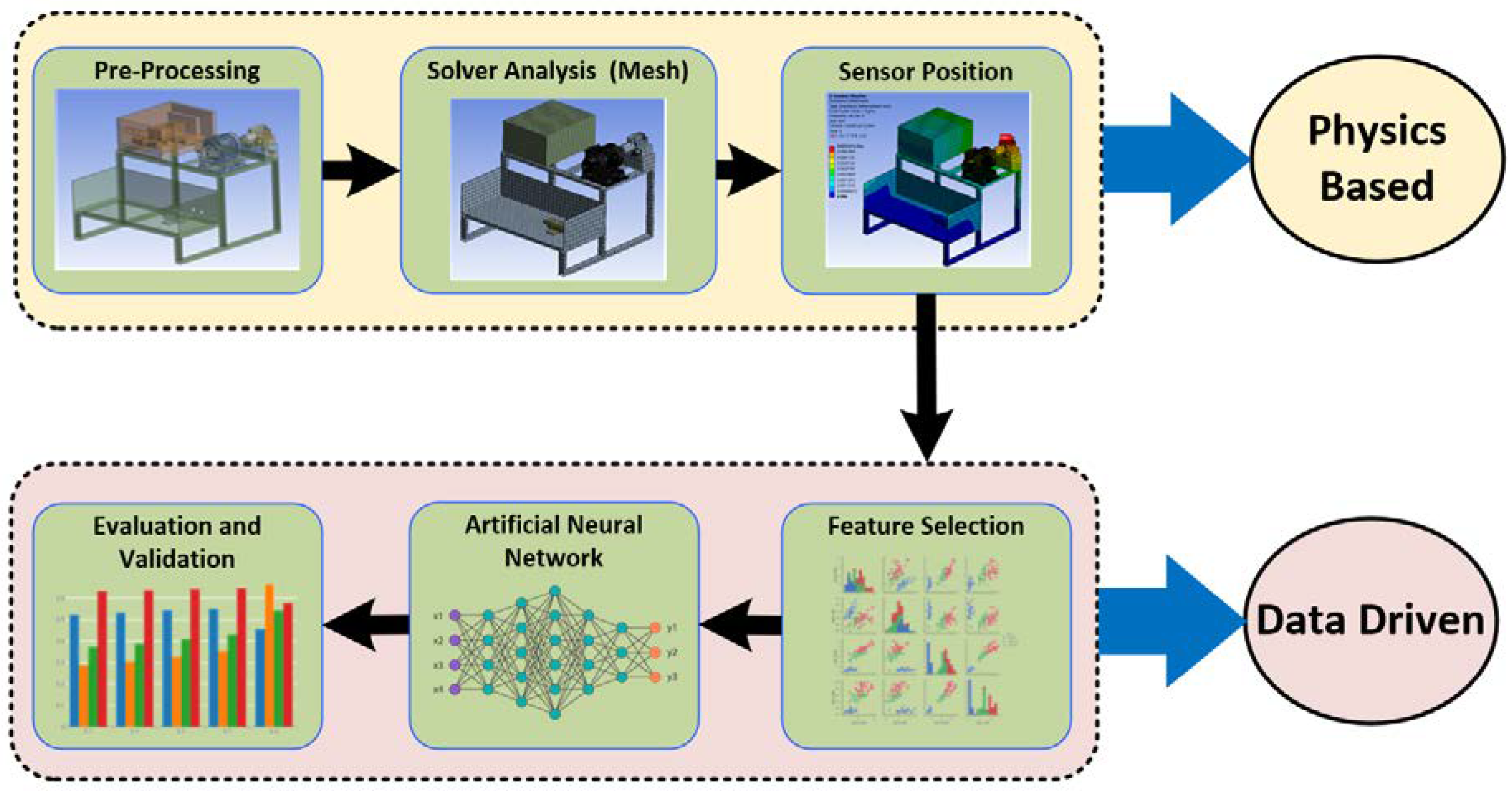
2. Proposed Method
- (1)
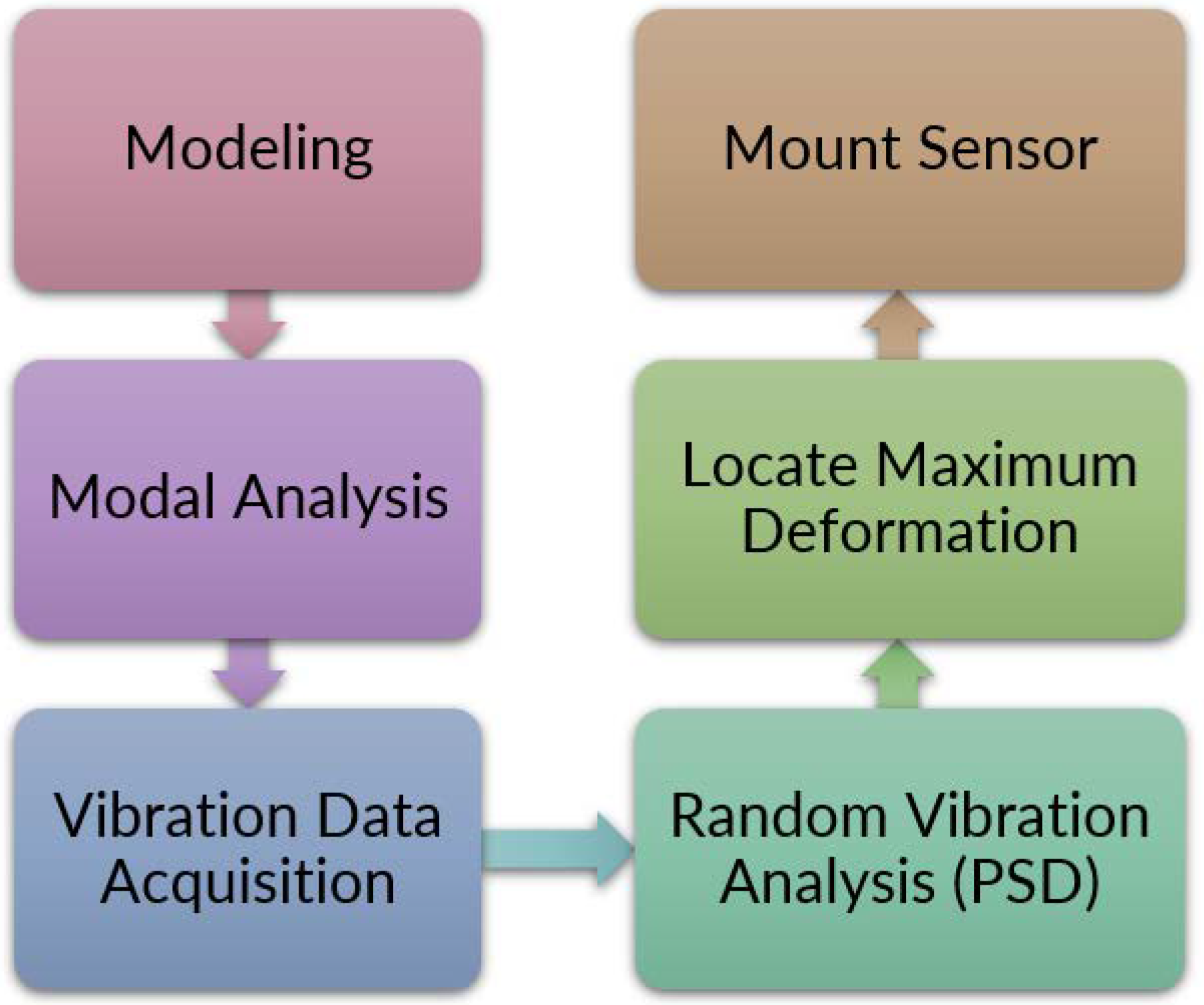
- FEM Analysis for Sensor Positioning
- (2)
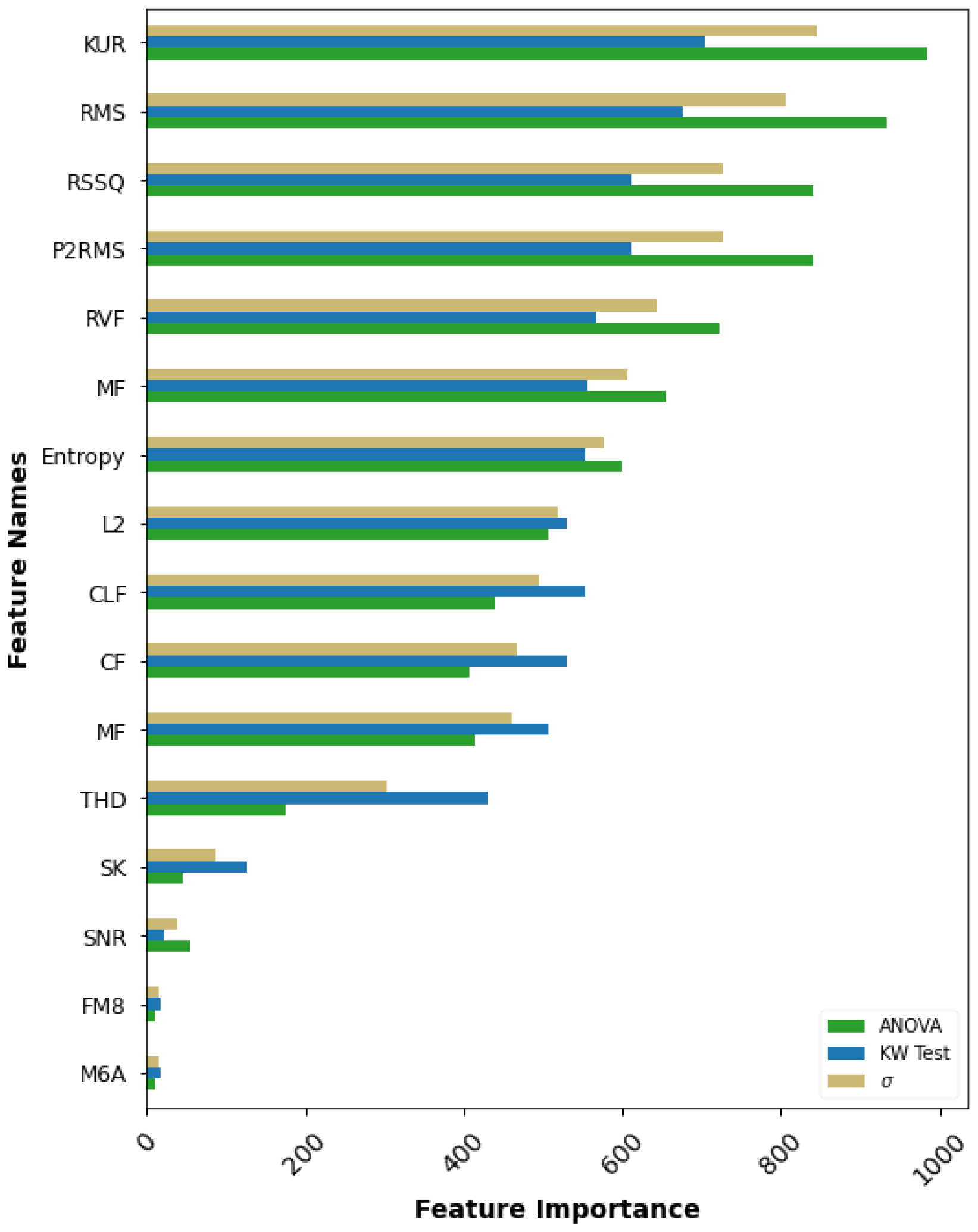
- Selection of Weighty Features
- (3)
- Pattern Recognition and Validation
3. Theoretical Overview
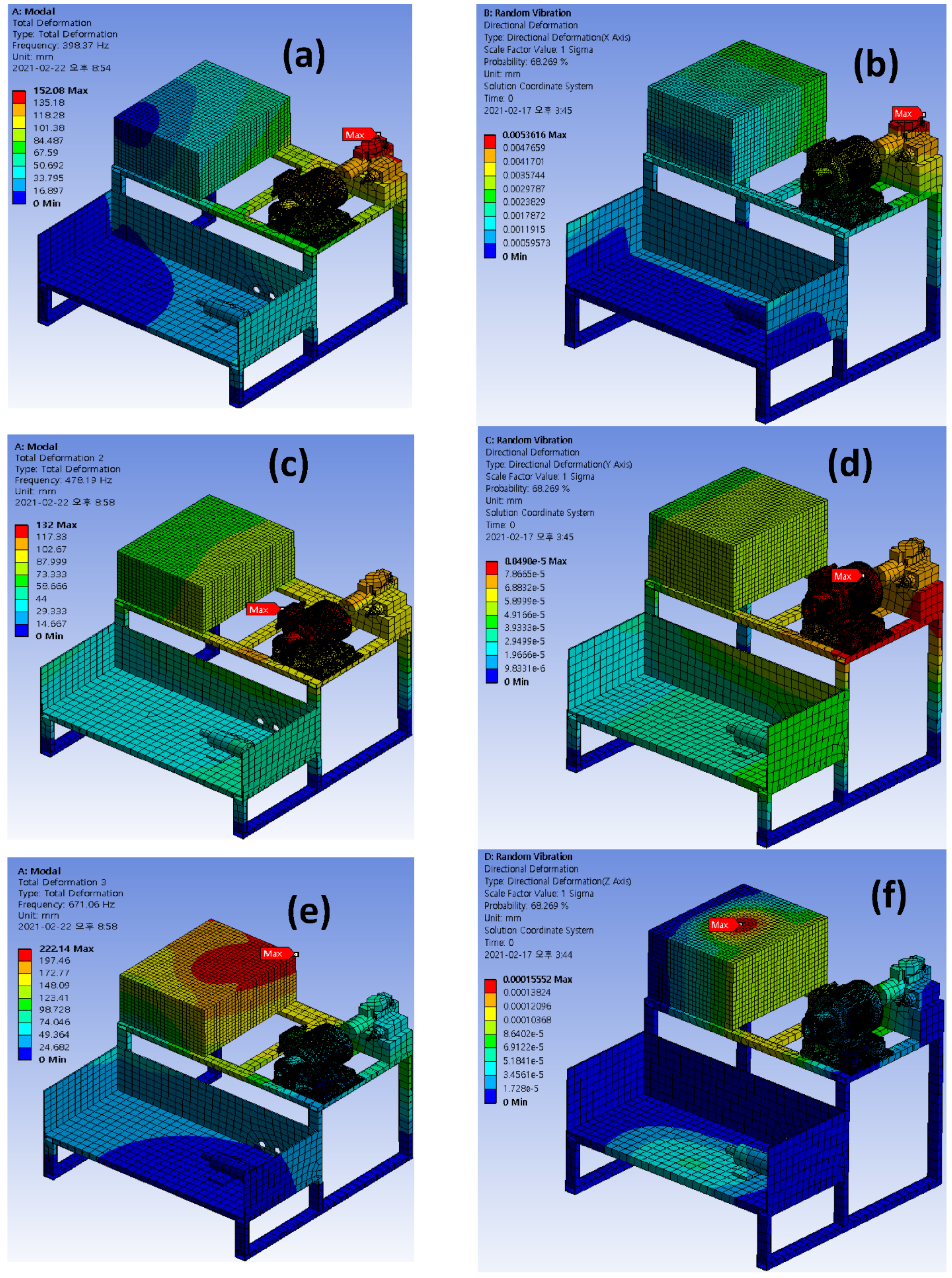
3.1. Finite Element Method (FEM)
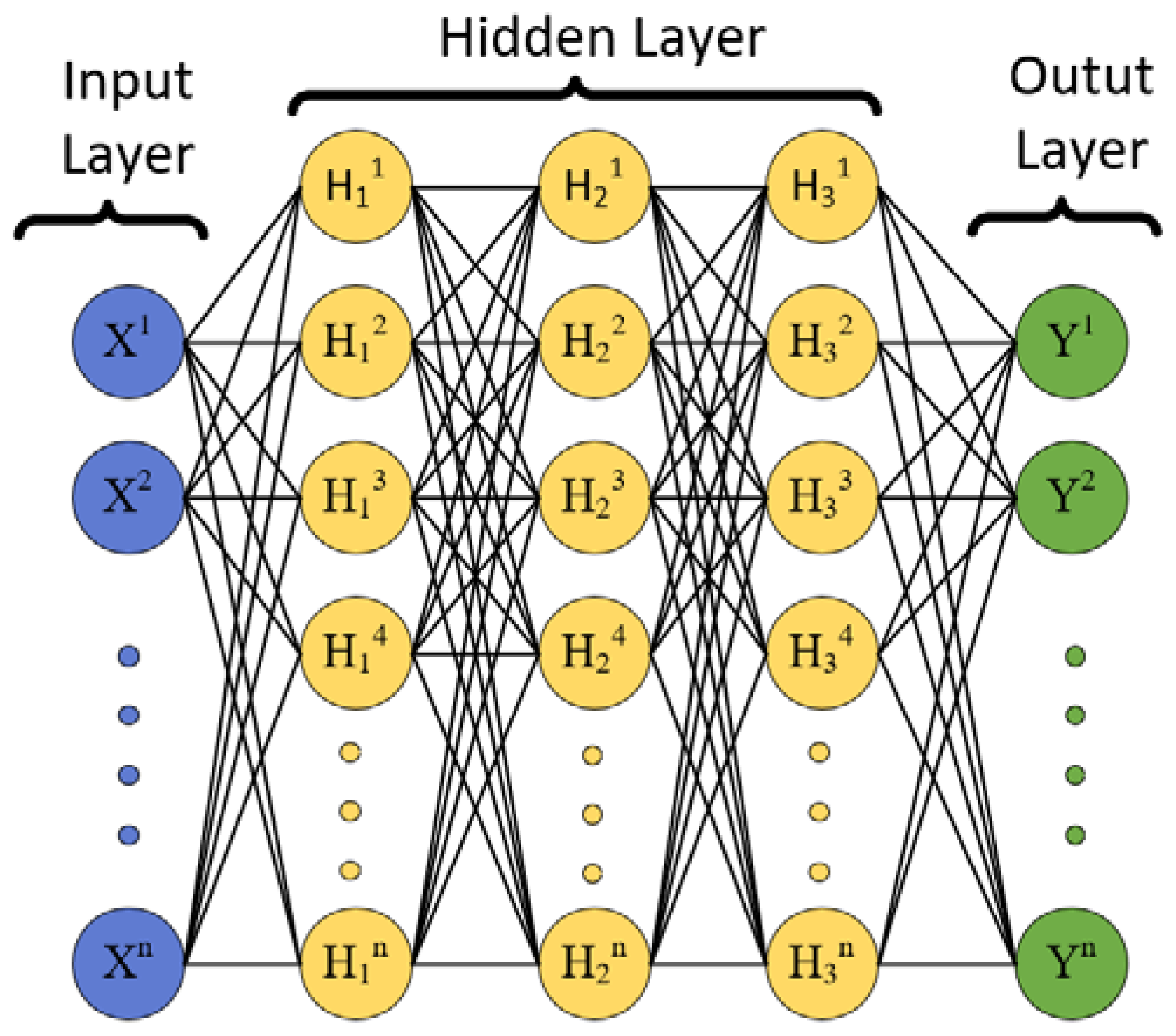
3.2. Pattern Recognition
4. Experiment and Data Description
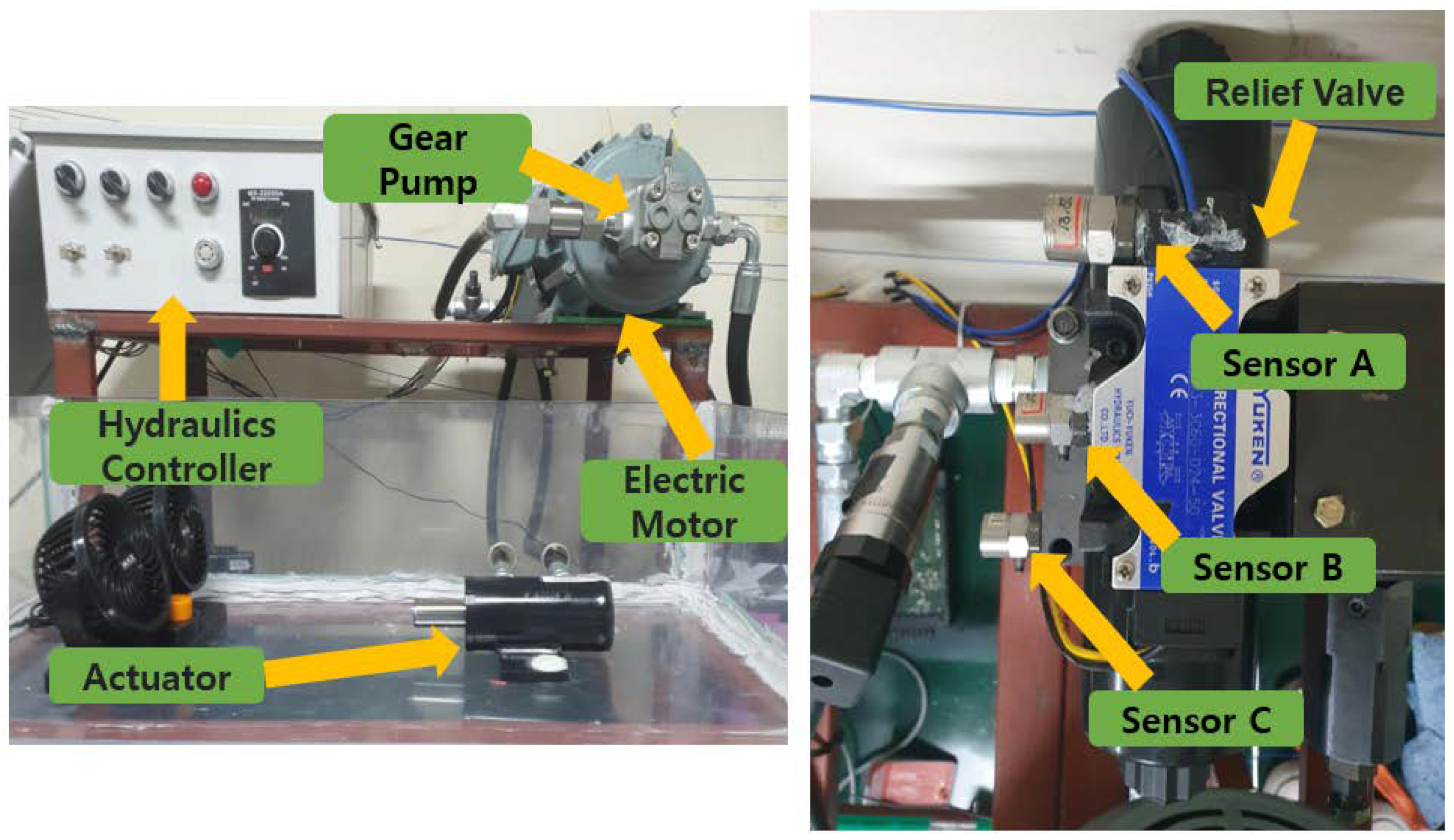
4.1. Test Rig Setup
4.2. Sensor Positioning
5. Result Analysis
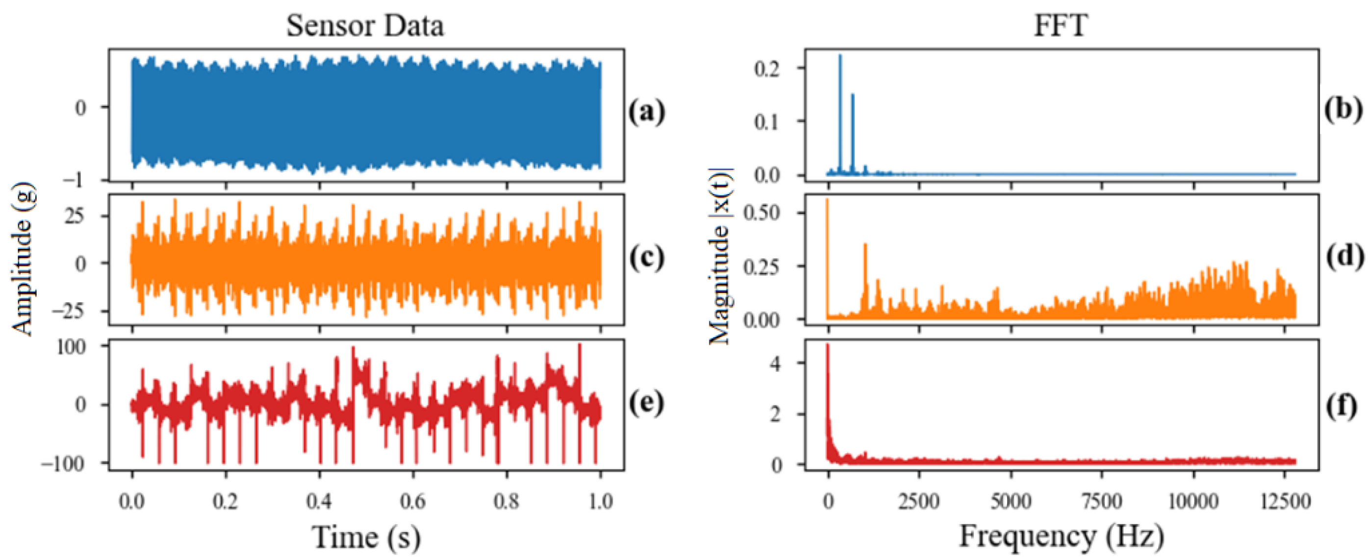
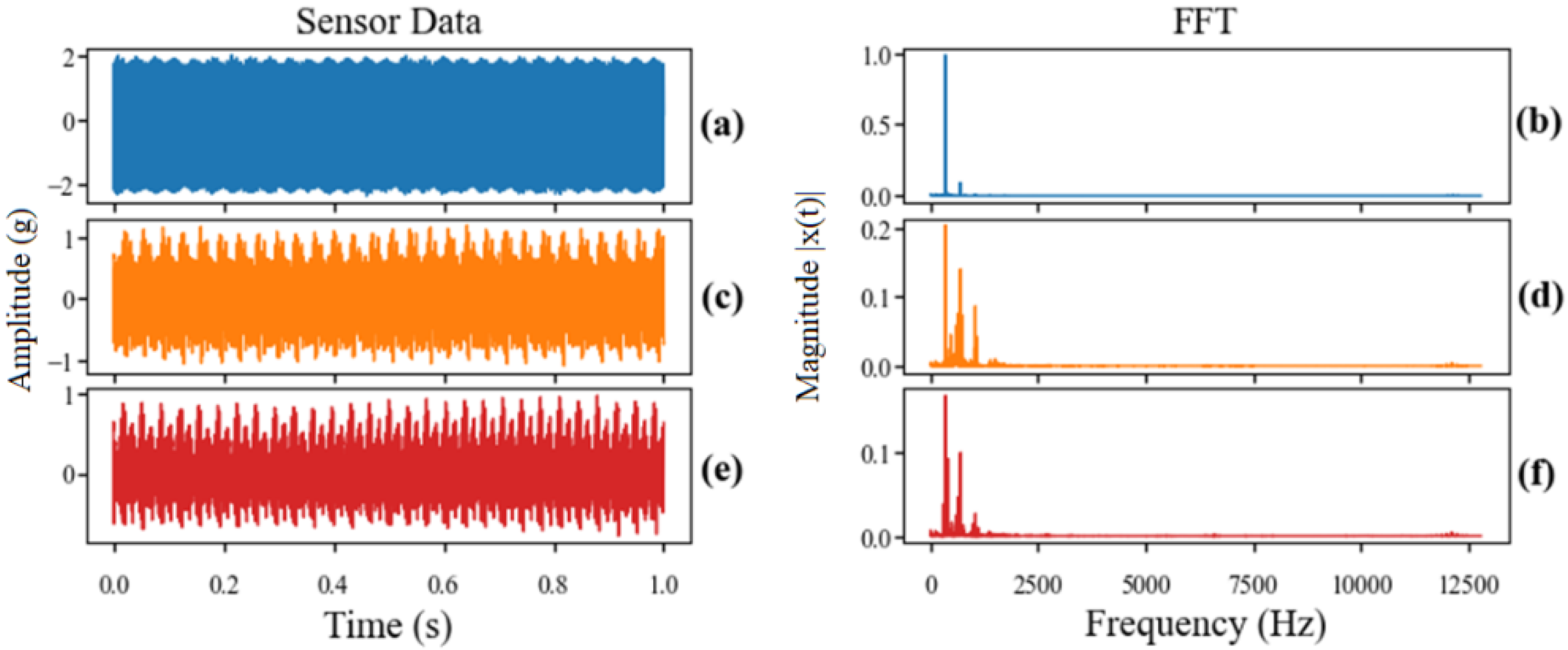
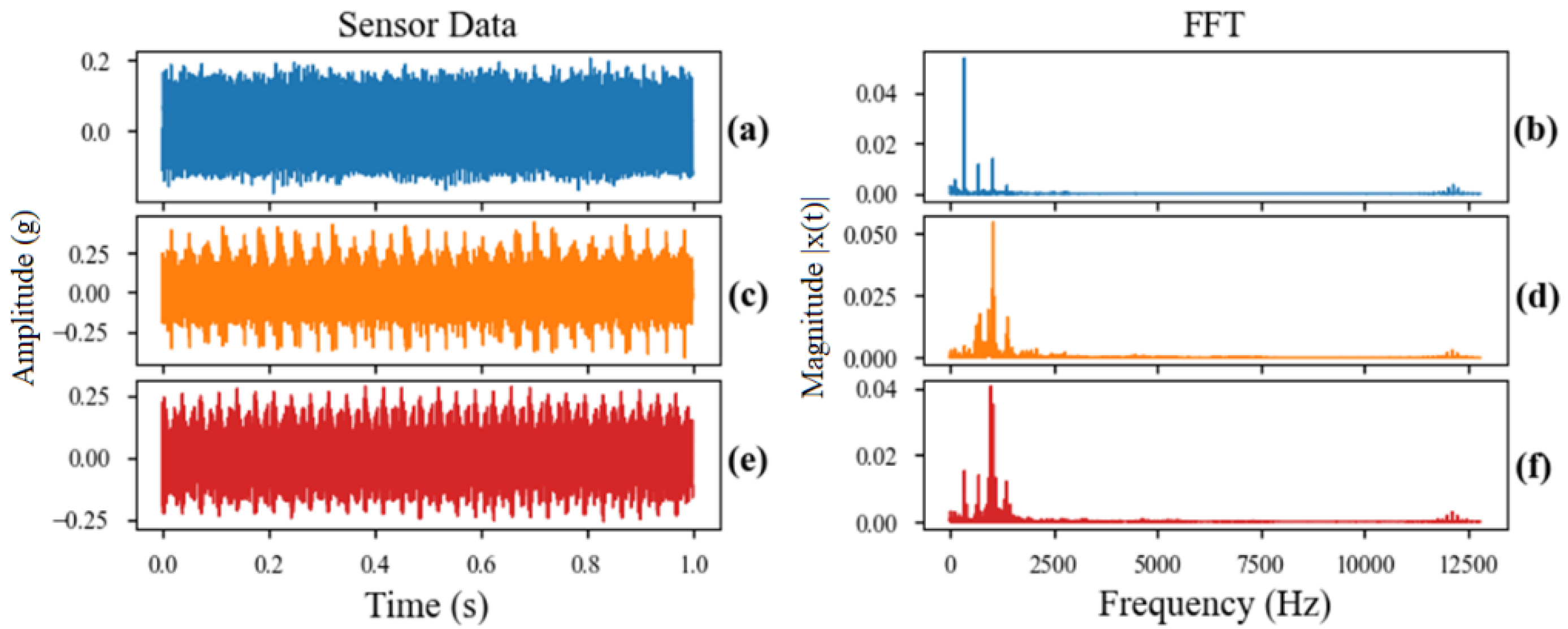
5.1. Data Analysis
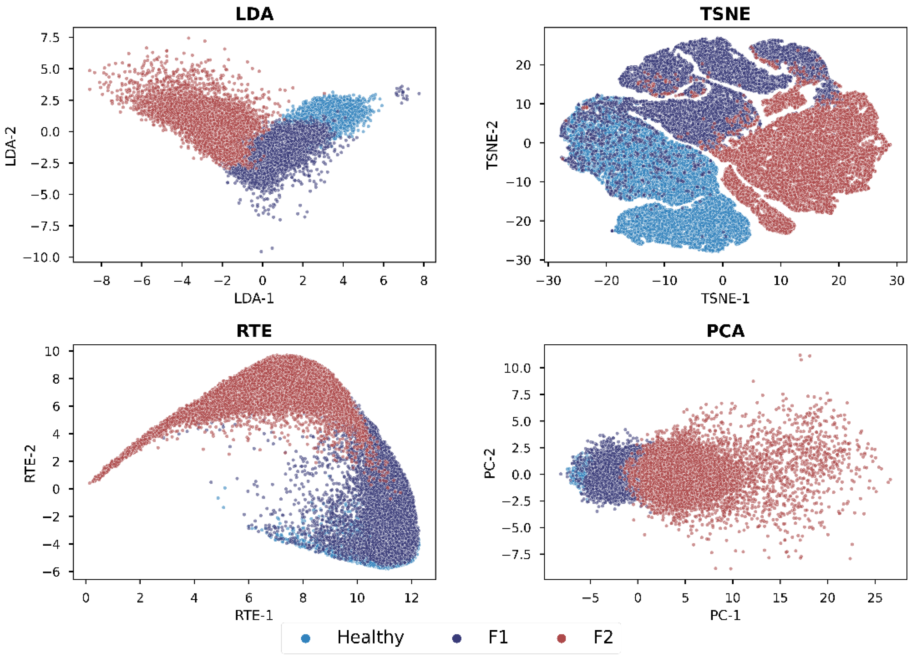
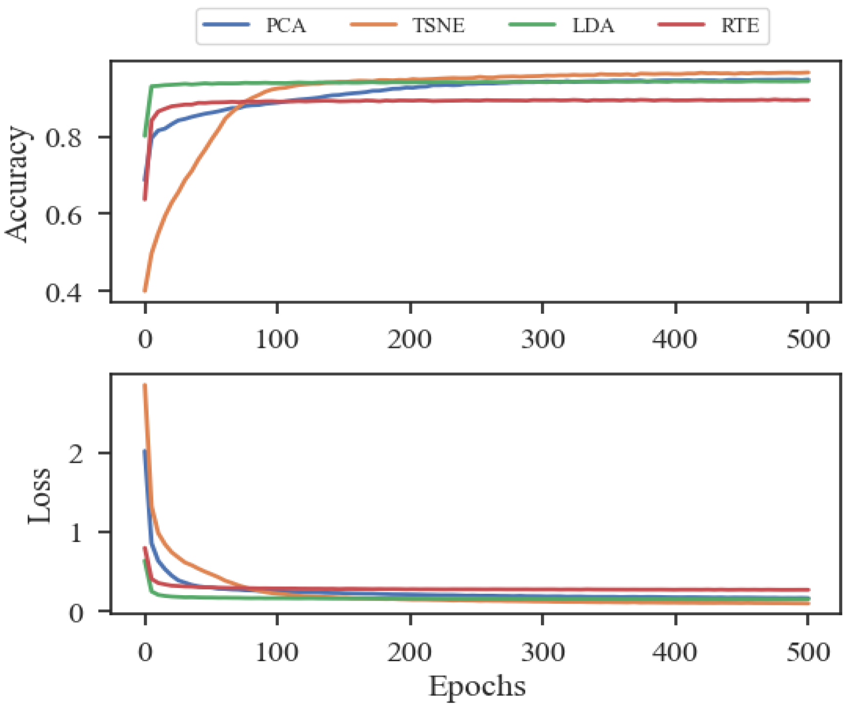
5.2. Failure Pattern Recognition
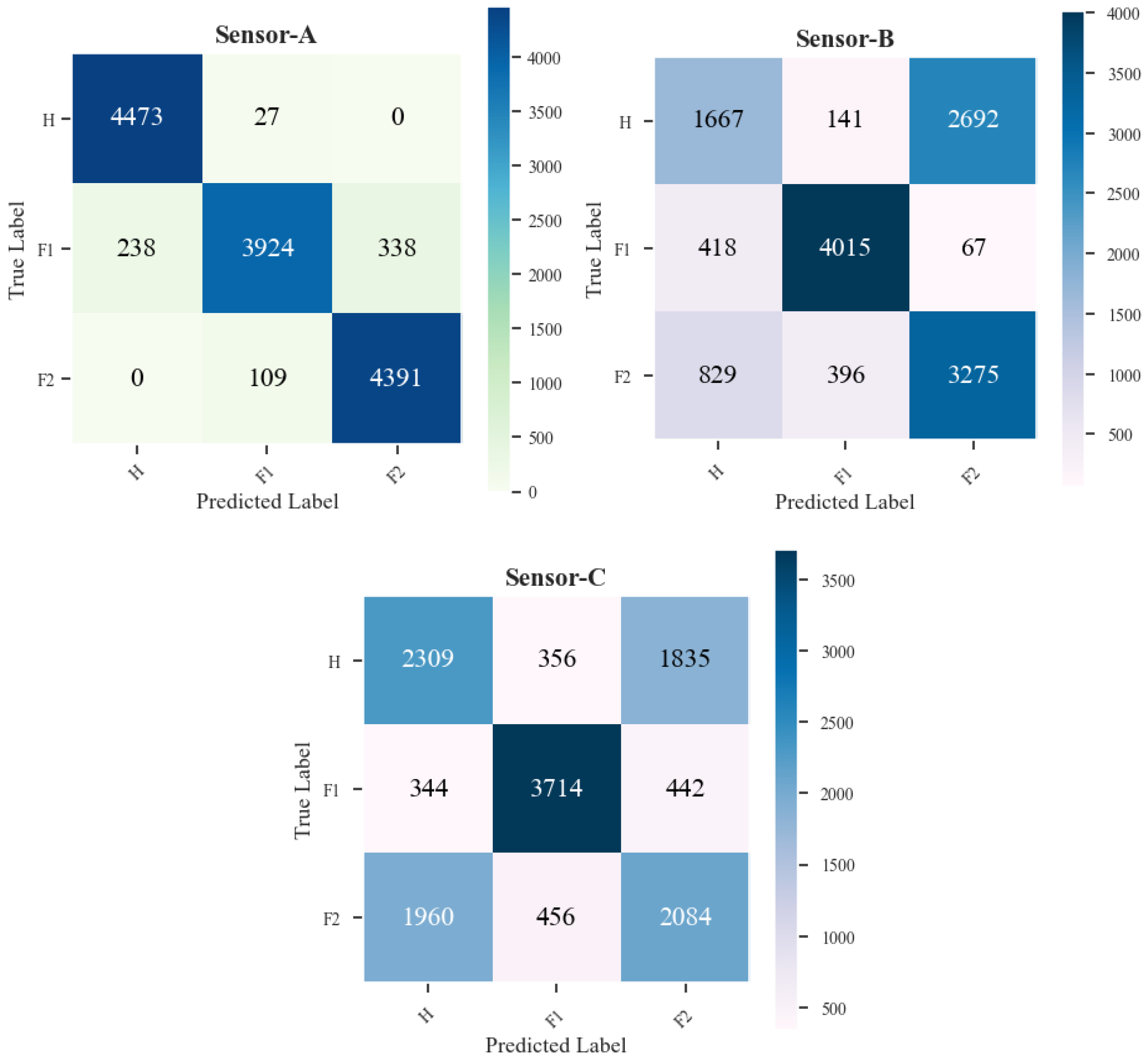
5.3. Validation of the Proposed Method
6. Conclusions
- FEM modeling provides a robust analysis for sensor positioning through a detailed gear-actuator physical model.
- The ANN model is built on two different feature selection approaches ensuring the effectiveness of training data.
Author Contributions
Funding
Institutional Review Board Statement
Informed Consent Statement
Data Availability Statement
Acknowledgments
Conflicts of Interest
References
- Lei, Y.; Yang, B.; Jiang, X.; Jia, F.; Li, N.; Nandi, A.K. Applications of machine learning to machine fault diagnosis: A review and roadmap. Mech. Syst. Signal Process. 2020, 138, 106587. [Google Scholar] [CrossRef]
- Liu, L.; Guo, Q.; Liu, D.; Peng, Y. Data-Driven Remaining Useful Life Prediction Considering Sensor Anomaly Detection and Data Recovery. IEEE Access 2019, 7, 58336–58345. [Google Scholar] [CrossRef]
- Kim, N.-H.; An, D.; Choi, J.-H. Prognostics and Health Management of Engineering Systems; Springer International Publishing: Cham, Switzerland, 2017; pp. 18–138. [Google Scholar]
- Wang, T.; Han, Q.; Chu, F.; Feng, Z. Vibration based condition monitoring and fault diagnosis of wind turbine planetary gearbox: A review. Mech. Syst. Signal Process. 2019, 126, 662–685. [Google Scholar] [CrossRef]
- Krysander, M.; Frisk, E. Sensor placement for fault diagnosis. IEEE Trans. Syst. Man Cybern. Part A Syst. Hum. 2008, 38, 1398–1410. [Google Scholar] [CrossRef]
- Sarrate, R.; Nejjari, F.; Rosich, A. Sensor placement for fault diagnosis performance maximization in Distribution Networks. In Proceedings of the 2012 20th Mediterranean Conference on Control & Automation (MED), Barcelona, Spain, 3–6 July 2012; pp. 110–115. [Google Scholar] [CrossRef]
- Sztyber, A. Sensor Placement for Fault Diagnosis Using Graph of a Process. J. Phys. Conf. Ser. 2017, 783, 012007. [Google Scholar] [CrossRef]
- Wu, J.; Yang, Y.; Wang, P.; Wang, J.; Cheng, J. A novel method for gear crack fault diagnosis using improved analytical-FE and strain measurement. Measurement 2020, 163, 107936. [Google Scholar] [CrossRef]
- Sapena-Bano, A.; Chinesta, F.; Pineda-Sanchez, M.; Aguado, J.; Borzacchiello, D.; Puche-Panadero, R. Induction machine model with finite element accuracy for condition monitoring running in real time using hardware in the loop system. Int. J. Electr. Power Energy Syst. 2019, 111, 315–324. [Google Scholar] [CrossRef]
- Ezzat, A.A.; Tang, J.; Ding, Y. A model-based calibration approach for structural fault diagnosis using piezoelectric impedance measurements and a finite element model. Struct. Health Monit. 2020, 19, 1839–1855. [Google Scholar] [CrossRef]
- Weili, L.; Ying, X.; Jiafeng, S.; Yingli, L. Finite-Element Analysis of Field Distribution and Characteristic Performance of Squirrel-Cage Induction Motor with Broken Bars. IEEE Trans. Magn. 2007, 43, 1537–1540. [Google Scholar] [CrossRef]
- Vaseghi, B.; Takorabet, N.; Meibody-Tabar, F. Fault analysis and parameter identification of permanent-magnet motors by the finite-element method. IEEE Trans. Magn. 2009, 45, 3290–3295. [Google Scholar] [CrossRef]
- Hoang, D.-T.; Kang, H.-J. A survey on Deep Learning based bearing fault diagnosis. Neurocomputing 2018, 335, 327–335. [Google Scholar] [CrossRef]
- Fink, O.; Wang, Q.; Svensen, M.; Dersin, P.; Lee, W.J.; Ducoffe, M. Potential, challenges and future directions for deep learning in prognostics and health management applications. Eng. Appl. Artif. Intell. 2020, 92, 103678. [Google Scholar] [CrossRef]
- Lee, J.; Wu, F.; Zhao, W.; Ghaffari, M.; Liao, L.; Siegel, D. Prognostics and health management design for rotary machinery systems—Reviews, methodology and applications. Mech. Syst. Signal Process. 2014, 42, 314–334. [Google Scholar] [CrossRef]
- Alam Shifat, T.; Jang-Wook, H. Remaining Useful Life Estimation of BLDC Motor Considering Voltage Degradation and Attention-Based Neural Network. IEEE Access 2020, 8, 168414–168428. [Google Scholar] [CrossRef]
- Alam Shifat, T.; Hur, J.-W. ANN Assisted Multi Sensor Information Fusion for BLDC Motor Fault Diagnosis. IEEE Access 2021, 9, 9429–9441. [Google Scholar] [CrossRef]
- He, M.; He, D. Deep Learning Based Approach for Bearing Fault Diagnosis. IEEE Trans. Ind. Appl. 2017, 53, 3057–3065. [Google Scholar] [CrossRef]
- Jing, L.; Zhao, M.; Li, P.; Xu, X. A convolutional neural network based feature learning and fault diagnosis method for the condition monitoring of gearbox. Measurement 2017, 111, 1–10. [Google Scholar] [CrossRef]
- Liang, P.; Deng, C.; Wu, J.; Yang, Z. Intelligent fault diagnosis of rotating machinery via wavelet transform, generative adversarial nets and convolutional neural network. Measurement 2020, 159, 107768. [Google Scholar] [CrossRef]
- Yan, X.; Liu, Y.; Jia, M.; Zhu, Y. A multi-stage hybrid fault diagnosis approach for rolling element bearing under various working conditions. IEEE Access 2019, 7, 138426–138441. [Google Scholar] [CrossRef]
- Alam Shifat, T.; Hur, J.-W. EEMD assisted supervised learning for the fault diagnosis of BLDC motor using vibration signal. J. Mech. Sci. Technol. 2020, 34, 3981–3990. [Google Scholar] [CrossRef]
- Judd, C.M.; McClelland, G.H.; Ryan, C.S. Data Analysis: A Model Comparison Approach to Regression, ANOVA, and Beyond; Routledge: London, UK, 2017. [Google Scholar]
- Rao, S.S.; Atluri, S.N. The Finite Element Method in Engineering. J. Appl. Mech. 1983, 50, 914. [Google Scholar] [CrossRef]
- Meyers, V.J.; Smith, I.M.; Griffiths, D.V. Programming the Finite Element Method. Math. Comput. 1989, 53, 763. [Google Scholar] [CrossRef]
- Reddy, J.N. Introduction to the Finite Element Method; McGraw-Hill Education: New York, NY, USA, 2019. [Google Scholar]
- Saravanan, N.; Ramachandran, K.I. Incipient gear box fault diagnosis using discrete wavelet transform (DWT) for feature extraction and classification using artificial neural network (ANN). Expert Syst. Appl. 2010, 37, 4168–4181. [Google Scholar] [CrossRef]
- Samanta, B.; Al-Balushi, K.R. Artificial Neural Network Based Fault Diagnostics of Rolling Element Bearings Using Time-Domain Features. Mech. Syst. Signal Process. 2003, 17, 317–328. [Google Scholar] [CrossRef]
- Reddy, G.T.; Reddy, M.P.K.; Lakshmanna, K.; Kaluri, R.; Rajput, D.S.; Srivastava, G.; Baker, T. Analysis of Dimensionality Reduction Techniques on Big Data. IEEE Access 2020, 8, 54776–54788. [Google Scholar] [CrossRef]
- Kalsoom, A.; Maqsood, M.; Ghazanfar, M.A.; Aadil, F.; Rho, S. A dimensionality reduction-based efficient software fault prediction using Fisher linear discriminant analysis (FLDA). J. Supercomput. 2018, 74, 4568–4602. [Google Scholar] [CrossRef]
- Ng, A. Machine Learning Yearning. 2018. Available online: http://www.mlyearning.org/ (accessed on 12 September 2021).
- Bengio, Y.; Goodfellow, I.; Courville, A. Deep Learning; MIT Press: Cambridge, MA, USA, 2017; Volume 1. [Google Scholar]
- Alam Shifat, T.; Hur, J. An Improved Stator Winding Short-circuit Fault Diagnosis using AdaBoost Algorithm. In Proceedings of the 2020 International Conference on Artificial Intelligence in Information and Communication (ICAIIC), Fukuoka, Japan, 19–21 February 2020; pp. 382–387. [Google Scholar] [CrossRef]
- Yan, X.; Liu, Y.; Jia, M. A Feature Selection Framework-Based Multiscale Morphological Analysis Algorithm for Fault Diagnosis of Rolling Element Bearing. IEEE Access 2019, 7, 123436–123452. [Google Scholar] [CrossRef]


| Type | Plate | Bracket |
|---|---|---|
| Density | 2700 kg/m3 | 2830 kg/m3 |
| Young’s Modulus | 68.9 GPa | 71.7 GPa |
| Poisson’s Ratio | 0.33 | 0.33 |
| Shear Modulus | 25.9 GPa | 27.0 GPa |
| Yield Strength | 275 MPa | 490 MPa |
| Mode (X) | Frequency (Hz) | Modal Mass (%) | Mode (Y) | Frequency (Hz) | Modal Mass (%) | Mode (Z) | Frequency (Hz) | Modal Mass (%) |
|---|---|---|---|---|---|---|---|---|
| 1 | 578.829 | 45.78 | 1 | 578.829 | 9.32 | 1 | 578.829 | 11.43 |
| 2 | 732.294 | 2.09 | 2 | 732.294 | 68.40 | 2 | 732.294 | 4.37 |
| 3 | 761.892 | 30.06 | 3 | 761.892 | 8.01 | 3 | 761.892 | 21.48 |
| 4 | 1156.5 | 4.32 | 4 | 1156.5 | 7.69 | 4 | 1156.5 | 2.72 |
| 5 | 1338.29 | 8.06 | 5 | 1338.29 | 0.37 | 5 | 1338.29 | 0.11 |
| 6 | 2064.31 | 1.60 | 6 | 2064.31 | 0.15 | 6 | 2064.31 | 8.83 |
| 7 | 2133.15 | 1.88 | 7 | 2133.15 | 0.01 | 7 | 2133.15 | 1.42 |
| 8 | 2584.81 | 1.10 | 8 | 2584.81 | 0.00 * | 8 | 2584.81 | 0.42 |
| 9 | 2646.56 | 0.07 | 9 | 2646.56 | 0.10 | 9 | 2646.56 | 0.14 |
| 10 | 2942.73 | 0.00 * | 10 | 2942.73 | 2.05 | 10 | 2942.73 | 1.05 |
| 11 | 3134.17 | 0.02 | 11 | 3134.17 | 0.03 | 11 | 3134.17 | 3.38 |
| 12 | 3295.8 | 0.01 | 12 | 3295.8 | 1.01 | 12 | 3295.8 | 0.12 |
| 13 | 3597.87 | 0.12 | 13 | 3597.87 | 0.16 | 13 | 3597.87 | 6.96 |
| 14 | 3843.53 | 0.42 | 14 | 3843.53 | 0.17 | 14 | 3843.53 | 18.63 |
| 15 | 4053.49 | 0.88 | 15 | 4053.49 | 0.00 * | 15 | 4053.49 | 5.73 |
| 16 | 4379.57 | 0.24 | 16 | 4379.57 | 0.01 | 16 | 4379.57 | 0.60 |
| 17 | 4638.19 | 0.13 | 17 | 4638.19 | 0.03 | 17 | 4638.19 | 1.92 |
| 18 | 4861.53 | 0.26 | 18 | 4861.53 | 0.01 | 18 | 4861.53 | 0.48 |
| 19 | 4975.44 | 0.17 | 19 | 4975.44 | 0.05 | 19 | 4975.44 | 1.29 |
| 20 | 5746.16 | 0.10 | 20 | 5746.16 | 0.00 * | 20 | 5746.16 | 0.88 |
| Domains | Feature Names |
|---|---|
| Time Domain | Mean, Peak-to-Peak (P2P), Root Mean Square (RMS), Root Sum of Squares (RSSQ), Standard Deviation (STD), Kurtosis (KUR), Skewness (SKEW), L1 Norm (L1), L2 Norm (L2), Peak to RMS (P2RMS), Crest Factor (CF), Shape Factor (SF), Margin Factor (MF), Clearance Factor (CLF), FM4, FM8, M6A. |
| Frequency Domain | Peak Frequency (PF), Total Harmonic Distortion (THD), Spectral Skewness (SS), Spectral Kurtosis (SK), Entropy, Root Variance Frequency (RVF), SNR. |
| Label | Feature Name | Mathematical Expression | Label | Feature Name | Mathematical Expression |
|---|---|---|---|---|---|
| F1 | Kurtosis | F5 | L2-Norm | ||
| F2 | RMS | F6 | Root Variance Frequency | ||
| F3 | Root Sum of Squares | F7 | Entropy | ||
| F4 | Peak-to-RMS | F8 | Mean Frequency |
| Sensor Position | Metrics | H | F1 | F2 |
|---|---|---|---|---|
| Sensor A | Precision | 0.95 | 0.97 | 0.93 |
| Recall | 0.99 | 0.87 | 0.98 | |
| F1-Score | 0.97 | 0.92 | 0.95 | |
| Accuracy | 0.95 | |||
| Sensor B | Precision | 0.57 | 0.88 | 0.54 |
| Recall | 0.37 | 0.89 | 0.73 | |
| F1-Score | 0.45 | 0.89 | 0.62 | |
| Accuracy | 0.66 | |||
| Sensor C | Precision | 0.50 | 0.82 | 0.48 |
| Recall | 0.51 | 0.83 | 0.46 | |
| F1-Score | 0.51 | 0.82 | 0.47 | |
| Accuracy | 0.60 | |||
Publisher’s Note: MDPI stays neutral with regard to jurisdictional claims in published maps and institutional affiliations. |
© 2022 by the authors. Licensee MDPI, Basel, Switzerland. This article is an open access article distributed under the terms and conditions of the Creative Commons Attribution (CC BY) license (https://creativecommons.org/licenses/by/4.0/).
Share and Cite
Jung, S.J.; Shifat, T.A.; Hur, J.-W. A Hybrid Fault Diagnosis Approach Using FEM Optimized Sensor Positioning and Machine Learning. Processes 2022, 10, 1919. https://doi.org/10.3390/pr10101919
Jung SJ, Shifat TA, Hur J-W. A Hybrid Fault Diagnosis Approach Using FEM Optimized Sensor Positioning and Machine Learning. Processes. 2022; 10(10):1919. https://doi.org/10.3390/pr10101919
Chicago/Turabian StyleJung, Sang Jin, Tanvir Alam Shifat, and Jang-Wook Hur. 2022. "A Hybrid Fault Diagnosis Approach Using FEM Optimized Sensor Positioning and Machine Learning" Processes 10, no. 10: 1919. https://doi.org/10.3390/pr10101919