
LARF: Two-Level Attention-Based Random Forests with a Mixture of Contamination Models


Higher School of Artificial Intelligence, Peter the Great St.Petersburg Polytechnic University, Polytechnicheskaya, 29, 195251 St. Petersburg, Russia
*
Author to whom correspondence should be addressed.
†
These authors contributed equally to this work.
Informatics 2023, 10(2), 40; https://doi.org/10.3390/informatics10020040
Submission received: 11 December 2022
/
Revised: 14 April 2023
/
Accepted: 21 April 2023
/
Published: 28 April 2023
(This article belongs to the Section Machine Learning)
Abstract
:This paper provides new models of the attention-based random forests called LARF (leaf attention-based random forest). The first idea behind the models is to introduce a two-level attention, where one of the levels is the “leaf” attention, and the attention mechanism is applied to every leaf of trees. The second level is the tree attention depending on the “leaf” attention. The second idea is to replace the softmax operation in the attention with the weighted sum of the softmax operations with different parameters. It is implemented by applying a mixture of Huber’s contamination models and can be regarded as an analog of the multi-head attention, with “heads” defined by selecting a value of the softmax parameter. Attention parameters are simply trained by solving the quadratic optimization problem. To simplify the tuning process of the models, it is proposed to convert the tuning contamination parameters into trainable parameters and to compute them by solving the quadratic optimization problem. Many numerical experiments with real datasets are performed for studying LARFs. The code of the proposed algorithms is available.
1. Introduction
Several crucial improvements in neural networks have been made in recent years. One of them is the attention mechanism, which has significantly improved classification and regression models in many machine learning areas, including the natural language processing models, computer vision, etc. [1,2,3,4,5]. The idea behind the attention mechanism is to assign weights to features or examples in accordance with their importance and their impact on the model predictions. The attention weights are learned by incorporating an additional feedforward neural network within a neural network architecture. Additionally, the success of the attention models as components of the neural network motivates one to extend this approach to other machine learning models different from neural networks, for example, to random forests (RFs) [6]. Following this idea, a new model called the attention-based random forest (ABRF) has been developed [7,8]. This model incorporates the attention mechanism into ensemble-based models such as RFs and the gradient boosting machine [9,10]. The ABRF models stem from the interesting interpretation [1,11] of the attention mechanism through the Nadaraya–Watson kernel regression model [12,13]. The Nadaraya–Watson regression model learns a non-linear function by using a weighted average of data using a specific normalized kernel as a weighting function. A detailed description of the model can be found in Section 3. According to [7,8], attention weights in the Nadaraya–Watson regression are assigned to decision trees in an RF depending on examples which fall into leaves of trees. Weights in ABRF have trainable parameters and use Huber’s -contamination model [14] for defining the attention weights. Huber’s -contamination model can be regarded as a set of convex combinations of probability distributions, where one of the distributions is considered as a set of trainable attention parameters. A detailed description of the model is provided in Section 5.1. In accordance with the -contamination model, each attention weight consists of two parts: the softmax operation with the tuning coefficient and the trainable bias of the softmax weight with coefficient . One of the improvements of ABRF, which has been proposed in [15], is based on joint incorporating self-attention and attention mechanisms into the RF. The proposed models outperform ABRF, but this outperformance is not sufficient, because this model provided inferior results for several datasets. Therefore, we propose a set of models which can be regarded as extensions of ABRF and which are based on two main ideas.
The first idea is to introduce a two-level attention, where one of the levels is the “leaf” attention, i.e., the attention mechanism is applied to every leaf of a tree. As a result, we obtain the attention weights assigned to leaves and the attention weights assigned to trees. The attention weights of trees depend on the corresponding weights of leaves which belong to these trees. In other words, the attention at the second level depends on the attention at the first level, i.e., we obtain the attention of the attention. Due to the “leaf” attention, the proposed model will be abbreviated as LARF (leaf attention-based random forest).
One of the peculiarities of LARFs is using a mixture of Huber’s -contamination models instead of the single contamination model, as has been conducted in ABRF. This peculiarity stems from the second idea behind the model, which takes into account the softmax operation with different parameters. In fact, we replace the standard softmax operation by the weighted sum of the softmax operations with different parameters. With this idea, we achieve two goals. First of all, we partially solve the problem of the tuning parameters of the softmax operations which are a part of the attention operations. Each value of the tuning parameter from the predefined set (from the predefined grid) is used in a separate softmax operation. Then, weights of the softmax operations in the sum are trained jointly while training other parameters. This approach can also be interpreted as the linear approximation of the softmax operations with trainable weights and with different values of tuning parameters. However, a more interesting goal is that some analogs of the multi-head attention [16] are implemented by using the mixture of contamination models, where “heads” are defined by selecting a value of the corresponding softmax operation parameter.
Additionally, in contrast to ABRF [8], where the contamination parameter of Huber’s model was a tuning parameter, the LARF model considers this parameter as the training one. This allows us to significantly reduce the model tuning time and avoid the enumeration of the parameter values in accordance with the grid. The same is implemented for the mixture of the Huber’s models.
Different configurations of LARF produce a set of models, which depend on trainable and tuning parameters of the two-level attention and on algorithms for their calculation.
We investigate two types of RFs in the experiments: original RFs and Extremely Randomized Trees (ERT) [17]. According to [17], the ERT algorithm chooses a split point randomly for each feature at each node and then selects the best split among these. In contrast to ERTs, original RFs choose the most optimal (not random) split of a set of features at each node in accordance with a criterion, for example, with the Gini impurity [6].
Our contributions can be summarized as follows:
- We propose new two-level attention-based RF models, where the attention mechanism at the first level is applied to every leaf of trees, the attention at the second level incorporates the “leaf” attention, and it is applied to trees. The training of the two-level attention is reduced to solving the standard quadratic optimization problem.
- A mixture of Huber’s -contamination models is used to implement the attention mechanism at the second level. The mixture allows us to replace a set of tuning attention parameters (the temperature parameters of the softmax operations) with trainable parameters, whose optimal values are computed by solving the quadratic optimization problem. Moreover, this approach can be regarded as an analog of the multi-head attention.
- We propose an approach to convert the tuning contamination parameters ( parameters) in the mixture of the -contamination models into trainable parameters. Their optimal values are also computed by solving the quadratic optimization problem.
Many numerical experiments with real datasets are performed for studying LARFs. They demonstrate outperforming results of some LARF modifications. The code of the proposed algorithms can be found at https://github.com/andruekonst/leaf-attention-forest (accessed on 20 April 2023).
This paper is organized as follows. The related work can be found in Section 2. A brief introduction to the attention mechanism as the Nadaraya–Watson kernel regression is given in Section 3. A general approach to incorporating the two-level attention mechanism into the RF is provided in Section 4. Ways for the implementation of the two-level attention mechanism and constructing several attention-based models by using the mixture of Huber’s e-contamination models are considered in Section 5. Numerical experiments with real data, which illustrate properties of the proposed models, are provided in Section 6. The concluding remarks can be found in Section 7.
2. Related Work
Attention mechanism. Due to the great efficiency of machine learning models with the attention mechanisms, different attention-based models have become of great interest in recent years. Consequently, numerous attention models have been proposed to improve the performance of machine learning algorithms. The most comprehensive analysis and description of various attention-based models can be found in in-depth surveys [1,2,3,4,5,18].
It is important to note that parametric attention models as parts of neural networks are mainly trained by applying the gradient-based algorithms which lead to computational problems, when training is carried out through the softmax function. Many approaches have been proposed to cope with this problem. A large part of the approaches is based on the linear approximation of the softmax attention [19,20,21,22]. Another part of the approaches is based on random feature methods to approximate the softmax function [18,23].
Another improvement of the attention-based models is to use the self-attention which was proposed in [16] as a crucial component of neural networks called Transformers. The self-attention models have also been studied in surveys [4,24,25,26,27,28]. This is only a small part of all the works devoted to attention and self-attention mechanisms.
It should be noted that the aforementioned models are implemented as neural networks, and they have not been studied for applications to other machine learning models, for example, to RFs. Attempts to incorporate the attention and self-attention mechanisms into the RF and the gradient boosting machine were made in [7,8,15]. Following these research works, we extend the proposed models to improve the attention-based models. Apart from this, we propose the attention models, which do not use the gradient-based algorithms for computing optimal attention parameters. The training process of the models is based on solving standard quadratic optimization problems.
Weighted RFs. A lot of approaches have been proposed in recent years to improve RFs. One of the important approaches is based on the assignment of weights to decision trees in the RF. This approach is implemented in various algorithms [29,30,31,32,33,34]. However, most of these algorithms have a disadvantage. The weights are assigned to trees independently of training or testing examples, i.e., each weight characterizes trees on average, over all training examples, and it does not take into account any feature vector. Moreover, the weights do not have training parameters which usually make the model more flexible and accurate.
Contamination model in attention mechanisms. There are several models, which use imprecise probabilities in order to model the lack of sufficient training data. One of the first models is the so-called Credal Decision Tree, which is based on applying the imprecise probability theory to classification and proposed in [35]. Following this work, a number of models, based on imprecise probabilities, were presented in [36,37,38,39], where the imprecise Dirichlet model is used. This model can be regarded as a reparametrization of the imprecise -contamination model, which is applied to LARF. The imprecise -contamination model has been also applied to machine learning methods, for example, to the support vector machine [40] or to the RF [41]. The attention-based RF applying the imprecise -contamination model to the parametric attention mechanism was proposed in [8,15]. However, there are no other works which use the imprecise models in order to implement the attention mechanism.
3. Nadaraya–Watson Regression and the Attention Mechanism
The basis of the attention mechanism can be considered in the framework of the Nadaraya–Watson kernel regression model [12,13], which estimates a function f as a locally weighted average using a kernel as a weighting function. Suppose the dataset is represented by n examples , where is a feature vector consisting of m features; is a regression output. The regression task is to construct a regressor , which can predict the output value of a new observation , using the dataset.
The Nadaraya–Watson kernel regression estimates the regression output corresponding to a new input feature vector , as follows [12,13]:
where weight conforms with a relevance of the feature vector to the vector .
It can be observed from the above that the Nadaraya–Watson regression model estimates as a weighted sum of training outputs from the dataset so that their weights depend on the location of relative to . This means that the closer is to , the greater weight is assigned to .
According to the Nadaraya–Watson kernel regression [12,13], weights can be defined by means of the kernel K as a function of the distance between the vectors and . The kernel estimates how is close to . Then, the weight is written as follows:
One of the popular kernels is the Gaussian kernel. It produces weights of the form:
where is a tuning (temperature) parameter; is a notation of the softmax operation.
In terms of the attention mechanism [42], the vector , vectors , outputs , and weight are called the query, keys, values, and the attention weight, respectively. Weights can be extended by incorporating trainable parameters. In particular, parameter can also be regarded as the trainable parameter.
Many forms of parametric attention weights, which also define the attention mechanisms, have been proposed, e.g., the additive attention [42], the multiplicative or dot-product attention [16,43]. We also consider the attention weights based on the Gaussian kernels, i.e., producing the softmax operation. However, the parametric forms of the attention weights will be quite different from many popular attention operations.
4. Two-Level Attention-Based Random Forest
One of the powerful machine learning models handling tabular data is the RF, which can be regarded as an ensemble of T decision trees so that each tree is trained on a subset of examples randomly selected from the training set. In the original RF, the final RF prediction for the testing example is determined by averaging predictions obtained for all trees.
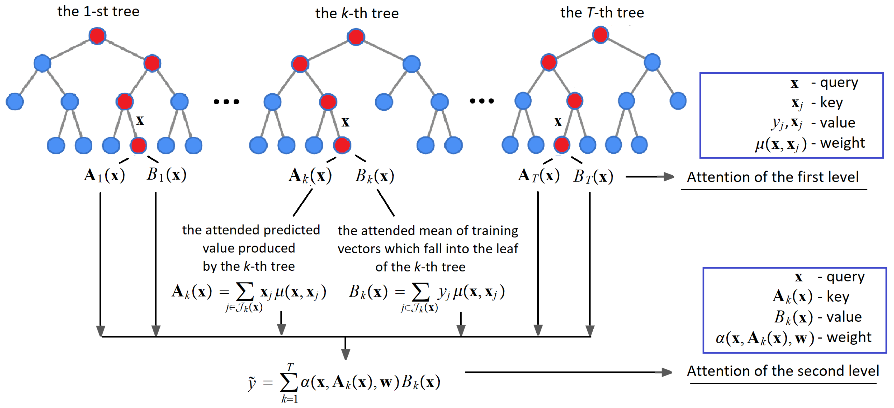
Let be the index set of examples which fall into the same leaf in the k-th tree as . One of the ways to construct the attention-based RF is to introduce the mean vector defined as the mean of the training vectors which fall into the same leaf as . However, this simple definition can be extended by incorporating the Nadaraya–Watson regression into the leaf. In this case, we can write
where is the attention weight in accordance with the Nadaraya–Watson kernel regression.
In fact, (4) can be regarded as the self-attention. The idea behind (4) is that we find the mean value of by assigning weights to training examples which fall into the corresponding leaf in accordance with their vicinity to the vector .
In the same way, we can define the mean value of regression outputs corresponding to examples falling into the same leaf as :
Expression (5) can be regarded as the attention. The idea behind (5) is to obtain the prediction provided by the corresponding leaf by using the standard attention mechanism or Nadaraya–Watson regression. In other words, we weigh predictions provided by the k-th leaf of a tree in accordance with the distance between the feature vector , which falls into the k-th leaf, and all the feature vectors which fall into the same leaf. It should be noted that the original regression tree provides the averaged prediction; i.e., it corresponds to the case when all are identical for all and equal to .
We suppose that the attention mechanisms used above are non-parametric. This implies that weights do not have trainable parameters. It is assumed that
The “leaf” attention introduced above can be regarded as the first-level attention in a hierarchy of the attention mechanisms. It characterizes how the feature vector fits the corresponding tree.
If we suppose that the whole RF consists of T decision trees, then, the set of , , in the framework of the attention mechanism, can be regarded as a set of keys for every , the set of , , can be regarded as a set of values. This implies that the final prediction of the RF can be computed by using the Nadaraya–Watson regression, namely,
Here, is the attention weight with the vector of trainable parameters which belong to a set so that they are assigned to each tree. The attention weight is defined by the distance between and . It is assumed due to properties of the attention weights in the Nadaraya–Watson regression that the following condition is valid:
The above “random forest” attention can be regarded as the second-level attention which assigns weights to trees in accordance with their impact on the RF prediction corresponding to .
The main idea behind the approach is to use the above attention mechanisms jointly. After substituting (4) and (5) into (7), we obtain
or
A scheme of the two-level attention is shown in Figure 1. It is observed from Figure 1 how the attention at the second level depends on the “leaf” attention at the first level.
In total, we obtain the trainable attention-based RF with parameters , which are defined by minimizing the expected loss function over the set of parameters, respectively, as follows:
The loss function can be rewritten as the following:
The optimal trainable parameters are computed depending on forms of the attention weights in the optimization problem (12). It should be noted that the problem (12) may be complex from the computation point of view. Therefore, one of our results is to propose such a form of the attention weights that reduces the problem (12) to a convex quadratic optimization problem, whose solution does not meet any difficulties.
It is important to point out that the additional sets of trainable parameters can be introduced into the definition of the attention weights . On the one hand, we obtain more flexible attention mechanisms in this case due to the parametrization of the training weights . On the other hand, many trainable parameters lead to the increasing complexity of the optimization problem (11) and the possible overfitting of the whole RF.
5. Modifications of the Two-Level Attention-Based Random Forest
Different configurations of LARF produce a set of models which depend on trainable parameters of the two-level attention and its implementation. A classification of models and their notations are shown in Table 1. In order to explain the classification, two subsets of the attention parameters should be considered:
- Parameters produced by the contamination probability distributions of Huber’s -contamination model in the form of the vector , whose length coincides with the number of trees.
- Parameters of contamination in the mixture of M in the Huber’s contamination models, which define the imprecision of the mixture model.
The following models can be constructed depending on trainable parameters and on using the “leaf” attention, i.e., the two-level attention mechanism:
- -ARF: The attention-based forest with learning as an attention parameter, but without the training vector , i.e., , , and without the “leaf” attention;
- w-ARF: The attention-based forest with the learning vector as attention parameters and without the “leaf” attention;
- -LARF: The attention-based forest with learning as an attention parameter, but without the training vector and with the “leaf” attention, i.e., by using the two-level attention mechanism;
- w-LARF: The attention-based forest with the learning vector as attention parameters and with the “leaf” attention, i.e., by using the two-level attention mechanism;
- -w-ARF: The attention-based forest with the learning vector and the parameter as attention parameters and without the “leaf” attention;
- -w-LARF: The attention-based forest with the learning vector and the parameter as attention parameters and with the “leaf” attention;
- -ARF: The attention-based forest with the learning parameters as attention parameters with , , and without the “leaf” attention;
- -LARF: The attention-based forest with the learning parameters as attention parameters with , , and with the “leaf” attention;
- -w-ARF: The attention-based forest with the learning vector and the parameters as attention parameters and without the “leaf” attention;
- -w-LARF: The attention-based forest with the learning vector and the parameters as attention parameters and with the “leaf” attention.
Models -ARF, -LARF, --ARF, and --LARF are not presented in Table 1 because they are special cases of models -ARF, -LARF, --ARF, and --LARF, respectively, by .
5.1. Huber’s Contamination Model and the Basic Two-Level Attention
In order to simplify the optimization problem (12) and to effectively solve it, we offer to represent the attention weights by using Huber’s -contamination model [14]. The idea to represent the attention weight by means of the -contamination model has been proposed in [8]. We use this idea to incorporate the -contamination model into the optimization problem (12) and to construct the first modifications of LARF.
Let us provide a brief introduction to Huber’s -contamination model. The model considers a set of probability distributions of the form . Here, is a discrete probability distribution contaminated by another probability distribution, denoted as , which can be arbitrary in the unit simplex having the dimension T. It is important to note that the distribution P depends on the feature vector , i.e., it is different for every vector , whereas the distribution R does not depend on . The contamination parameter controls the impact of the contamination probability distribution R on the distribution . Since the distribution R can be arbitrary, the set of the distributions F forms a subset of the unit simplex so that its size depends on the parameter . If , then the subset of distributions F is reduced to the single distribution . In case , the set of is the whole unit simplex.
Following the common definition of the attention weights through the softmax operation with the parameter , we propose to define each probability in as
This implies that the distribution characterizes how the feature vector is far from the vector in all trees of the RF. Let us suppose that the probability distribution R is the vector of the trainable parameters . The idea is to train the parameters to achieve the best accuracy of the RF. After substituting the softmax operation into the attention weight , we obtain:
One can observe from (13) that the attention weight is linearly dependent on the trainable parameters . It is important to note that the attention weight assigned to the k-th tree depends only on the k-th parameter , but not on other elements of the vector . The parameter is a tuning parameter determined by means of the standard validation procedure. It should be noted that elements of the vector are probabilities. Hence, we can write
This implies that the set is the unit simplex of the dimension T.
Let us return to the attention weight of the first level. The attention is non-parametric at the first level; therefore, the attention weight can be defined in the standard way by using the Gaussian kernel or the softmax operation with the parameter ; i.e., it can be expressed in this form:
Finally, we can rewrite the loss function (12) by taking into account the above definitions of the attention weights, as follows:
where
One can observe from the above that and do not depend on the parameters . Therefore, the objective function (16) jointly with the simple constraints or (14) is the standard quadratic optimization problem, which can be solved by means of many available efficient algorithms. The corresponding model is called -LARF. The notation means that trainable parameters are . The same model without “leaf” attention is denoted as -ARF. It coincides with the model -ABRF proposed in [8].
5.2. Models with the Trainable Contamination Parameter
One of the important contributions to the work, which makes the proposed model different from the model presented in [7,8], is the idea of learning the contamination parameter jointly with the parameters . However, this idea leads to a complex optimization problem, where gradient-based algorithms have to be used. In order to avoid using these algorithms and to tackle a simple optimization problem, we consider two ways. The first way is just to assign the same value to all parameters . Then, the optimization problem (16) can be rewritten as the following:
We have a simple quadratic optimization problem with one variable . Let us call the corresponding model as -LARF. The notation means that the trainable parameter is . The same model without the “leaf” attention is denoted as -ARF.
Another way is to introduce new variables , . Then, the optimization problem (16) can be rewritten in this form:
subject to
We again deal with the quadratic optimization problem with new optimization variables and linear constraints. The parameter takes a small value to avoid the case . The corresponding model is denoted as --LARF. The notation means that the trainable parameters are and . The same model without the “leaf” attention is denoted as --ARF.
5.3. Mixture of Contamination Models
Another important contribution is an attempt to search for an optimal value of the temperature parameter in (13) or in (17). We propose an approximate approach, which can significantly improve the model. Let us introduce a finite set of M values of the parameter . Here, M can be regarded as a tuning integer parameter which impacts the number of all training parameters. Large values of M may lead to a large number of training parameters and the corresponding overfitting. Small values of M may lead to an inexact approximation of .
Before considering how the optimization problem can be rewritten with allowance for the above information, we again return to the attention weight in (13) and represent it as follows:
where
We have a mixture of M contamination models with the different contamination parameters . It is obvious that the sum of new weights over is 1 because the sum of each over is also 1. Each forms a small simplex so that its center is defined by and its size is defined by . The corresponding sets of possible attention weights are depicted in Figure 2, where the unit simplex by includes small simplices corresponding to three () contamination models , , with different centers and different contamination parameters . The “mean” simplex of weights is depicted by using dashed sides. Parameters are optimized so that the attention weights will be located in the “mean” simplex.
Let us prove that the resulting “mean” model represents the -contamination model with the contamination parameter . We use to denote the probability distibution as follows:
Then, we can write
where
Suppose there is a probability distribution ; therefore, it holds
If we prove that the probability distribution Q exists, the resulting “mean” model is the -contamination model. Let us find sums of the left and the right sides of (28) over . Hence, we obtain
The introduced mixture of the contamination models can be regarded as a multi-head attention to some extent, where every “head” is produced by using a certain parameter .
Let us represent the softmax operation in (13) jointly with the factor as follows:
It can be observed from (30) that new parameters along with are introduced in the place of and , respectively. Term in (16) and (17) is replaced with the following terms:
where
Finally, we observed the following optimization problem:
subject to
Let us introduce new variables , , . Hence, we can write the optimization problem with the new variables as
subject to
We again face the quadratic optimization problem with linear constraints. The corresponding model will be denoted as --ARF or --LARF, depending on applying the “leaf” attention. The notation means that the trainable parameters are and . Additionally, we will use the same model, but with condition for all . The corresponding models are denoted as -ARF or -LARF.
6. Numerical Experiments
Let us introduce notations for different models of the attention-based RFs.
- RF (ERT): the original RF (the ERT) without applying attention mechanisms;
- ARF (LARF): the attention-based forest which has the following modifications: -ARF, -LARF, -w-ARF, and -w-LARF.
In all experiments, RFs as well as ERTs consist of 100 trees. To select the best tuning parameters in numerical experiments, a 3-fold cross-validation on the training set consisting of examples with 100 repetitions is performed. The search for the best parameter is carried out by considering all its values in a predefined grid. A cross-validation procedure is subsequently used to select their appropriate values. The testing set for computing the accuracy measures is comprised of examples. In order to obtain desirable estimates of the vectors and , all trees in the experiments are trained so that at least 10 examples fall into every leaf of a tree. Value 10 for the number of examples is taken for two reasons. On the one hand, we have to compute the mean vectors and and to obtain unbiased estimators. On the other hand, it is difficult to expect that a large number of examples will fall into every leaf by a small number of training examples. Therefore, our prior experiments have demonstrated that this parameter should be 10. We also use all features at each split of decision trees.
We do not consider models -ARF, -ARF, -LARF, and -LARF, because they can be regarded as special cases of the corresponding models M-ARF, --ARF, M-LARF, and --LARF when . The value of M is an integer tuning parameter, and it is tuned in the interval from 1 to 20. Set of the softmax operation parameters is defined as . In particular, if , then the set of consists of one element . The parameter of the first-level attention in the “leaf” is taken equal to 1.
Numerical results are presented in tables where the best results are shown in bold. The coefficient of determination denoted and the mean absolute error (MAE) are used for the regression evaluation. The greater value of the coefficient of determination and the smaller MAE we have, the better results we achieve.
The proposed approach is studied by applying datasets which are taken from open sources. The dataset Diabetes is downloaded from the R Packages; datasets Friedman 1, 2 and 3 are retrieved from the site: https://www.stat.berkeley.edu/~breiman/bagging.pdf (accessed on 20 April 2023); datasets Regression and Sparse are taken from package “Scikit-Learn”; datasets Wine Red, Boston Housing, Concrete, Yacht Hydrodynamics, Airfoil can be found in the UCI Machine Learning Repository [44]. These datasets with their numbers of features m and numbers of examples n are given in Table 2. A more detailed information can be found from the aforementioned data resources.
Values of the measure for several models, including RF, --ARF, --LARF, -ARF, and -LARF, are shown in Table 3. The results are obtained by training the RF. The optimal values of are also given in the table. It can be observed from Table 3 that --LARF outperforms all models for most datasets. Moreover, Table 3 shows that the two-level attention models (--LARF and -LARF) provide better results than models which do not use the “leaf” attention (--ARF and -ARF). It should be also noted that all attention-based models outperform the original RF. The same relationship between the models occurs for another accuracy measure (MAE). It is clearly shown in Table 4.
Another important question is how the attention-based models perform when the ERT is used. The corresponding values of and MAE are shown in Table 5 and Table 6, respectively. Table 5 also contains the optimal values . In contrast to the case of using the RF, it can be observed from the tables that -LARF outperforms --LARF for several models. It can be explained by reducing the accuracy due to a larger number of training parameters (parameters ) and overfitting for small datasets. It is also worth noting that models based on ERTs provide better results than models based on RFs. However, this improvement is not significant. This is observed in Table 7, where the best results are collected for models based on ERTs and RFs. Table 7 shows that the results are identical for several datasets, namely, for datasets Friedman 1, 2, 3, Concrete, and Yacht. If one is to apply the t-test to compare the values of obtained for two models, then, according to [45], the t-statistics is distributed in accordance with the Student distribution with the degrees of freedom (11 datasets). The obtained p-value is . We can conclude that the outperformance of the ERT is not statistically significant because .
We take the number of trees in RFs equal to 100, because our goal is to compare RFs and the proposed modifications of LARF with the same parameters of numerical experiments. We also study how values of depend on different numbers of decision trees for the considered datasets. The corresponding numerical results for the RF and the ERT are shown in Table 8 and Table 9, respectively, by 100, 400, 700, and 1000 trees. It can be observed in Table 8 and Table 9 that insignificantly increases with the number of trees. However, it is important to point out that the largest values of for RFs and ERTs obtained by do not exceed the values of for LARF modifications presented in Table 3, Table 4, Table 5 and Table 6.
It should be pointed out that the proposed models can be regarded as extensions of the attention-based RF (-ABRF) presented in [8]. Therefore, it is also worth comparing the two-level attention models with -ABRF. Table 10 shows the values of obtained by using -ABRF and the best values of the proposed models when the RF and the ERT are used.
If we compare the results presented in Table 10 by applying the t-tests in accordance with [45], then tests for the proposed models and -ABRF based on the RF and the ERT provide p-values equal to and , respectively. The tests demonstrate the clear outperformance of the proposed models in comparison with -ABRF.
It is obvious that the tuning parameters of the proposed modifications, for example, , are not optimal due to the validation procedure and due to the grid of values used in experiments. However, we can observe from the numerical results that the proposed modifications outperform RFs or -ABRF even with suboptimal values of the tuning parameters.
7. Conclusions
The new attention-based RF models proposed in the paper have supplemented the class attention models incorporated into machine learning models, differently from neural networks [7,8]. Moreover, the proposed models do not use gradient-based algorithms to learn attention parameters, and their training is based on solving the quadratic optimization problem with linear constraints. This peculiarity significantly simplifies the training process.
It is notable to point out that computing the attention weights in leaves of trees is a very simple task from the computational point of view. At the same time, this simple modification leads to the crucial improvement of the RF models. Numerical results with real data have demonstrated this improvement. This fact motivates us to continue developing attention-based modifications of machine learning models in different directions. First of all, the same approach can be applied to the gradient boosting machine [10]. The first successful attempt to use the attention mechanism in the gradient boosting machine with decision trees as base learners has been carried out in [7]. This attempt has confirmed that the boosting model can be improved by adding the attention component. The idea of the “leaf” attention and the optimization over parameters of kernels can be directly transferred to the gradient boosting machine. This is a direction for further research.
One of the important results presented in this paper is using a specific mixture of contamination models, which can be regarded as a variant of the well-known multi-head attention [16], where each “head” is defined by the kernel parameter. However, values of the parameter are selected in accordance with a predefined set. Therefore, the next direction is to consider randomized procedures to select the values of the parameter.
The proposed models consider only a single leaf of a tree for every example and implement the “leaf” attention in this leaf. However, they do not take into account neighbor leaves, which may also provide useful information for improving the models and should be studied.
It has been demonstrated in [8] that attention-based RFs allow us to interpret predictions by using the attention weights. The introduced two-level attention mechanisms may also improve the interpretability of RFs by taking into account additional factors.
Finally, we have developed the proposed modifications by using Huber’s -contamination model and the mixture of the models. Another notable problem is to consider different available statistical models [46] and their mixtures. A proper choice of the mixture components may significantly improve the whole attention-based RF.
Author Contributions
Conceptualization, L.U. and A.K.; methodology, L.U. and V.M.; software, A.K.; validation, V.M. and A.K.; formal analysis, A.K. and L.U.; investigation, A.K. and L.U.; resources, A.K. and V.M.; data curation, A.K. and V.M.; writing—original draft preparation, L.U.; writing—review and editing, A.K. and V.M.; supervision, L.U.; project administration, V.M.; funding acquisition, V.M. All authors have read and agreed to the published version of the manuscript.
Funding
The research is partially funded by the Ministry of Science and Higher Education of the Russian Federation as part of the World-class Research Center program: Advanced Digital Technologies (contract No. 075-15-2022-311 dated 20 April 2022).
Institutional Review Board Statement
Not applicable.
Informed Consent Statement
Not applicable.
Data Availability Statement
Not applicable.
Acknowledgments
The authors would like to express their appreciation to the anonymous referees whose very valuable comments have improved the paper.
Conflicts of Interest
The authors declare no conflict of interest.
References
- Chaudhari, S.; Mithal, V.; Polatkan, G.; Ramanath, R. An attentive survey of attention models. arXiv 2019, arXiv:1904.02874. [Google Scholar] [CrossRef]
- Correia, A.; Colombini, E. Attention, please! A survey of neural attention models in deep learning. arXiv 2021, arXiv:2103.16775. Available online: https://arxiv.org/abs/2103.16775 (accessed on 14 April 2023).
- Correia, A.; Colombini, E. Attention, please! A survey of neural attention models in deep learning. Artif. Intell. Rev. 2022, 55, 6037–6124. [Google Scholar] [CrossRef]
- Lin, T.; Wang, Y.; Liu, X.; Qiu, X. A Survey of Transformers. arXiv 2021, arXiv:2106.04554. [Google Scholar] [CrossRef]
- Niu, Z.; Zhong, G.; Yu, H. A review on the attention mechanism of deep learning. Neurocomputing 2021, 452, 48–62. [Google Scholar] [CrossRef]
- Breiman, L. Random forests. Mach. Learn. 2001, 45, 5–32. [Google Scholar] [CrossRef]
- Konstantinov, A.; Utkin, L.; Kirpichenko, S. AGBoost: Attention-based Modification of Gradient Boosting Machine. In Proceedings of the 31st Conference of Open Innovations Association (FRUCT), Helsinki, Finland, 27–29 April 2022; IEEE: Piscataway, NJ, USA, 2022; pp. 96–101. [Google Scholar]
- Utkin, L.; Konstantinov, A. Attention-based Random Forest and Contamination Model. Neural Netw. 2022, 154, 346–359. [Google Scholar] [CrossRef]
- Friedman, J. Greedy function approximation: A gradient boosting machine. Ann. Stat. 2001, 29, 1189–1232. [Google Scholar] [CrossRef]
- Friedman, J. Stochastic gradient boosting. Comput. Stat. Data Anal. 2002, 38, 367–378. [Google Scholar] [CrossRef]
- Zhang, A.; Lipton, Z.; Li, M.; Smola, A. Dive into Deep Learning. arXiv 2021, arXiv:2106.11342. [Google Scholar]
- Nadaraya, E. On estimating regression. Theory Probab. Appl. 1964, 9, 141–142. [Google Scholar] [CrossRef]
- Watson, G. Smooth regression analysis. Sankhya Indian J. Stat. Ser. A 1964, 26, 359–372. [Google Scholar]
- Huber, P. Robust Statistics; Wiley: New York, NY, USA, 1981. [Google Scholar]
- Utkin, L.; Konstantinov, A. Attention and Self-Attention in Random Forests. arXiv 2022, arXiv:2207.04293. [Google Scholar]
- Vaswani, A.; Shazeer, N.; Parmar, N.; Uszkoreit, J.; Jones, L.; Gomez, A.; Kaiser, L.; Polosukhin, I. Attention is all you need. In Proceedings of the Advances in Neural Information Processing Systems, Long Beach, CA, USA, 4–9 December 2017; pp. 5998–6008. [Google Scholar]
- Geurts, P.; Ernst, D.; Wehenkel, L. Extremely randomized trees. Mach. Learn. 2006, 63, 3–42. [Google Scholar] [CrossRef]
- Liu, F.; Huang, X.; Chen, Y.; Suykens, J. Random Features for Kernel Approximation: A Survey on Algorithms, Theory, and Beyond. arXiv 2021, arXiv:2004.11154v5. [Google Scholar] [CrossRef] [PubMed]
- Choromanski, K.; Likhosherstov, V.; Dohan, D.; Song, X.; Gane, A.; Sarlos, T.; Hawkins, P.; Davis, J.; Mohiuddin, A.; Kaiser, L.; et al. Rethinking Attention with Performers. In Proceedings of the 2021 International Conference on Learning Representations, Vienna, Austria, 3–7 May 2021; pp. 1–38. [Google Scholar]
- Choromanski, K.; Chen, H.; Lin, H.; Ma, Y.; Sehanobish, A.; Jain, D.; Ryoo, M.; Varley, J.; Zeng, A.; Likhosherstov, V.; et al. Hybrid Random Features. arXiv 2021, arXiv:2110.04367v2. [Google Scholar]
- Ma, X.; Kong, X.; Wang, S.; Zhou, C.; May, J.; Ma, H.; Zettlemoyer, L. Luna: Linear Unified Nested Attention. arXiv 2021, arXiv:2106.01540. [Google Scholar]
- Schlag, I.; Irie, K.; Schmidhuber, J. Linear transformers are secretly fast weight programmers. In Proceedings of the International Conference on Machine Learning 2021. PMLR, Virtual, 18–24 July 2021; pp. 9355–9366. [Google Scholar]
- Peng, H.; Pappas, N.; Yogatama, D.; Schwartz, R.; Smith, N.; Kong, L. Random Feature Attention. In Proceedings of the International Conference on Learning Representations (ICLR 2021), Vienna, Austria, 3–7 May 2021; pp. 1–19. [Google Scholar]
- Brauwers, G.; Frasincar, F. A General Survey on Attention Mechanisms in Deep Learning. arXiv 2022, arXiv:2203.14263. [Google Scholar] [CrossRef]
- Goncalves, T.; Rio-Torto, I.; Teixeira, L.; Cardoso, J. A survey on attention mechanisms for medical applications: Are we moving towards better algorithms? arXiv 2022, arXiv:2204.12406. [Google Scholar] [CrossRef]
- Santana, A.; Colombini, E. Neural Attention Models in Deep Learning: Survey and Taxonomy. arXiv 2021, arXiv:2112.05909. [Google Scholar]
- Soydaner, D. Attention Mechanism in Neural Networks: Where it Comes and Where it Goes. arXiv 2022, arXiv:2204.13154. [Google Scholar] [CrossRef]
- Xu, Y.; Wei, H.; Lin, M.; Deng, Y.; Sheng, K.; Zhang, M.; Tang, F.; Dong, W.; Huang, F.; Xu, C. Transformers in computational visual media: A survey. Comput. Vis. Media 2022, 8, 33–62. [Google Scholar] [CrossRef]
- Kim, H.; Kim, H.; Moon, H.; Ahn, H. A Weight-Adjusted Voting Algorithm for Ensemble of Classifiers. J. Korean Stat. Soc. 2011, 40, 437–449. [Google Scholar] [CrossRef]
- Ronao, C.; Cho, S.B. Random Forests with Weighted Voting for Anomalous Query Access Detection in Relational Databases. In Proceedings of the Artificial Intelligence and Soft Computing. ICAISC 2015, Zakopane, Poland, 14–18 June 2015; Lecture Notes in Computer Science. Springer: Cham, Switzerland, 2015; Volume 9120, pp. 36–48. [Google Scholar]
- Utkin, L.; Konstantinov, A.; Chukanov, V.; Meldo, A. A New Adaptive Weighted Deep Forest and its Modifications. Int. J. Inf. Technol. Decis. 2020, 19, 963–986. [Google Scholar] [CrossRef]
- Winham, S.; Freimuth, R.; Biernacka, J. A Weighted Random Forests Approach to Improve Predictive Performance. Stat. Anal. Data Min. 2013, 6, 496–505. [Google Scholar] [CrossRef]
- Xuan, S.; Liu, G.; Li, Z. Refined Weighted Random Forest and Its Application to Credit Card Fraud Detection. In Proceedings of the Computational Data and Social Networks, Shanghai, China, 18–20 December 2018; Springer International Publishing: Cham, Switzerland, 2018; pp. 343–355. [Google Scholar]
- Zhang, X.; Wang, M. Weighted Random Forest Algorithm Based on Bayesian Algorithm. In Journal of Physics: Conference Series; IOP Publishing: Bristol, UK, 2021; Volume 1924, pp. 1–6. [Google Scholar]
- Abellan, J.; Moral, S. Building Classification Trees Using th Building Classification Trees Using the Total Uncertainty Criterion. Int. J. Intell. Syst. 2003, 18, 1215–1225. [Google Scholar] [CrossRef]
- Abellan, J.; Mantas, C.; Castellano, J. A Random Forest approach using imprecise probabilities. Knowl.-Based Syst. 2017, 134, 72–84. [Google Scholar] [CrossRef]
- Abellan, J.; Mantas, C.; Castellano, J.; Moral-Garcia, S. Increasing diversity in random forest learning algorithm via imprecise probabilities. Expert Syst. Appl. 2018, 97, 228–243. [Google Scholar] [CrossRef]
- Mantas, C.; Abellan, J. Analysis and extension of decision trees based on imprecise probabilities: Application on noisy data. Expert Syst. Appl. 2014, 41, 2514–2525. [Google Scholar] [CrossRef]
- Moral-Garcia, S.; Mantas, C.; Castellano, J.; Benitez, M.; Abellan, J. Bagging of credal decision trees for imprecise classification. Expert Syst. Appl. 2020, 141, 1–9. [Google Scholar] [CrossRef]
- Utkin, L.; Wiencierz, A. An imprecise boosting-like approach to regression. In Proceedings of the ISIPTA ’13, Proceedings of the Eighth International Symposium on Imprecise Probability: Theories and Applications, Compiegne, France, 2–5 July 2013; Cozman, F., Denoeux, T., Destercke, S., Seidfenfeld, T., Eds.; SIPTA: Compiegne, France, 2013; pp. 345–354. [Google Scholar]
- Utkin, L.; Kovalev, M.; Coolen, F. Imprecise weighted extensions of random forests for classification and regression. Appl. Soft Comput. 2020, 92, 1–14. [Google Scholar] [CrossRef]
- Bahdanau, D.; Cho, K.; Bengio, Y. Neural machine translation by jointly learning to align and translate. arXiv 2014, arXiv:1409.0473. [Google Scholar]
- Luong, T.; Pham, H.; Manning, C. Effective approaches to attention-based neural machine translation. In Proceedings of the 2015 Conference on Empirical Methods in Natural Language Processing, Lisbon, Portugal, 17–21 September 2015; The Association for Computational Linguistics: NewYork, NY, USA, 2015; pp. 1412–1421. [Google Scholar]
- Dua, D.; Graff, C. UCI Machine Learning Repository. 2017. Available online: http://archive.ics.uci.edu/ml (accessed on 20 April 2023).
- Demsar, J. Statistical comparisons of classifiers over multiple data sets. J. Mach. Learn. Res. 2006, 7, 1–30. [Google Scholar]
- Walley, P. Statistical Reasoning with Imprecise Probabilities; Chapman and Hall: London, UK, 1991. [Google Scholar]
Figure 1.
A scheme of the proposed two-level hierarchical attention model applied to the RF.

Figure 2.
The unit simplex of possible attention weights, which includes small simplices corresponding to three contamination models with different centers and different contamination parameters and the “mean” simplex (with dashed sides), which defines the set of the final attention weights.
Figure 2.
The unit simplex of possible attention weights, which includes small simplices corresponding to three contamination models with different centers and different contamination parameters and the “mean” simplex (with dashed sides), which defines the set of the final attention weights.


Table 1.
Classification of the attention-based RF models proposed and studied in this paper.
| Tuning | Trainable | |||
|---|---|---|---|---|
| Fixed | Trainable | Fixed | Trainable | |
| Without the “leaf” attention | - | -ARF | -ARF | --ARF |
| With the “leaf” attention | - | -LARF | -LARF | --LARF |
Table 2.
A brief introduction about the regression data sets.
| Data Set | Abbreviation | m | n |
|---|---|---|---|
| Diabetes | Diabetes | 10 | 442 |
| Friedman 1 | Friedman 1 | 10 | 100 |
| Friedman 2 | Friedman 2 | 4 | 100 |
| Friedman 3 | Friedman 3 | 4 | 100 |
| Scikit-Learn Regression | Regression | 100 | 100 |
| Scikit-Learn Sparse Uncorrelated | Sparse | 10 | 100 |
| UCI Wine red | Wine | 11 | 1599 |
| UCI Boston Housing | Boston | 13 | 506 |
| UCI Concrete | Concrete | 8 | 1030 |
| UCI Yacht Hydrodynamics | Yacht | 6 | 308 |
| UCI Airfoil | Airfoil | 5 | 1503 |
Table 3.
Values of for comparison of models based on the RF.
| Data Set | RF | -w-ARF | -w-LARF | -ARF | -LARF | |
|---|---|---|---|---|---|---|
| Diabetes | . | |||||
| Friedman 1 | 1 | . | ||||
| Friedman 2 | 1 | . | ||||
| Friedman 3 | 1 | . | ||||
| Airfoil | 100 | . | ||||
| Boston | 1 | . | ||||
| Concrete | 10 | . | . | |||
| Wine | 1 | . | ||||
| Yacht | . | |||||
| Regression | . | |||||
| Sparse | 1 | . |
The best obtained results on each dataset are shown in bold.
Table 4.
Values of MAE for comparison of models based on the RF.
| Data Set | RF | -w-ARF | -w-LARF | -ARF | -LARF |
|---|---|---|---|---|---|
| Diabetes | . | ||||
| Friedman 1 | . | ||||
| Friedman 2 | . | ||||
| Friedman 3 | . | ||||
| Airfoil | . | ||||
| Boston | . | ||||
| Concrete | . | ||||
| Wine | . | ||||
| Yacht | . | ||||
| Regression | . | ||||
| Sparse | . |
The best obtained results on each dataset are shown in bold.
Table 5.
Values of for comparison of models based on the ERT.
| Data Set | ERT | -w-ARF | -w-LARF | -ARF | -LARF | |
|---|---|---|---|---|---|---|
| Diabetes | . | |||||
| Friedman 1 | 1 | . | ||||
| Friedman 2 | 10 | . | ||||
| Friedman 3 | 1 | . | ||||
| Airfoil | 100 | . | ||||
| Boston | 10 | . | ||||
| Concrete | 10 | . | ||||
| Wine | 1 | . | ||||
| Yacht | 1 | . | . | |||
| Regression | . | |||||
| Sparse | 1 | . |
The best obtained results on each dataset are shown in bold.
Table 6.
Values of MAE for comparison of models based on the ERT.
| Data Set | ERT | w-ARF | w-LARF | -ARF | -LARF |
|---|---|---|---|---|---|
| Diabetes | . | ||||
| Friedman 1 | . | ||||
| Friedman 2 | . | ||||
| Friedman 3 | . | ||||
| Airfoil | . | ||||
| Boston | . | ||||
| Concrete | . | ||||
| Wine | . | ||||
| Yacht | . | ||||
| Regression | . | ||||
| Sparse | . |
The best obtained results on each dataset are shown in bold.
Table 7.
Comparison of the best results provided by models based on RFs and ERTs.
| Data Set | RF | ERT |
|---|---|---|
| Diabetes | . | |
| Friedman 1 | . | . |
| Friedman 2 | . | . |
| Friedman 3 | . | . |
| Airfoil | . | |
| Boston | . | |
| Concrete | . | . |
| Wine | . | |
| Yacht | . | . |
| Regression | . | |
| Sparse | . |
The best obtained results on each dataset are shown in bold.
Table 8.
Values of for comparison of RFs by different numbers of decision trees.
| Data Set | Numbers of Trees | |||
|---|---|---|---|---|
| 100 | 400 | 700 | 1000 | |
| Diabetes | ||||
| Friedman 1 | ||||
| Friedman 2 | ||||
| Friedman 3 | ||||
| Airfoil | ||||
| Boston | ||||
| Concrete | ||||
| Wine | ||||
| Yacht | ||||
| Regression | ||||
| Sparse | ||||
Table 9.
Values of for comparison of ERTs by different numbers of decision trees.
| Data Set | Numbers of Trees | |||
|---|---|---|---|---|
| 100 | 400 | 700 | 1000 | |
| Diabetes | ||||
| Friedman 1 | ||||
| Friedman 2 | ||||
| Friedman 3 | ||||
| Airfoil | ||||
| Boston | ||||
| Concrete | ||||
| Wine | ||||
| Yacht | ||||
| Regression | ||||
| Sparse | ||||
Table 10.
Comparison of -ABRF and the proposed models by using the measure when RFs and ERTs are the basis.
Table 10.
Comparison of -ABRF and the proposed models by using the measure when RFs and ERTs are the basis.
| Data Set | RF | ERT | ||
|---|---|---|---|---|
| -ABRF | LARF | -ABRF | LARF | |
| Diabetes | ||||
| Friedman 1 | ||||
| Friedman 2 | ||||
| Friedman 3 | ||||
| Airfoil | ||||
| Boston | ||||
| Concrete | ||||
| Wine | ||||
| Yacht | ||||
| Regression | ||||
| Sparse | ||||
The best obtained results on each dataset are shown in bold.
Disclaimer/Publisher’s Note: The statements, opinions and data contained in all publications are solely those of the individual author(s) and contributor(s) and not of MDPI and/or the editor(s). MDPI and/or the editor(s) disclaim responsibility for any injury to people or property resulting from any ideas, methods, instructions or products referred to in the content. |
© 2023 by the authors. Licensee MDPI, Basel, Switzerland. This article is an open access article distributed under the terms and conditions of the Creative Commons Attribution (CC BY) license (https://creativecommons.org/licenses/by/4.0/).
Share and Cite
MDPI and ACS Style
Konstantinov, A.; Utkin, L.; Muliukha, V. LARF: Two-Level Attention-Based Random Forests with a Mixture of Contamination Models. Informatics 2023, 10, 40. https://doi.org/10.3390/informatics10020040
AMA Style
Konstantinov A, Utkin L, Muliukha V. LARF: Two-Level Attention-Based Random Forests with a Mixture of Contamination Models. Informatics. 2023; 10(2):40. https://doi.org/10.3390/informatics10020040
Chicago/Turabian StyleKonstantinov, Andrei, Lev Utkin, and Vladimir Muliukha. 2023. "LARF: Two-Level Attention-Based Random Forests with a Mixture of Contamination Models" Informatics 10, no. 2: 40. https://doi.org/10.3390/informatics10020040
Note that from the first issue of 2016, this journal uses article numbers instead of page numbers. See further details here.