
An IoT-Fog-Cloud Integrated Framework for Real-Time Remote Cardiovascular Disease Diagnosis
 ,
,
Abstract
:1. Introduction
1.1. Research Gap and Research Questions
1.2. Motivations and Objective
1.3. Contributions
- Identifying and assessing earlier work in heart disease diagnoses in real time from abroad;
- Examining the work using many measures and an integrated heart disease dataset;
- Constructing a simple, automated, EML- and EDL-based heart patient diagnosis system;
- Using a variety of IoT-Fog-Cloud frameworks and simulators to perform the most accurate predictive analytics;
- Addressing the results and comparing them with the results of earlier studies,
- Finding crucial areas where this can be combined with Fog computing studies to promote the application of these methods.
1.4. Paper Organization
2. Existing Works
3. Preliminaries
3.1. Dataset Description, Preparation, and Preprocessing
3.2. Materials and Methods
4. Proposed Work: FRIEND
4.1. Architecture of FRIEND
4.2. Design of FRIEND
4.2.1. Android Application and Experimental Setup
4.2.2. Implementation
4.3. Working of FRIEND
| Algorithm 1: Detailed working of FRIEND |
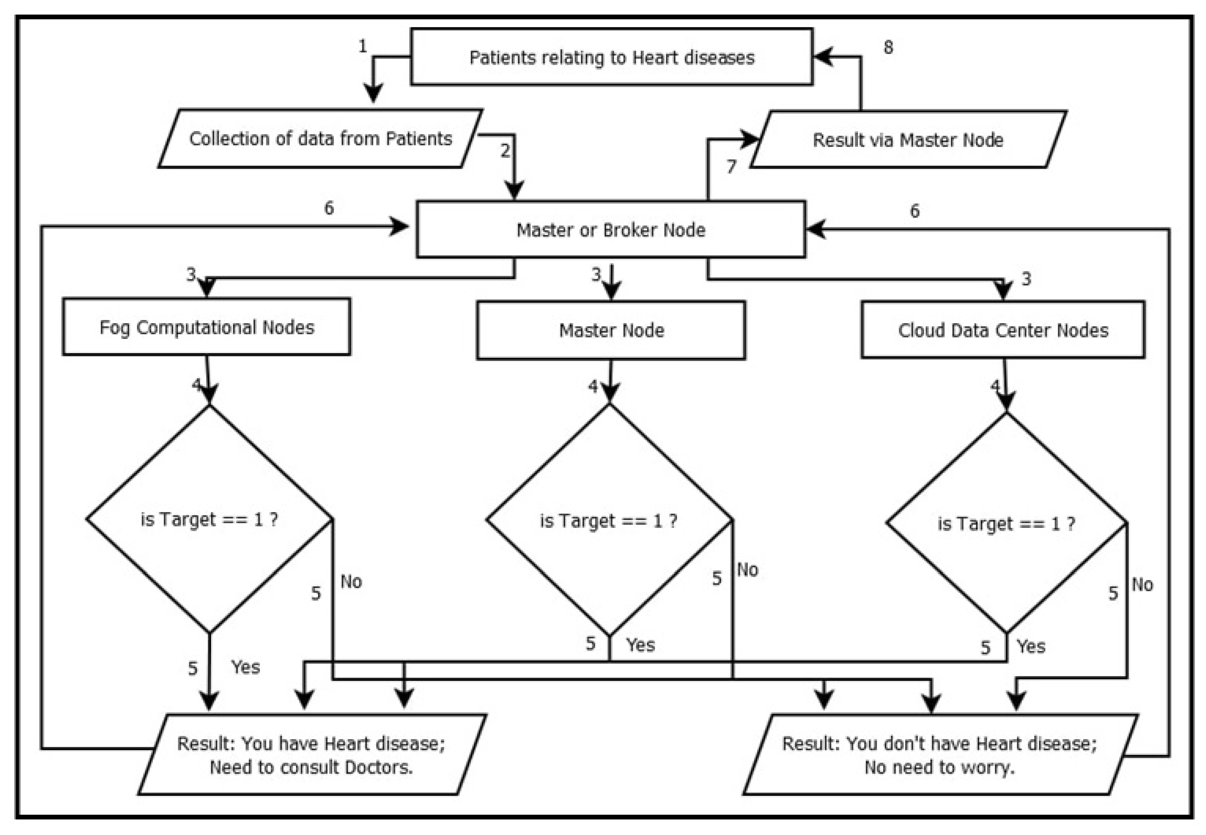
| Notations: PAD: Patients’ data GTD: Gateway device ITD: IoT device ATR: Attribute FWN: Fog computational node CCN: Cloud Data center node MBP: Master/broker node RES: Result Input: Patients’ data, PADi = {PAD1, PAD2, PAD3. . . } Gateway devices, GTDi = {GTD1, GTD2, GTD3. . . } IoT devices, ITDi = {ITD1, ITD2, ITD3. . . } Attributes, ATRi = {ATR1 for age, ATR2 for sex, ATR3 for chest pain type, ATR4 for blood pressure, ATR5 for smoking years, ATR6 for fasting blood sugar level, ATR7 for diabetes history, ATR8 for family history coronary, ATR9 for ECG, ATR10 for pulse rate, ATR11 for target} Fog computational nodes, FWNi = {FWN1, FWN2, FWN3. . . } Output: Results, RESi = {RES0 when value of target is 0, RES1 when value of target is 1} Steps of Algorithm: Obtain ATR3, ATR4, ATR6, ATR9 and ATR10 using ITDi. Submit PADi obtained using ITDi adding ATR1, ATR2, ATR5, ATR7, and ATR8 to MBP using GTDi. if MBP = = available (), then if target = = 1, then return RES1 else return RES0 end if end if if FWNi = = available (), then if target = = 1, then return RES1 else return RES0 end if end if if CCN = = available () then if target = = 1 then return RES1 else return RES0 end if end if Return RESi to MBP. Transfer RESi to the corresponding GTDi. |
| Algorithm 2: Pseudocode of EDL algorithm employed in FRIEND |
| Notations: S: Samples B: Bagging algorithm M: ML algorithm D: DL algorithm E: EL algorithm P: Total number of iterations R: Result Input: Training samples, Si = {S1, S2, S3. . . } Bagging algorithms, Bi = {B1, B2, B3. . . } ML algorithms, Mi = {M1, M2, M3. . . } DL algorithms, Di = {D1, D2, D3. . . } EL algorithms, Ei = {E1 for weighted averaging, E2 for soft voting, E3 for hard voting} Output: Results, R Steps of Algorithm: Begin for i = 1 to P do Obtain Si if Algorithm == Di then Training Di on Si Bootstrap Di using Bi else Training Mi on Si end if end for Get R, Applying Ei Assign R to the nearest {0,1} End. |
5. Experimental Results and Discussion
5.1. Analysis of Results Based on Performance Parameters
5.2. Analysis of Results Based on Network Parameters
5.3. Comparative Analysis
6. Conclusions
Author Contributions
Funding
Institutional Review Board Statement
Informed Consent Statement
Data Availability Statement
Conflicts of Interest
References
- DuBravac, S.; Ratti, C. The internet of things: Evolution or revolution? AIG White Pap. 2015, 1, 1–22. [Google Scholar]
- Lakhan, A.; Mohammed, M.A.; Kozlov, S.; Rodrigues, J.J. Mobile-fog-cloud assisted deep reinforcement learning and blockchain-enable IoMT system for healthcare workflows. Trans. Emerg. Telecommun. Technol. 2021, e4363. [Google Scholar] [CrossRef]
- Pati, A.; Parhi, M.; Pattanayak, B.K. IDMS: An Integrated Decision Making System for Heart Disease Prediction. In Proceedings of the 2021 1st Odisha International Conference on Electrical Power Engineering, Communication and Computing. Technology (ODICON), Bhubaneswar, India, 8–9 January 2021; pp. 1–6. [Google Scholar]
- Gupta, R.; Mohan, I.; Narula, J. Trends in coronary heart disease epidemiology in India. Ann. Glob. Health 2016, 82, 307–315. [Google Scholar] [PubMed]
- Shukla, S.; Thakur, S.; Hussain, S.; Breslin, J.G.; Jameel, S.M. Identification and Authentication in Healthcare Internet-of-Things Using Integrated Fog Computing Based Blockchain Model. Internet Things 2021, 15, 100422. [Google Scholar] [CrossRef]
- Pati, A.; Parhi, M.; Pattanayak, B.K. IADP: An integrated approach for diabetes prediction using classification techniques. In Proceedings of the Advances in Distributed Computing and Machine Learning 2021, Singapore, 15–16 January 2021; pp. 287–298. [Google Scholar] [CrossRef]
- Islam, S.R.; Kwak, D.; Kabir, M.H.; Hossain, M.; Kwak, K.S. The internet of things for health care: A comprehensive survey. IEEE Access 2015, 3, 678–708. [Google Scholar] [CrossRef]
- Rahmani, A.M.; Gia, T.N.; Negash, B.; Anzanpour, A.; Azimi, I.; Jiang, M.; Liljeberg, P. Exploiting smart e-Health gateways at the edge of healthcare Internet-of-Things: A fog computing approach. Futur. Gener. Comput. Syst. 2018, 78, 641–658. [Google Scholar] [CrossRef]
- Mutlag, A.A.; Ghani, M.K.A.; Mohammed, M.A.; Lakhan, A.; Mohd, O.; Abdulkareem, K.H.; Garcia-Zapirain, B. Multi-Agent Systems in Fog–Cloud Computing for Critical Healthcare Task Management Model (CHTM) Used for ECG Monitoring. Sensors 2021, 21, 6923. [Google Scholar] [CrossRef]
- Gill, S.S.; Arya, R.C.; Wander, G.S.; Buyya, R. August Fog-based smart healthcare as a big data cloud service for heart patients using IoT. In Proceedings of the International Conference on Intelligent Data Communication Technologies and Internet of Things, Coimbatore, India, 7–8 August 2018; Springer: Berlin/Heidelberg, Germany, 2018; pp. 1376–1383. [Google Scholar]
- Priyadarshini, R.; Barik, R.K.; Dubey, H. Deepfog: Fog computing-based deep neural architecture for prediction of stress types, diabetes and hypertension attacks. Computation 2018, 6, 62. [Google Scholar] [CrossRef]
- Caliskan, A.; Yuksel, M.E. Classification of coronary artery disease data sets by using a deep neural network. EuroBiotech J. 2017, 1, 271–277. [Google Scholar] [CrossRef]
- Choi, E.; Bahadori, M.T.; Song, L.; Stewart, W.F.; Sun, J. August GRAM: Graph-based attention model for healthcare representation learning. In Proceedings of the 23rd ACM SIGKDD International Conference on Knowledge Discovery and Data Mining, Halifax, NS, Canada, 13–17 August 2017; pp. 787–795. [Google Scholar]
- Ali, S.; Ghazal, M. April Real-time heart attack mobile detection service (RHAMDS): An IoT use case for software defined networks. In Proceedings of the 2017 IEEE 30th Canadian Conference on Electrical and Computer Engineering (CCECE), Windsor, ON, Canada, 30 April–3 May 2017; pp. 1–6. [Google Scholar]
- Gupta, S. Classification of Heart Disease Hungarian Data Using Entropy, Knnga Based Classifier and Optimizer. Int. J. Eng. Technol. 2018, 7, 292–296. [Google Scholar] [CrossRef] [Green Version]
- Mustafa, J.; Awan, A.A.; Khalid, M.S.; Nisar, S. Ensemble approach for developing a smart heart disease prediction system using classification algorithms. Res. Rep. Clin. Cardiol. 2018, 9, 33. [Google Scholar]
- Zhenya, Q.; Zhang, Z. A hybrid cost sensitive ensemble for heart disease prediction. BMC Med. Inform. Decis. Mak. 2021, 21, 1–18. [Google Scholar] [CrossRef] [PubMed]
- Ali, F.; El-Sappagh, S.; Islam, S.R.; Kwak, D.; Ali, A.; Imran, M.; Kwak, K.-S. A smart healthcare monitoring system for heart disease prediction based on ensemble deep learning and feature fusion. Inf. Fusion 2020, 63, 208–222. [Google Scholar] [CrossRef]
- Moghadas, E.; Rezazadeh, J.; Farahbakhsh, R. An IoT patient monitoring based on fog computing and data mining: Cardiac arrhythmia use case. Internet Things 2020, 11, 100251. [Google Scholar]
- Baccouche, A.; Garcia-Zapirain, B.; Olea, C.C.; Elmaghraby, A. Ensemble Deep Learning Models for Heart Disease Classification: A Case Study from Mexico. Information 2020, 11, 207. [Google Scholar] [CrossRef]
- Sun, L.; Yu, Q.; Peng, D.; Subramani, S.; Wang, X. FogMed: A Fog-based Framework for Disease Prognosis Based Medical Sensor Data Streams. Comput. Mater. Contin. 2020, 66, 603–619. [Google Scholar] [CrossRef]
- Tuli, S.; Basumatary, N.; Gill, S.S.; Kahani, M.; Arya, R.C.; Wander, G.S.; Buyya, R. HealthFog: An ensemble deep learning based Smart Healthcare System for Automatic Diagnosis of Heart Diseases in integrated IoT and fog computing environments. Future Gener. Comput. Syst. 2020, 104, 187–200. [Google Scholar]
- Sharma, S.; Parmar, M. Heart diseases prediction using deep learning neural network model. Int. J. Innov. Technol. Explor. Eng. 2020, 9, 124–137. [Google Scholar] [CrossRef]
- Uddin, M.N.; Halder, R.K. An ensemble method based multilayer dynamic system to predict cardiovascular disease using machine learning approach. Inform. Med. Unlocked 2021, 24, 100584. [Google Scholar] [CrossRef]
- Heart Disease Data Set. UCI Machine Learning Repository. Available online: https://archive.ics.uci.edu/ml/datasets/heart+disease (accessed on 4 December 2020).
- Gupta, H.; Vahid Dastjerdi, A.; Ghosh, S.K.; Buyya, R. iFogSim: A toolkit for modeling and simulation of resource management techniques in the Internet of Things, Edge and Fog computing environments. Softw. Pract. Exp. 2017, 47, 1275–1296. [Google Scholar] [CrossRef]
- Tuli, S.; Mahmud, R.; Tuli, S.; Buyya, R. Fogbus: A blockchain-based lightweight framework for edge and fog computing. J. Syst. Softw. 2019, 154, 22–36. [Google Scholar]
- Narula, S.; Jain, A. February Cloud computing security: Amazon web service. In Proceedings of the 2015 Fifth International Conference on Advanced Computing & Communication Technologies, Rohtak, India, 21–22 February 2015; pp. 501–505. [Google Scholar]
- Vecchiola, C.; Chu, X.; Buyya, R. Aneka: A software platform for NET-based cloud computing. High Speed Large Scale Sci. Comput. 2009, 18, 267–295. [Google Scholar]
- Qalaja, E.K.; Abu Al-Haija, Q.; Tareef, A.; Al-Nabhan, M.M. Inclusive Study of Fake News Detection for COVID-19 with New Dataset using Supervised Learning Algorithms. Int. J. Adv. Comput. Sci. Appl. 2022, 13, 1–22. [Google Scholar] [CrossRef]
- Hasan, T.T.; Jasim, M.H.; Hashim, I.A. Heart disease diagnosis system based on multi-layer perceptron neural network and support vector machine. Int. J. Curr. Eng. Technol. 2017, 77, 2277–4106. [Google Scholar]
- Yan, H.; Jiang, Y.; Zheng, J.; Peng, C.; Li, Q. A multilayer perceptron-based medical decision support system for heart disease diagnosis. Expert Syst. Appl. 2006, 30, 272–281. [Google Scholar] [CrossRef]
- Livieris, I.E.; Pintelas, E.; Stavroyiannis, S.; Pintelas, P. Ensemble deep learning models for forecasting cryptocurrency time-series. Algorithms 2020, 13, 121. [Google Scholar] [CrossRef]
- Explore MIT App Inventor. MIT App Inventor. Available online: https://appinventor.mit.edu/ (accessed on 24 July 2020).
- Ahmad, A.A.-S.; Andras, P. Scalability analysis comparisons of cloud-based software services. J. Cloud Comput. 2019, 8, 10. [Google Scholar] [CrossRef]
- Alnabhan, M.; Habboush, A.K.; Abu Al-Haija, Q.; Mohanty, A.K.; Pattnaik, S.; Pattanayak, B.K. Hyper-Tuned CNN Using EVO Technique for Efficient Biomedical Image Classification. Mob. Inf. Syst. 2022, 2022, 2123662. [Google Scholar] [CrossRef]


| Work | Materials and Methods | Dataset Used | Evaluative Measures | Findings |
|---|---|---|---|---|
| [12] | Proposed DNN classifier for categorizing coronary artery disease | Switzerland, LongBeach, Hungarian, and Cleveland HDDs | Accuracy, sensitivity, and specificity | The suggested classifier is affordable and readily available |
| [13] | Introduced RNN-based model termed GRAM, i.e., graph-based attention model | Datasets from PAMF and MIMIC–III | Accuracy, data needs, and interpretability | The proposed GRAM approach significantly improves performance on low-frequency diseases and small datasets |
| [14] | Introduced RHAMDS, i.e., real-time heart attack mobile detection service | Real-time dataset | Voice and gesture control | The planned RHAMDS reduces and prevents automobile crashes by identifying drivers who are having heart attacks |
| [15] | Introduced a hybrid technique combining KNN and GA approaches | Hungarian HDD | Accuracy | The suggested paradigm yields outcomes that are more precise and effective |
| [16] | Proposed an ensemble model with SVM, ANN, NB, RA, and RF to investigate and forecast the recurrence of cardiovascular illness | Hungarian and Cleveland HDDs | Accuracy, precision, F-M, ROC, RMSE, and kappa statistics | This ensemble technique achieves both high readability and predictive accuracy |
| [17] | Proposed a 5-classifier-based affordable ensemble technique to enhance the detection of heart disease | Cleveland, Statlog, and Hungarian HDDs | Precision, AUC specificity, E, recall, MC, and G-mean | This ensemble method outperforms others and offers a possible alternative |
| [18] | Feature fusion and EDL are used to predict cardiovascular disease | Cleveland and Hungarian HDDs | Accuracy, recall, MAE, precision, F-measure, and RMSE | This ensemble strategy leads to more accurate heart disease predictions |
| [19] | Presented a method for remote monitoring of a patient utilizing an Arduino board and an AD8232 sensor module | Tele ECG | Accuracy and macro-F1 | The KNN classifier-based system is ideal for both classification and validation |
| [20] | Proposed CNN-based EL framework for heart disease data classification | Mexico’s Medica Dataset | Accuracy and F1-score | The suggested approach classifies imbalanced HDDs more accurately |
| [21] | Proposed FogMed framework for heart disease prediction | ECG dataset | Accuracy and time efficiency | The proposed framework outperforms existing CC methods. |
| [22] | Introduced EDL-based HealthFog for automatic cardiac patient analysis in FC and IoT | Cleveland HDD | Accuracy and network parameters | HealthFog detects cardiac patients remotely in real-time |
| [23] | Introduced NN-based DL for cardiovascular disease prediction | Cleveland HDD | Accuracy | This DNN technology outperforms previous methods |
| [24] | IGAE, GAIN, CAE, lasso, and ETs were used to introduce MLDS, an EM-based multilayer dynamic system | Realistic dataset from Kaggle | Accuracy, precision, ROC, and AUC | Cardiovascular disease can be accurately predicted by the suggested MLDS |
| Dataset Used | Quantity of Attributes | Quantity of Instances |
|---|---|---|
| IHDD | 76 (11 considered in this Work) | 303 (Cleveland HDD), 123 (Switzerland HDD), 294 (Hungarian HDD), and 200 (Long Beach VA HDD) |
| Sl. | Attributes | Meaning | Values |
|---|---|---|---|
| 1 | Age | Patient’s age in years | A number value (between 29 and 79) |
| 2 | Sex | Patient’s gender | 0: female; 1: male |
| 3 | Chest pain | Type of chest pains | 1: typical angina; 2: atypical angina; 3: non-anginal pain; 4: asymptomatic |
| 4 | Blood pressure | Resting blood pressure level (in mm Hg on admission to the hospital) | A numeric value (between 94 and 200) |
| 5 | Smoking years | Years that a person has smoked | A numeric value (between 5 and 45) |
| 6 | Fasting blood sugar | Level of fasting blood sugar | 0: false, if FBS is less than or equal to 120 mg/dL; 1: true, if FBS is greater than 120 mg/dL |
| 7 | Diabetes history | Prior diabetic history | 0: no history of diabetes; 1: history of diabetes |
| 8 | Family cornory history | Coronary disease in the family | 0: no; 1: yes |
| 9 | Rest ECG | Electrocardiographic readings while at rest | 0: normal; 1: having ST-T wave abnormality (T wave inversions and/or ST elevation or depression of >0.05 mV); 2: showing probable or definite left ventricular hypertrophy by Estes’ criteria |
| 10 | Pulse rate | Reached maximum heart rate | A numeric value (between 71 and 202) |
| 11 | Target | Heart disease diagnosis | 0: for <50% diameter narrowing; 1: >50% diameter narrowing |
| Sl. | Age | Sex | Chest Pain | Blood Pressure | Smoking Years | Fasting Blood Sugar | Diabetes History | Family Cornory History | Rest ECG | Pulse Rate | Target |
|---|---|---|---|---|---|---|---|---|---|---|---|
| 0 | 63 | 1 | 1 | 145.0 | 20.0 | 1.0 | 1.0 | 1.0 | 2.0 | 150.0 | 0 |
| 1 | 67 | 1 | 4 | 160.0 | 40.0 | 0.0 | 1.0 | 1.0 | 2.0 | 108.0 | 0 |
| 2 | 67 | 1 | 4 | 120.0 | 35.0 | 0.0 | 1.0 | 1.0 | 2.0 | 129.0 | 0 |
| 3 | 37 | 1 | 3 | 130.0 | 0.0 | 0.0 | 1.0 | 1.0 | 0.0 | 187.0 | 0 |
| 4 | 41 | 0 | 2 | 130.0 | 0.0 | 0.0 | 1.0 | 1.0 | 2.0 | 172.0 | 0 |
| 5 | 56 | 1 | 2 | 120.0 | 20.0 | 0.0 | 1.0 | 1.0 | 0.0 | 178.0 | 0 |
| 6 | 62 | 0 | 4 | 140.0 | 0.0 | 0.0 | 1.0 | 1.0 | 2.0 | 160.0 | 1 |
| 7 | 57 | 0 | 4 | 120.0 | 0.0 | 0.0 | 1.0 | 1.0 | 0.0 | 163.0 | 0 |
| 8 | 63 | 1 | 4 | 130.0 | 0.0 | 0.0 | 1.0 | 0.0 | 2.0 | 147.0 | 0 |
| 9 | 53 | 1 | 4 | 140.0 | 25.0 | 1.0 | 1.0 | 1.0 | 2.0 | 155.0 | 0 |
| Dataset | Model | Input Layers Numbers | Hidden Layers Numbers | Output Layers Numbers | Optimizer Used | Learning Rate | Input Layers AF | Hidden Layers AF | Output Layers AF |
|---|---|---|---|---|---|---|---|---|---|
| IHDD | DNN | 10 | 3 | 2 | Adam | 0.12 | ReLU | ReLU | Sigmoid |
| ML Approaches | Recorded Performance Measures (in %) | |||||||||||||||
|---|---|---|---|---|---|---|---|---|---|---|---|---|---|---|---|---|
| ACC | PPV | TPR | TNR | F1S | MCR | FNR | FPR | NPV | FDR | FOR | PT | CSI | PRV | BA | MCC | |
| LR | 84.01 | 91.59 | 89.03 | 58.49 | 90.29 | 15.99 | 10.97 | 41.51 | 51.24 | 8.41 | 48.76 | 0.41 | 82.31 | 83.54 | 73.76 | 45.11 |
| DT | 89.91 | 94.88 | 93.35 | 68.18 | 94.11 | 10.09 | 6.65 | 31.82 | 61.86 | 5.12 | 38.14 | 0.37 | 88.87 | 86.34 | 80.76 | 59.08 |
| RF | 90.53 | 95.41 | 93.53 | 71.59 | 94.46 | 9.47 | 6.48 | 28.41 | 63.64 | 4.59 | 36.36 | 0.36 | 89.49 | 86.34 | 82.56 | 62.01 |
| NB | 88.04 | 94.56 | 91.31 | 68.48 | 92.91 | 11.96 | 8.69 | 31.52 | 56.76 | 5.44 | 43.24 | 0.37 | 86.75 | 85.71 | 79.89 | 55.39 |
| KNN | 87.42 | 93.90 | 91.37 | 62.49 | 92.62 | 12.58 | 8.63 | 37.51 | 53.51 | 6.09 | 46.59 | 0.39 | 86.25 | 86.34 | 76.93 | 50.48 |
| SVM | 87.73 | 94.11 | 91.58 | 62.79 | 92.82 | 12.27 | 8.42 | 37.21 | 53.47 | 5.89 | 46.53 | 0.39 | 86.61 | 86.65 | 77.18 | 50.86 |
| AdaBoost | 86.49 | 93.37 | 90.86 | 58.14 | 92.11 | 13.51 | 9.14 | 41.86 | 49.51 | 6.63 | 50.51 | 0.41 | 85.35 | 86.65 | 74.49 | 45.84 |
| XGBoost | 88.35 | 94.45 | 91.91 | 65.91 | 93.16 | 11.65 | 8.09 | 39.09 | 56.31 | 5.55 | 43.69 | 0.38 | 87.21 | 86.34 | 78.91 | 54.18 |
| Proposed Approaches | Recorded Performance Measures (in %) | |||||||||||||||
|---|---|---|---|---|---|---|---|---|---|---|---|---|---|---|---|---|
| ACC | PPV | TPR | TNR | F1S | MCR | FNR | FPR | NPV | FDR | FOR | PT | CSI | PRV | BA | MCC | |
| M1 | 90.84 | 96.04 | 93.05 | 78.35 | 94.52 | 9.16 | 6.95 | 21.65 | 66.67 | 3.96 | 33.33 | 0.33 | 89.61 | 84.94 | 87.69 | 66.91 |
| M2 | 91.46 | 96.45 | 93.48 | 79.35 | 94.94 | 8.54 | 6.52 | 20.65 | 66.97 | 3.55 | 33.03 | 0.32 | 90.37 | 85.71 | 86.41 | 67.96 |
| M3 | 92.08 | 96.67 | 94.05 | 79.78 | 95.34 | 7.92 | 5.95 | 20.22 | 68.27 | 3.33 | 31.73 | 0.32 | 91.09 | 86.18 | 86.91 | 69.24 |
| M4 | 92.39 | 97.14 | 94.28 | 76.12 | 95.59 | 7.61 | 5.72 | 23.88 | 60.71 | 2.86 | 39.29 | 0.33 | 91.74 | 89.61 | 85.21 | 63.82 |
| M5 | 94.27 | 97.59 | 96.09 | 75.44 | 96.83 | 5.73 | 3.91 | 24.56 | 65.15 | 2.41 | 34.85 | 0.34 | 93.86 | 81.18 | 85.77 | 66.99 |
| Network Parameters | Recorded Network Measures | |||||
|---|---|---|---|---|---|---|
| Config-1 | Config-2 | Config-3 | Config-4 | Config-5 | Config-6 | |
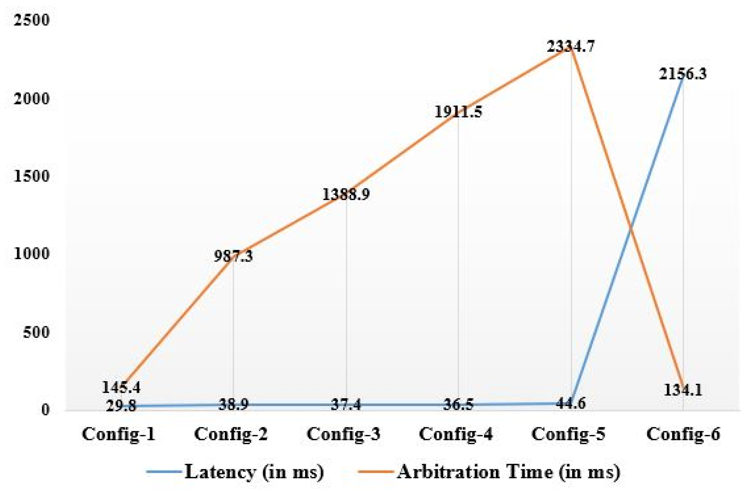
| Latency (in ms) | 29.8 | 38.9 | 37.4 | 36.5 | 44.6 | 2156.3 |
| Arbitration time (in ms) | 145.4 | 987.3 | 1388.9 | 1911.5 | 2334.7 | 134.1 |
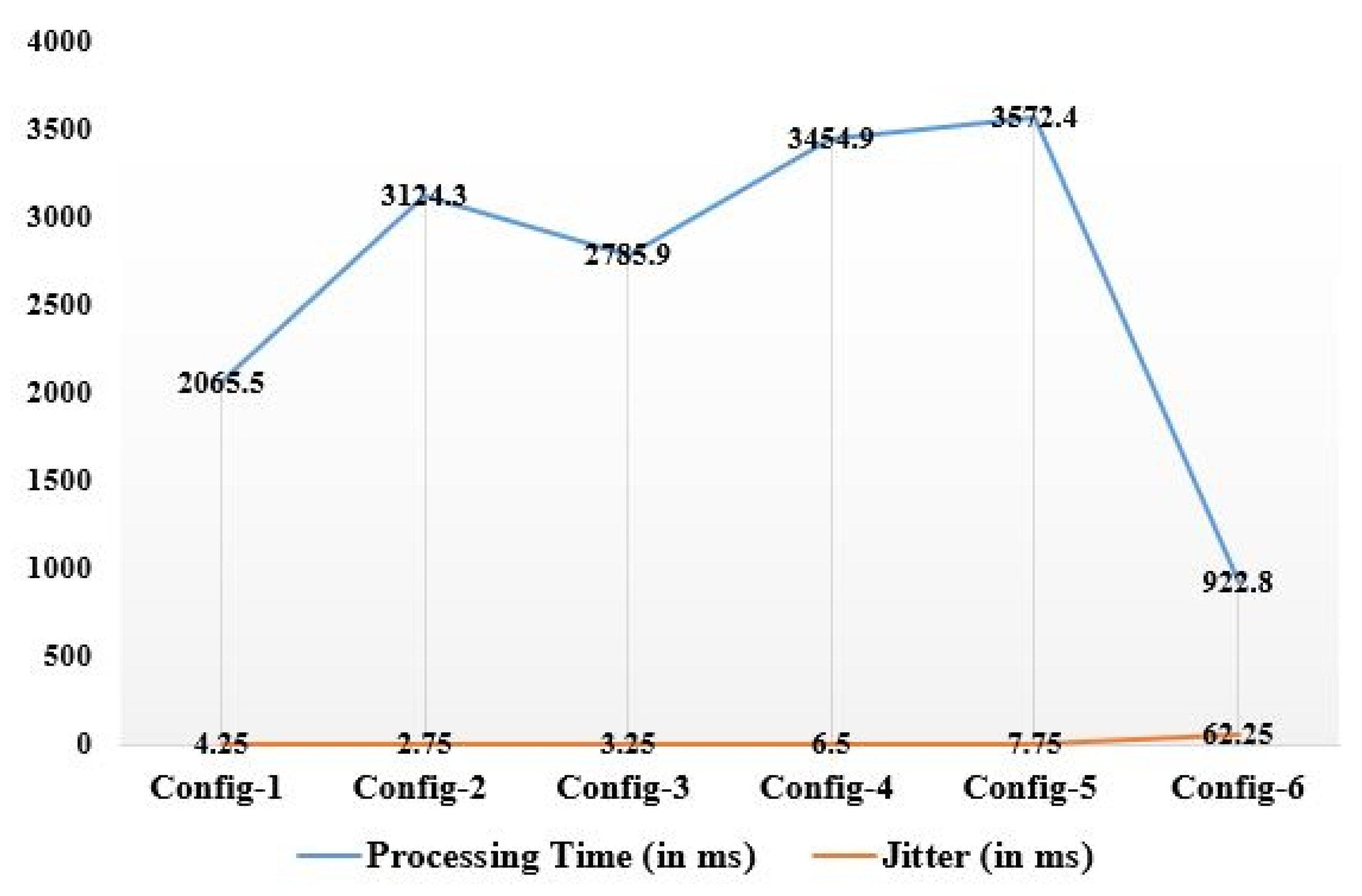
| Processing time (in ms) | 2065.5 | 3124.3 | 2785.9 | 3454.9 | 3572.4 | 922.8 |
| Jitter (in ms) | 4.25 | 2.75 | 3.25 | 6.50 | 7.75 | 62.25 |
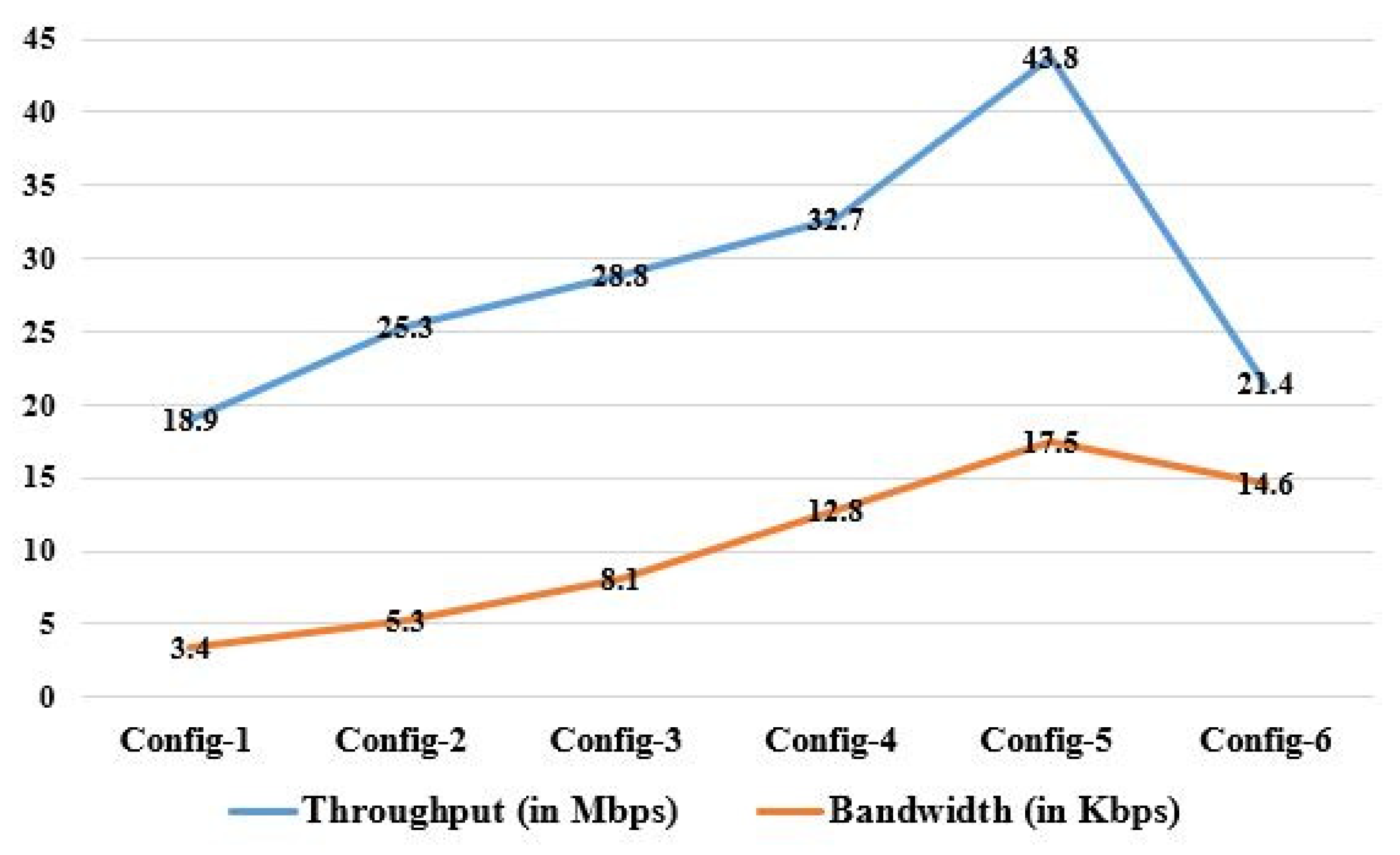
| Throughput (in Mbps) | 18.9 | 25.3 | 28.8 | 32.7 | 43.8 | 21.4 |
| Bandwidth (in Kbps) | 3.4 | 5.3 | 8.1 | 12.8 | 17.5 | 14.6 |
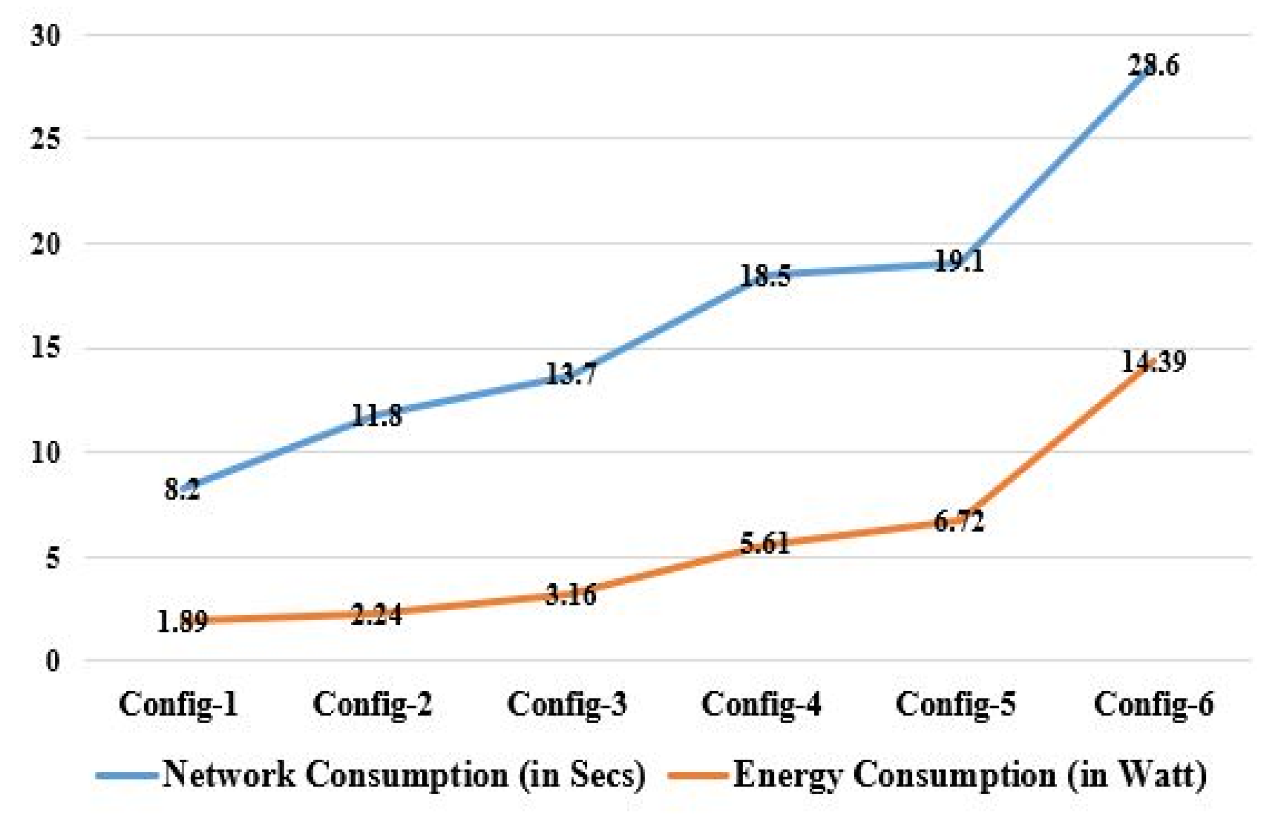
| Network consumption (in secs) | 8.2 | 11.8 | 13.7 | 18.5 | 19.1 | 28.6 |
| Energy consumption (in Watt) | 1.89 | 2.24 | 3.16 | 5.61 | 6.72 | 14.39 |
| Work | Methodologies | Dataset Employed | Findings (in %) | ||||
|---|---|---|---|---|---|---|---|
| ACC | PPV | TPR | TNR | F1S | |||
| [12] | CNN | Switzerland, LongBeach, Hungarian, and Cleveland HDDs | 89.74 | NA | 97.67 | 82.71 | NA |
| [13] | RNN | Datasets from PAMF and MIMIC–III | 63.87 | NA | NA | NA | NA |
| [14] | SDN and VANET | Real-time dataset | NA | NA | NA | NA | NA |
| [15] | KNN and GA | Hungarian HDD | 96.25 | NA | NA | NA | NA |
| [16] | NB, ANN, SVM, RF, and LR | Hungarian and Cleveland HDDs | 98.14 | 98.10 | 98.10 | NA | 98.10 |
| [17] | RF, LR, SVM, ELM, KNN, and Relief | Cleveland, Statlog, and Hungarian HDDs | NA | 92.59 | 92.15 | 93.21 | NA |
| [18] | ML and DL Methods | Cleveland and Hungarian HDDs | 98.50 | 98.20 | 96.40 | NA | 97.20 |
| [19] | NB, RF, KNN and SVM-Linear | Tele ECG | 69.90 | NA | NA | NA | 62.30 |
| [20] | CNN with BiLSTM or BiGRU | Mexico’s Medica Datasets | 98.00 | 99.00 | 96.00 | NA | 98.00 |
| [21] | RNN, LSTM, and SLAP | ECG dataset | 92.00 | NA | 92.00 | NA | 92.00 |
| [22] | ANN and EL Approaches | Cleveland HDD | 94.00 | NA | NA | NA | NA |
| [23] | LR, KNN, SVM, NB, RF, and HPO | Cleveland HDD | 90.78 | NA | NA | NA | NA |
| [24] | MLDS and ML Methods | Realistic dataset from Kaggle | 94.16 | 97.00 | 91.11 | 97.19 | NA |
| FRIEND [Proposed] | DNN, ML, and EL Approaches | IHDD | 94.27 | 97.59 | 96.09 | 75.44 | 96.83 |
| Work | ML | DL | EL | IoT | FC | Performance Parameters | ||||||||
|---|---|---|---|---|---|---|---|---|---|---|---|---|---|---|
| AT | LT | PT | TP | EC | BW | JT | NC | ACC | ||||||
| [12] | A | P | A | A | A | A | A | A | A | A | A | A | A | P |
| [13] | A | P | A | A | A | A | A | A | A | A | A | A | A | P |
| [14] | A | A | A | P | A | A | A | A | A | A | A | A | A | A |
| [15] | P | A | A | A | A | A | A | A | A | A | A | A | A | P |
| [16] | P | A | P | A | A | A | A | A | A | A | A | A | A | P |
| [17] | P | A | P | A | A | A | A | A | A | A | A | A | A | A |
| [18] | A | P | P | A | A | A | A | A | A | A | A | A | A | P |
| [19] | P | A | A | P | P | A | P | A | A | A | A | A | A | P |
| [20] | A | P | P | A | A | A | A | A | A | A | A | A | A | P |
| [21] | A | P | A | P | P | A | P | A | A | A | A | A | A | P |
| [22] | A | P | P | P | P | P | P | P | A | P | P | P | A | P |
| [23] | P | P | A | A | A | A | A | A | A | A | A | A | A | P |
| [24] | P | A | P | A | A | A | A | A | A | A | A | A | A | P |
| FRIEND [Proposed] | P | P | P | P | P | P | P | P | P | P | P | P | P | P |
Disclaimer/Publisher’s Note: The statements, opinions and data contained in all publications are solely those of the individual author(s) and contributor(s) and not of MDPI and/or the editor(s). MDPI and/or the editor(s) disclaim responsibility for any injury to people or property resulting from any ideas, methods, instructions or products referred to in the content. |
© 2023 by the authors. Licensee MDPI, Basel, Switzerland. This article is an open access article distributed under the terms and conditions of the Creative Commons Attribution (CC BY) license (https://creativecommons.org/licenses/by/4.0/).
Share and Cite
Pati, A.; Parhi, M.; Alnabhan, M.; Pattanayak, B.K.; Habboush, A.K.; Al Nawayseh, M.K. An IoT-Fog-Cloud Integrated Framework for Real-Time Remote Cardiovascular Disease Diagnosis. Informatics 2023, 10, 21. https://doi.org/10.3390/informatics10010021
Pati A, Parhi M, Alnabhan M, Pattanayak BK, Habboush AK, Al Nawayseh MK. An IoT-Fog-Cloud Integrated Framework for Real-Time Remote Cardiovascular Disease Diagnosis. Informatics. 2023; 10(1):21. https://doi.org/10.3390/informatics10010021
Chicago/Turabian StylePati, Abhilash, Manoranjan Parhi, Mohammad Alnabhan, Binod Kumar Pattanayak, Ahmad Khader Habboush, and Mohammad K. Al Nawayseh. 2023. "An IoT-Fog-Cloud Integrated Framework for Real-Time Remote Cardiovascular Disease Diagnosis" Informatics 10, no. 1: 21. https://doi.org/10.3390/informatics10010021