Article

Do We Need Stochastic Volatility and Generalised Autoregressive Conditional Heteroscedasticity? Comparing Squared End-Of-Day Returns on FTSE

by
David E. Allen
1,2,3,* and
Michael McAleer
2,4,5,6,7,8
1
School of Mathematics and Statistics, University of Sydney, Sydney 2006, Australia
2
Department of Finance, Asia University, Taichung 41354, Taiwan
3
School of Business and Law, Edith Cowan University, Joondalup 6027, Australia
4
Discipline of Business Analytics, University of Sydney Business School, Sydney, NSW 2006, Australia
5
Econometric Institute, Erasmus School of Economics, Erasmus University Rotterdam, 3062 Rotterdam, The Netherlands
6
Department of Economic Analysis and ICAE, Complutense University of Madrid, 28040 Madrid, Spain
7
Department of Mathematics and Statistics, University of Canterbury, Christchurch 8041, New Zealand
8
Institute of Advanced Sciences, Yokohama National University, Kanagawa 240-8501, Japan
*
Author to whom correspondence should be addressed.
Risks 2020, 8(1), 12; https://doi.org/10.3390/risks8010012
Submission received: 29 June 2019 / Revised: 12 December 2019 / Accepted: 13 January 2020 / Published: 1 February 2020
(This article belongs to the Special Issue Measuring and Modelling Financial Risk and Derivatives)

Abstract

:
The paper examines the relative performance of Stochastic Volatility (SV) and Generalised Autoregressive Conditional Heteroscedasticity (GARCH) (1,1) models fitted to ten years of daily data for FTSE. As a benchmark, we used the realized volatility (RV) of FTSE sampled at 5 min intervals taken from the Oxford Man Realised Library. Both models demonstrated comparable performance and were correlated to a similar extent with RV estimates when measured by ordinary least squares (OLS). However, a crude variant of Corsi’s (2009) Heterogeneous Autoregressive (HAR) model, applied to squared demeaned daily returns on FTSE, appeared to predict the daily RV of FTSE better than either of the two models. Quantile regressions suggest that all three methods capture tail behaviour similarly and adequately. This leads to the question of whether we need either of the two standard volatility models if the simple expedient of using lagged squared demeaned daily returns provides a better RV predictor, at least in the context of the sample.

1. Introduction

The paper explores the performance of Stochastic Volatility (SV) and Generalised Autoregressive Conditional Heteroscedasticity (GARCH) (1,1) models as estimators of the volatility of the FTSE Index. The volatilities estimated by these models are compared with realised volatility estimates for FTSE, obtained from the Oxford Man Realised Library and sampled at 5 min intervals, as described in Heber et al. (2009). Their volatility forecasts were further compared with those derived from a simple historical volatility model.
We used the stochvol R package, which uses Markov chain Monte Carlo (MCMC) samplers, to conduct inference by obtaining draws from the posterior distribution of parameters and latent variables, which could then be used for predicting future volatilities. This is done within the context of a fully Bayesian implementation of heteroscedasticity modelling within the framework of stochastic volatility. For more information, see the discussion of the method by Kastner and Frühwirth-Schnatter (2014), and of the stochvol package by Kastner (2016).
Taylor (1982) suggested probabilistically modelling volatility, in effect through a state-space model where the logarithm of the squared volatilities, the latent states, follows an autoregressive process of order one. Over time, this specification became known as the SV model. A series of early papers by Jacquier et al. (1994), Ghysels et al. (1996), and Kim et al. (1998) provided evidence in support of the application of stochastic-volatility models, but their practical use has been infrequent. The reasons for this were considered by Bos (2012), who suggested that the empirical application of SV models was limited by two major factors: the variety (and potential incompatibility) of estimation methods for SV models and the lack of standard software packages for implementing these methods. The situation for multivariate SV is even more problematic.
Taylor (1994) provides a review of both stochastic volatility and the ARCH/GARCH literature. More recent reviews of the use of inference in the context of this literature were provided by McAleer (2005), and a review of multivariate stochastic-volatility models was provided by Asai et al. (2006). Granger and Poon (2003, p. 485), in their review of volatility-forecasting methods, noted the difficulties in the application of the SV model: “the SV model has no closed form, and hence cannot be estimated directly by maximum likelihood”. They also noted that the quasimaximum-likelihood method may also be inefficient if the volatility proxies are non-Gaussian. The advantage of the stochvol R package is that it incorporates an efficient MCMC estimation scheme for SV models, as discussed by Kastner and Frühwirth-Schnatter (2014). This facilitated analysis in this paper, which features a direct comparison of the volatility predictions of a SV model, a GARCH (1,1) model, and a simple application of a historical-volatility-based estimation method, as applied to the FTSE index.
The paper is divided into four sections: Section 2 reviews the literature and employed econometric method. Section 3 presents the results, and Section 4 concludes the paper.

2. Previous Work and Econometric Models

2.1. Stochastic Volatility

There have been numerous empirical studies of changes in volatility in various stock, currency, and commodity markets. Findings in volatility research have implications for option pricing, volatility estimation, and the degree to which volatility shocks persist. These research questions have been approached by means of different models and methodologies.
Taylor (1982) suggested a novel SV approach, and Taylor (1994) implemented the SV model as follows: if P t denotes the prices of an asset at time t , and assuming no dividend payments, returns on the asset can be defined, in the context of discrete time periods, as:
X t = l n [ P t / P t 1 ] .
Volatility is customarily indicated by σ , and prices are described by a stochastic differential equation:
d ( l n P ) = μ d t + σ d W ,
with W being a standard Weiner process. If μ and σ are constants, X t has normal distribution, and
X t = μ + σ U t ,
with U t being independent and identically distributed ( i . i . d ) .
Equation (3) can be generalised by replacing σ with positive random variable σ t to give:
X t = μ + σ t U t ,
where U t N ( 0 , 1 ) .
In circumstances where returns process { X t } can be presented by Equation (4), Taylor (1994) called σ t the stochastic volatility for period t. His definition assumed that ( X t μ ) / σ t follows normal distribution.
Stochastic process { σ t } generates realised volatilities { σ t } that, in general, are not observable. For any realisation, σ t
X t σ t = σ t N ( μ , σ t 2 ) .
The mixture of these conditional normal distributions defines the unconditional distribution of X t , which has excess kurtosis whenever σ t has positive variance and is independent of U t .
In the empirical section that follows, we used the RV of the FTSE sampled at 5 min intervals, provided by Oxford Man, as a proxy for true realised volatility. We then compared the estimates of volatility obtained from the SV and GARCH (1,1) models by using the RV estimates as a benchmark.
Taylor (1994, p. 3) suggested using “capital letters to represent random variables and lowercase letters to represent outcomes”, and we follow that convention. Given the observed returns of I t 1 = { x 1 , x 2 , . x t 1 } , the conditional variance for period t is:
h t = v a r ( X t I t 1 ) .
Taylor (1994) notes that, in general, random variable H t , which generates observed conditional variance h t , is not, in general, equal to σ t 2 . A convenient way to use economic theory to motivate changes in volatility is to assume that returns are generated by a number of intraperiod price revisions, as in the manner of Clark (1973) and Tauchen and Pitts (1983), to mention two of many studies.
It is assumed that there are N t price revisions during trading day t, each caused by unpredictable information. Let event i on day t change the logarithmic price by ω i t , with
X t = μ + i = 1 N t ω i t .
If we assume that ω i t i . i . d . and is independent of random variable N t , with ω i t N ( 0 , σ ω 2 ) , then
σ t 2 = σ ω 2 N t a n d H t = σ ω 2 E [ N t I t 1 ] .
The above model suggests that squared volatility is proportional to the amount of price information.
The lack of standard software to estimate such a model is addressed by Kastner and Frühwirth-Schnatter (2014), who proposed an efficient MCMC estimation scheme that is implemented in the R stochvol package (Kastner (2016)). Kastner (2016, p. 2) proceeded by “letting y = ( y 1 , y 2 , . y n ) | be a vector of returns, with mean zero. An intrinsic feature of the SV model is that each observation y t is assumed to have its ’own’ contemporaneous variance, e h t , which relaxes the usual assumption of homoscedasticity”. It was assumed that the logarithm of this variance follows an autoregressive process of order one. This assumption is fundamentally different to GARCH models, where time-varying conditional volatility is assumed to follow deterministic instead of stochastic evolution.
The centered parameterization of the SV model can be given as:
y t h t N ( 0 , e x p h t ) ,
h t h t 1 , μ , ϕ , σ n N ( μ , + ϕ ( h t 1 μ ) , σ n 2 ) ,
h 0 μ , ϕ , σ n N ( μ , σ n 2 / ( 1 ϕ 2 ) ,
where N ( μ , σ n 2 ) , denotes normal distribution with mean μ and variance σ n 2 . θ = ( μ , ϕ , σ n ) | is the vector of parameters that consists of the level of log variance μ , the persistence of log variance, ϕ , and volatility of log variance σ n . Process h = ( h 0 , h 1 , , h n ) | , which features in Equations (10) and (11), is the unobserved or latent time-varying volatility process.
Kastner (2016, p. 4) remarked that: “A novel and crucial feature of the algorithm implemented in stochvol is the usage of a variant of the “ancillarity–sufficiency interweaving strategy” (ASIS) which has been brought forward in the general context of state-space models by Yu and Meng (2011). ASIS exploits the fact that, for certain parameter constellations, sampling efficiency improves substantially when considering a non-centered version of a state-space model”.
Another key feature of the algorithm used in stochvol is the joint sampling of all instantaneous volatilities “all without a loop” (AWOL), a technique with links to Rue (2001) that is discussed in McCausland et al. (2011). The combination of these features enables the stochvol R package to efficiently estimate SV models even when large datasets are involved.

2.2. ARCH and GARCH

Engle (1982) developed the Autoregressive Conditional Heteroscedasticity (ARCH) model that incorporates all past error terms. It was generalised to GARCH by Bollerslev (1986) to include lagged term conditional volatility. In other words, GARCH predicts that the best indicator of future variance is a weighted average of long-run variance, the predicted variance for the current period, and any new information in this period, as captured by the squared residuals.
The framework was developed as follows: consider a time series y t = E t 1 ( y t ) + ε t , where E t 1 ( y t ) is the conditional expectation of y t at time t 1 , and ε t is the error term. The basic GARCH model has the following specification:
ε t = h t η t , η t N ( 0 , 1 )
h t = ω + j = 1 p α j ε t j 2 + j = 1 q β j h t j
in which ω > 0 , α j 0 and β j 0 (usually a positive fraction), to ensure a positive conditional variance, h t 0 (see Tsay (1987)). The ARCH effect is captured by parameter α j , which represents the short-run persistence of shocks to returns, β j captures the GARCH effect that contributes to long-run persistence, and α j + β j measures the persistence of the impact of shocks to returns to long-run persistence. A GARCH (1,1) process is weakly stationary if α j + β j 1 (see the discussion in Allen et al. (2013)).
We contrasted the estimates of volatility from the SV model with those from a GARCH (1,1) model, and assessed which better explained the behaviour of the RV of FTSE sampled at 5 min intervals.

2.3. Realised Volatility

We used the 5 min RV estimates from Oxford Man for FTSE as the RV benchmark (see: https://realized.oxford-man.ox.ac.uk/data). Their database contains “daily (close-to-close) financial returns, and a corresponding sequence of daily realised measures r m 1 , r m 2 , . . , r m T . Realised measures are theoretically sound, high-frequency, nonparametric-based estimators of the variation of the price path of an asset during the times in which the asset trades frequently on an exchange. Realised measures ignore the overnight variation of prices, and sometimes the variation in the first few minutes of the trading day, when recorded prices may contain large errors”. The metrics were developed by Andersen et al. (2001), Andersen et al. (2003), and Barndorff-Nielsen and Shephard (2002). Shephard and Sheppard (2010) provide an account of RV measures used in the Oxford Man Realised Library.
The simplest realised metric is realised variance (RV):
R V t = x j , t 2 ,
where x j , t = X t j , t X t j 1 , t . The t j , t are the times of trades or quotes on the t-th day. The theoretical justification of this measure is that, if prices are observed without noise, then, as m i n j t j , t t j 1 , t 0 , it consistently estimates the quadratic variation of the price process on the t-th day. If sampling is reduced to very small time intervals, market-microstructure noise may become a contaminant. In order to avoid this issue, we used RV estimates from Oxford Man, sampled at 5 min intervals, hereafter R V 5 .

2.4. Historical-Volatility Model

Poon and Granger (2005) discussed various practical issues encountered in attempts to forecast volatility. They suggested that the HISVOL model has the following form:
σ ^ t = ϕ 1 σ t 1 + ϕ 2 σ t 2 + . . + ϕ τ σ t τ ,
where σ ^ t is the expected standard deviation at time t, ϕ is the weight parameter, and σ is the historical standard deviation for periods indicated by the subscripts. Poon and Granger (2005) suggested that this group of models include random walk, historical averages, autoregressive (fractionally integrated) moving average, and various forms of exponential smoothing that depend on weight parameter ϕ .
We used a simple form of this model in which the estimate of σ is the previous day’s demeaned squared return. Poon and Granger (2005) noted that, in a review of 66 previous studies, implied standard deviations appeared to perform best, followed by historical volatility and GARCH, which have roughly equal performance. They also noted that, at the time of writing, there were insufficient studies of SV models to come to any conclusions about this class of models. This is a motivation for the current study that assesses the performance of all three classes of models.
Barndorff-Nielsen and Shephard (2003) pointed out that taking the sums of squares of increments of log prices has a long tradition in the financial economics literature. Early examples are Poterba and Summers (1986), Schwert (1989), Taylor and Xu (1997), Christensen and Prabhala (1998), Dacorogna et al. (1998), and Andersen et al. (2001). Shephard and Sheppard (2010, p. 200, footnote 4) noted that: “Of course, the most basic realised measure is the squared daily return”. We utilised this approach as the basis of our historical-volatility model.

2.5. Heterogeneous Autoregressive Model (HAR)

Corsi (2009, p. 174) suggested “an additive cascade model of volatility components defined over different time periods. The volatility cascade leads to a simple AR-type model in the realized volatility with the feature of considering different volatility components realized over different time horizons and which he termed as a Heterogeneous Autoregressive model of Realized Volatility.” Corsi (2009) suggested that the model successfully achieves the purpose of reproducing the main empirical features of financial returns (long memory, fat tails, and self-similarity) in a parsimonious way. He wrote his model as:
σ t + 1 d ( d ) = c + β ( d ) R V t ( d ) + β ( w ) R V t ( w ) + β ( m ) R V t ( m ) + ω ˜ t + 1 d ( d ) ,
where σ ( d ) is daily integrated volatility, and R V t ( d ) , R V t ( w ) and R V t ( m ) are the daily, weekly, and monthly (ex post) observed realized volatilities, respectively.
We appealed to Corsi (2009) to inspire our HISVOL model, which uses lags of historical RV estimates, but we used lags of squared demeaned daily returns.

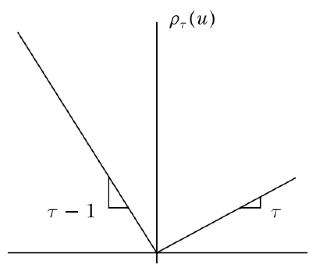
2.6. Quantile Regression

We used the RV5 estimates as a benchmark to assess how the SV and GARCH(1,1) models performed. We were interested in behaviour in the extreme tails as well as in the centre of distribution. We therefore used quantile regression to assess behaviour in the tails.
Koenker and Hallock (2001, p. 145) provided an introduction to quantile regression, and noted that “quantiles seem inseparably linked to the operations of ordering and sorting the sample observations that are usually used to define them”. They added: “The symmetry of the piecewise linear absolute value function implies that the minimization of the sum of absolute residuals must equate the number of positive and negative residuals, thus assuring that there are the same number of observations above and below the median”.
They asked: What about the other quantiles? As the symmetry of the absolute value yields the median, it follows that minimising the sum of asymmetrically weighted absolute residuals by simply giving differing weights to positive and negative residuals provides the other quantiles. The solution to
M i n ξ R ρ τ ( y i ξ ) ,
where function ρ τ ( · ) is the titled absolute value function, shown in Figure 1, gives the τ th sample quantile function.
An estimate of the conditional median function can be obtained by replacing scalar ξ in Equation (10) by parametric function ξ ( x i , β ) , and setting τ to 1 / 2 . Estimates of the other conditional quantile functions can be obtained by replacing absolute values by ρ τ ( · ) , and solving Expression (11) by linear programming:
m i n β R p ρ τ ( y i ξ ( x i , β ) .
We applied quantile regression to investigate the relationship between RV5 estimates on the FTSE Index and risk values predicted by the SV and GARCH(1,1) models.

3. Analysis Results

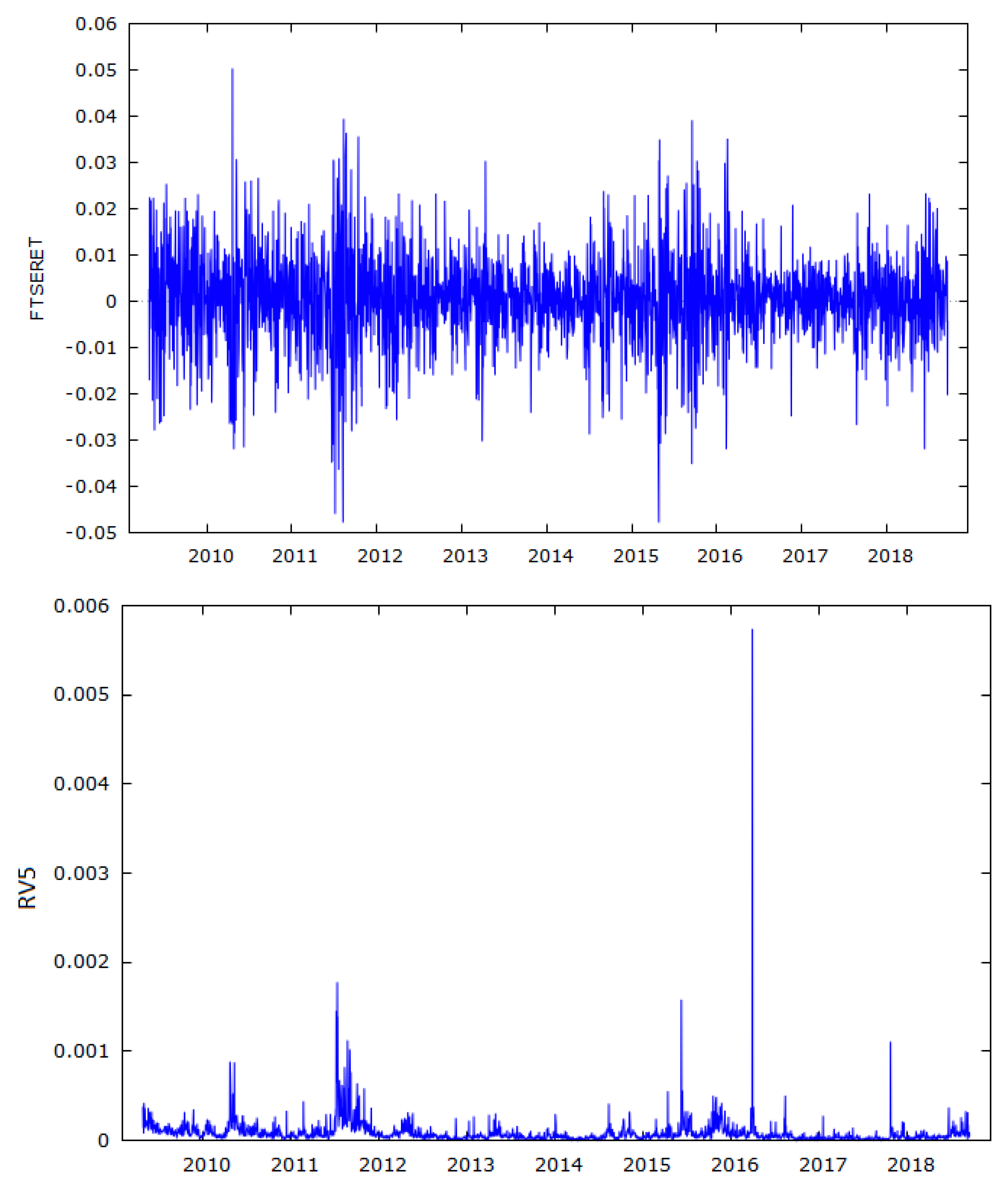
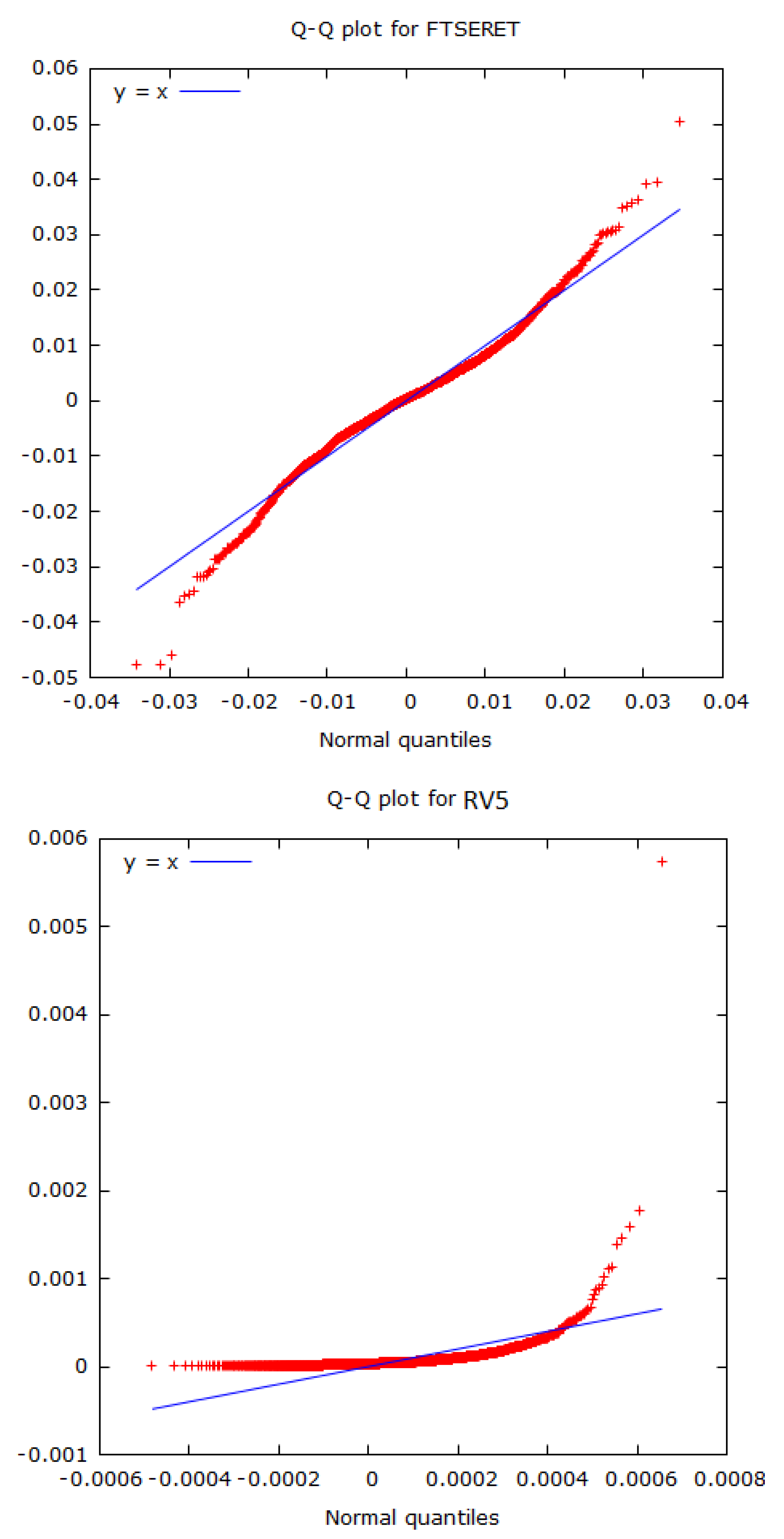
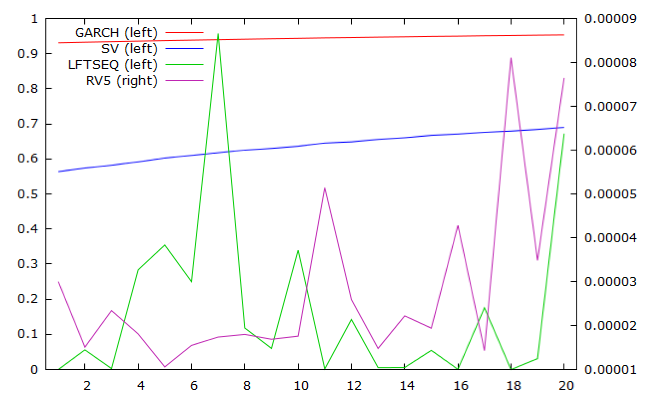
3.1. Preliminary Analysis

The sample dataset consisted of approximately 10 years of daily data of adjusted continuously compounded returns for FTSE, from 24 April 2009 through to 16 April 2019, sourced from Yahoo Finance via the R quantmod library. However, we retained the last 20 observations from the series for forecast purposes, leaving a total of 2454 observations. A matching set of daily RV5 estimates for FTSE was obtained from the Oxford Man Realised Library. Summary statistics for the two series is provided in Table 1 and plots of the two series in Figure 2.
FTSE has a mean daily return of 0.02% and a standard deviation of 0.97%. It has positive excess kurtosis and does not conform to Gaussian distribution, as can be seen from the QQ plot in Figure 3. RV5 has a mean of 8.6261 × 10 5 and a standard deviation of 0.00016097. However, it is measured as a variance, and if we take the square root of its value and multiply it by 100, it is on a common scale with the FTSE returns. We undertook this transformation in some of the comparison plots in subsequent figures. It has very high skewness and kurtosis, which is also evident in the QQ plots in Figure 3.

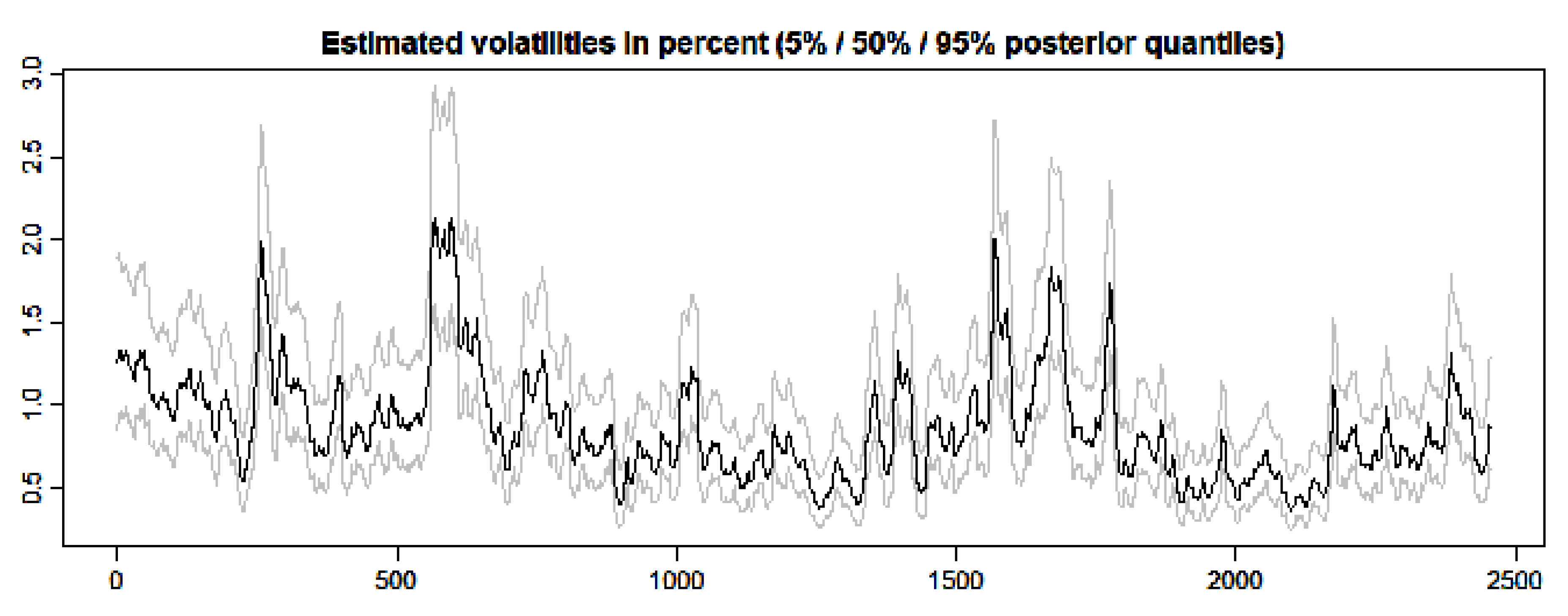
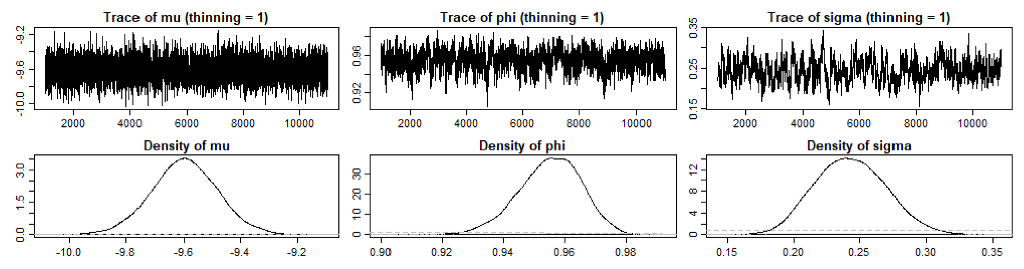
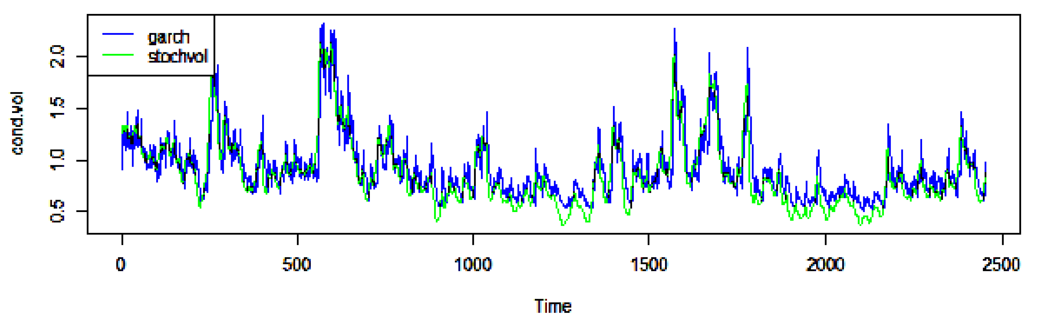
3.2. SV and GARCH Estimates

We used R library stochvol to fit a stochastic-volatility model to the FTSE return series, and used Gaussian distributions to fit the SV model. Some of the initial parameters for SV model estimation are shown in Table 2. The SV model applied to FTSE produced the volatility estimates shown in Figure 4, while Figure 5 displays a kernel-density estimate for parameters contained in θ, producing posterior-density estimates. Figure 4 plots the estimated volatilities produced by the SV model at the 5%, 50%, and 95% posterior quantiles.
We also estimated GARCH (1,1) to obtain conditional volatilities. Coefficients are shown in Figure 3. The diagnostic tests suggested that there were no ARCH effects in the residuals, but rejected the null hypothesis that residuals conform to normal distribution. Plots of the volatilities obtained from both the SV and GARCH (1,1) estimates are shown in Figure 6.
Table 3 confirms that SV estimates were slightly lower than GARCH(1,1) estimates. Mean SV estimate was 0.87152, while mean GARCH(1,1) volatility estimate was 0.92405. This difference is significant, as revealed by a nonparametric sign test, the results of which are available from the authors on request. The interquartile range for the SV model is 0.38324, while that for GARCH(1,1) was slightly smaller with a value of 0.32905. This is reflected in the standard deviations of the estimates, with a value of 0.32600 for the SV model, and 0.30490 for the GARCH(1,1). (Details of the GARCH model fitted are provided in Table 4).
The third panel in Table 3 provides summary statistics for SQRV5L which is the square root of realised volatility series RV5, scaled by 100, to transform it into the same dimension as the two conditional-volatility series. Mean value was markedly greater at 0.81989, standard deviation was also larger at 0.43644, while the interquartile range was 0.44676. Excess kurtosis was much greater, with a value of 29.966, given that the SV and GARCH(1,1) models had excess kurtosis of 1.9519 and 3.3669, respectively.
These statistics suggest that the modelfree estimate of volatility, provided by RV5, was more volatile and had larger spikes than the conditional volatilities produced by the two models.
We also estimated some regressions to explore the linear correlations between the estimates of the two volatility models and our base RV5 volatility estimates. In order to keep the values in the same dimension, we used the SQRV5L values. Results are shown in Table 5. If we used the RV5 values in the form of SQRV5L as the benchmark dependent variable, then conditional volatilities from the SV model had an adjusted R-square of 0.193842, and a highly significant slope coefficient with a value of 0.589930 and t-statistic of 24.31. The GARCH(1,1) model performs slightly better, with an adjusted R-squared of 0.202789 and a slope coefficient of 0.645116, with a t statistic of 25. The Durbin–Watson statistic for both models was around 1, suggesting that there iswasa borderline problem of serial correlation in the residuals.
As a further cross-check of the effectiveness of the two models, we used a further crude estimate of volatility with the demeaned squared daily returns on FTSE in the context of a HISVOL model, which was motivated by Corsi’s (2009) Heterogeneous Autoregressive model of Realized Volatility (HAR-RV).
In the third panel, we used the attribute that the squared demeaned returns on the FTSE are highly persistent, or have long memory, and regressed the square root of RV5 scaled by 100 on 28 lags of the squared demeaned FTSE return, also scaled by 100.
This crude model produced better results than those using SV and GARCH(1,1) conditional volatilities as explanatory variables. The adjusted R-squared value was 0.302940, and coefficients on lags of 3, 4, 5, 9, 11, 12, 13, 15, 17, 19, 21, 23, 24, 25, 27, and 28 of LSQDMFTSE were highly significant. The F statistic was highly significant, and the Durbin Watson statistic was slightly improved at 1.1399.
Plots of the volatility series are shown in Figure 7. In the upper panel of Figure 7, SQRV5 is plotted on a different scale to the two conditional volatilities so they were not superimposed on each other. In the lower panel, correspondence between RV5 and the crude measure of demeaned squared daily returns on the FTSE is evident.
Figure 8 provides a plot of actual versus fitted values when SQRV5L was regressed on 28 lags of LSQDMFTSE. Again, the effectiveness of the model is apparent. Figure 9 shows the predicted values of the conditional volatilities from the SV and GARCH, indexed on the L.H.S. of Figure 9, and the lagged values DMSQFTSERET plus the actual RV5 value for the day. The latter two series are indexed on the R.H.S. of Figure 9. If we rescaled the values of the latter two variables, it is apparent that there was closer proximity between them than from the predictions of SV and GARCH, even in the case of the first observation in the graph.
A potential issue was whether the relationship was significant in the quantiles, as this is an issue for risk measurement. In Table 6, we report the results of estimating quantile regressions for the same series.

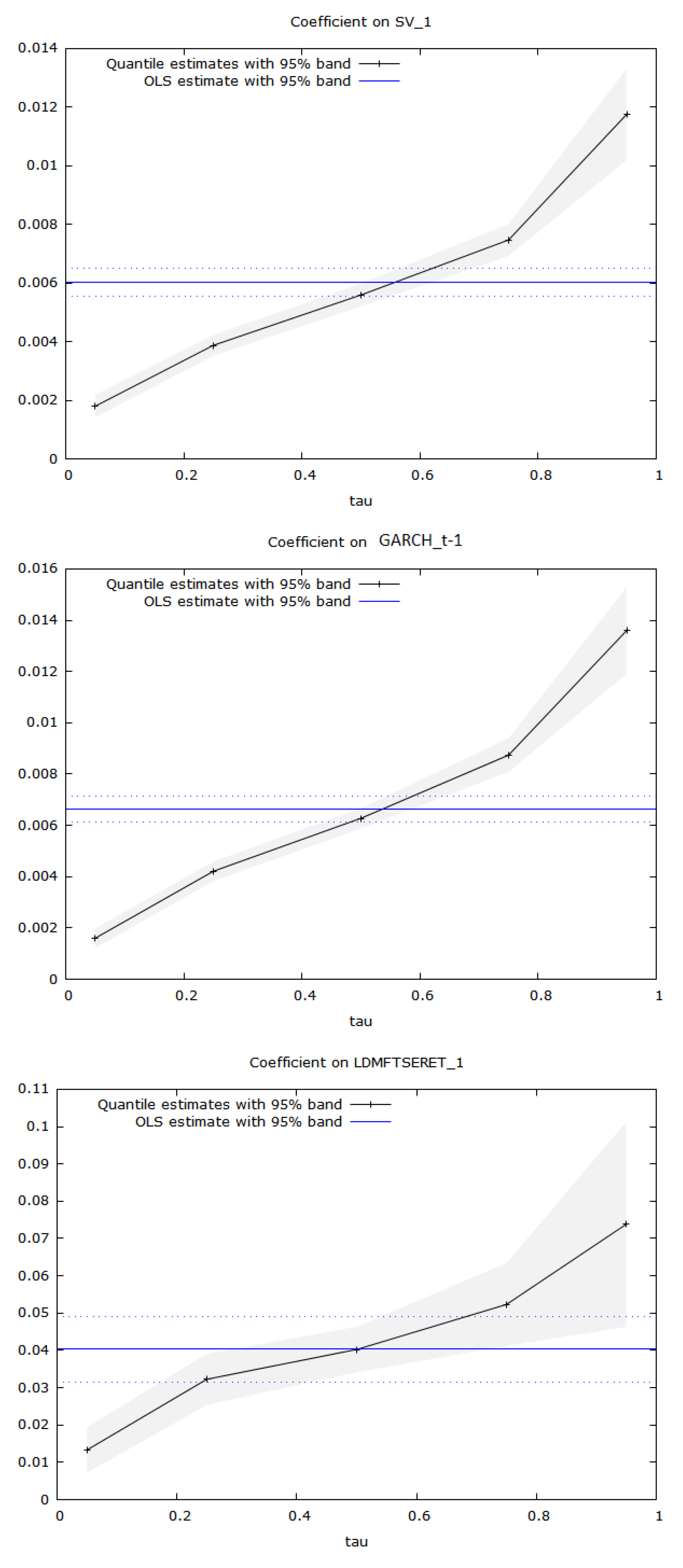
3.3. Quantile-Regression Results

The results of SQRV5L quantile regression on the lags of the three explanatory series are shown in Table 6. All three quantile regressions used SQRV5L as the dependent variable, adopting the modelfree RV5 estimation as the benchmark. We adopted tau values of 0.05, 0.25, 0.50, 0.75, and 0.95. Our concern was whether there was evidence of significant relationships across quantiles. All t statistics were significant at the 1% level across all quantiles. In the case of the third panel in Table 6, we only used one lag of the squared demeaned FTSE return, rather than the full model, to avoid excessive numbers of entries in the Tables. Even so, coefficients on all quantiles were significant at the 1% level.
Plots of these relationships are provided in Figure 10. The horizontal blue lines in the panels in Figure 10 depict least-squares regression coefficients, and the dotted lines above and below them depict the error bands. The black line links the coefficients estimated by quantile regression, and the grey area around the line shows the error bands. An interesting feature of the quantile-regression coefficients was that all three black lines in Figure 10 have positive slopes. This is consistent with the existence of more elastic responses to estimates in higher quantiles of RV5 volatility, in all three cases of SV, GARCH(1,1), and squared demeaned returns on FTSE, as predictors of volatility. Results suggested that none of these models was fully successful in capturing volatility peaks in RV5 in the higher quantiles.

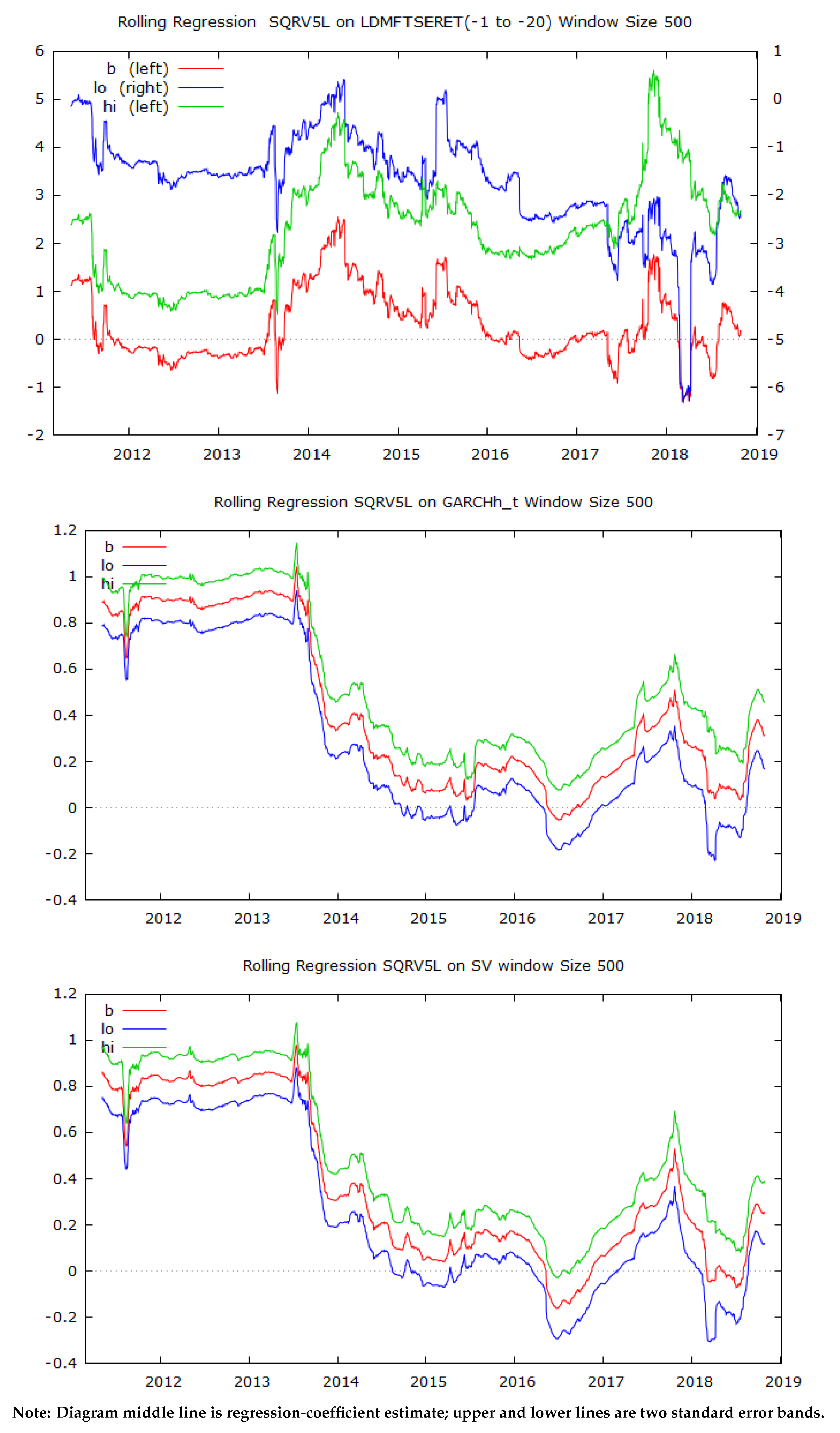
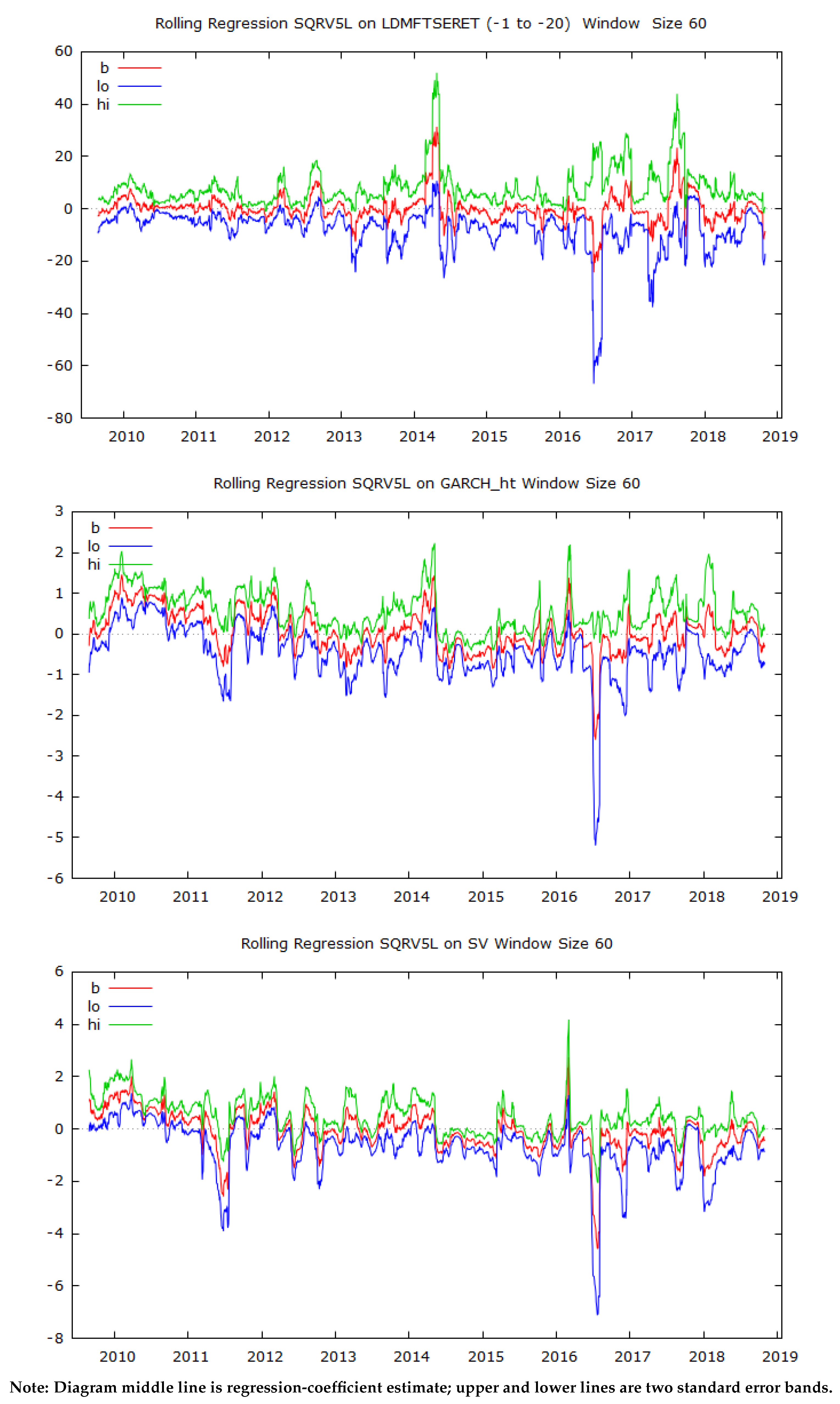
3.4. Rolling-Regression Analysis

As a further check, we ran some rolling regressions of our three daily volatility estimates from the three models of STOCHVOL, GARCH (1,1) and HISVOL as the explanatory variable for the realised RV5 estimates, using window sizes of 60 and 500 days.These window sizes were chosen to approximate three months and two years of daily returns. Graphs of the coefficient estimates from these three regressions, plus error bands of plus and minus two standard deviations, are shown in the Appendix A.
These plots suggest that, when we used the longer windows of 500 observations, the three models were significant around 50% of the time, in that the error bands did not span zero. None of the three models performed well in the 60 observation windows, and spanned zero for the majority of the considered period. The HISVOL model performed poorly in these short windows.

4. Conclusions

The paper featured an examination of the effectiveness of SV and GARCH(1,1) models as explainers of modelfree estimates of FTSE volatility using RV samples at 5 min intervals as a benchmark, as provided by Oxford Man Institute’s Realised Library. In order to provide further contrast, we also used lags of squared demeaned daily returns on FTSE to provide a simple alternative estimate of daily volatility. The effectiveness of these three methods was explored via the application of ordinary-least-squares (OLS) regression and quantile-regression analysis. Poon and Granger (2005) provided motivation in their analysis of 66 studies of this topic in which they noted that, at that time, there were an insufficient number of SV studies to provide a comparison between the GARCH and HISVOL models. Our intention was to address this sparsity in the literature.
We used vanilla estimates of SV and GARCH(1,1) by adopting Gaussian distributions. If measured by adjusted R-squared values, GARCH(1,1) appeared to produce slightly better OLS predictions than the SV model. However, both performed relatively poorly as compared with the simple expedient of using squared demeaned daily returns on FTSE to predict RV5 volatility. Our results support Poon and Granger (2005), in that neither the GARCH nor the SV model outperformed a simple form of a HISVOL model on this FTSE sample when RV samples at 5 min intervals were used as a benchmark. However, all three models performed poorly within short 60 observation windows in the rolling regressions. This suggests that the HISVOL model performs better over a longer observation window and is likely to be of more practical applications over longer holding periods.

Author Contributions

Conceptualization, D.E.A. and M.M.A.; methodology, D.E.A.; software, D.E.A.; validation, D.E.A., and M.M.A.; formal analysis, D.E.A.; investigation, M.M.A.; resources, M.M.A.; data curation, D.E.A.; writing–original draft preparation, D.E.A.; writing–review and editing, M.M.A.; project administration, M.M.A.; funding acquisition, M.M.A. All authors have read and agreed to the published version of the manuscript.

Funding

This research received no external funding.

Conflicts of Interest

The authors declare no conflict of interest.

Appendix A

Figure A1. Rolling-regression—window size 500.
Risks 08 00012 g0a1
Figure A2. Rolling-regression—window size 60.
Risks 08 00012 g0a2

References

  1. Allen, David E., Ron Amram, and Michael McAleer. 2013. Volatility spillovers from the Chinese stock market to economic neighbours. Mathematics and Computers in Simulation 94: 238–57. [Google Scholar] [CrossRef] [Green Version]
  2. Andersen, Torben G., Tim Bollerslev, Francis X. Diebold, and Heiko Ebens. 2001. The distribution of realized stock return volatility. Journal of Financial Economics 61: 43–76. [Google Scholar] [CrossRef]
  3. Andersen, Torben G., Tim Bollerslev, Francis X. Diebold, and Paul Labys. 2003. Modeling and forecasting realized volatility. Econometrica 71: 529–626. [Google Scholar] [CrossRef] [Green Version]
  4. Asai, Manabu, Michael McAleer, and Jun Yu. 2006. Multivariate stochastic volatility: A review. Econometric Reviews 25: 145–75. [Google Scholar] [CrossRef]
  5. Barndorff-Nielsen, Ole E., and Neil Shephard. 2002. Econometric analysis of realised volatility and its use in estimating stochastic volatility models. Journal of the Royal Statistical Society, Series B 63: 253–80. [Google Scholar] [CrossRef]
  6. Barndorff-Nielsen, Ole E., and Neil Shephard. 2003. Realized power variation and stochastic volatility models. Bernoulli 9: 243–65. [Google Scholar] [CrossRef]
  7. Bollerslev, Tim. 1986. Generalized autoregressive conditional heteroskedasticity. Journal of Econometrics 31: 307–27. [Google Scholar] [CrossRef] [Green Version]
  8. Bos, Charles S. 2012. Relating stochastic volatility estimation methods. In Handbook of Volatility Models and Their Applications. Edited by Luc Bauwens, Christian Hafner and Sebastien Laurent. New York: John Wiley & Sons, pp. 147–74. [Google Scholar]
  9. Christensen, Bent J., and Nagpurnanand R. Prabhala. 1998. The relation between implied and realized volatility. Journal of Financial Economics 37: 125–50. [Google Scholar] [CrossRef]
  10. Clark, Peter K. 1973. A subordinated stochastic process model with finite variance for speculative prices. Econometrica 41: 135–55. [Google Scholar] [CrossRef]
  11. Corsi, Fulvio. 2009. A simple approximate long-memory model of realized volatility. Journal of Financial Econometrics 7: 174–96. [Google Scholar] [CrossRef]
  12. Dacorogna, Michel M., Ulrich A. Müller, Olivier V. Pictet, and Richard B. Olsen. 1998. Modelling short term volatility with GARCH and HARCH. Edited by Christian Dunis and Bin Zhou. Nonlinear Modelling of High Frequency Financial Time Series; Chichester: Wiley. [Google Scholar]
  13. Engle, Robert F. 1982. Autoregressive conditional heteroskedasticity with estimates of the variance of United Kingdom inflation. Econometrica 50: 987–1007. [Google Scholar] [CrossRef]
  14. Ghysels, Eric, Andrew C. Harvey, and Eric Renault. 1996. Stochastic volatility. In Statistical Methods in Finance, Volume 14, Handbook of Statistics. Edited by Gangadharrao Soundalyarao Maddala and Calyampudi Radhakrishna Rao. Amsterdam: Elsevier, pp. 119–91. [Google Scholar]
  15. Heber, Gerd, Asger Lunde, Neil Shephard, and Kevin Sheppard. 2009. Oxford-Man Institute’s Realized Library. Oxford: Oxford-Man Institute, University of Oxford. [Google Scholar]
  16. Jacquier, Eric, Nicholas G. Polson, and Peter E. Rossi. 1994. Bayesian analysis of stochastic volatility models. Journal of Business & Economic Statistics 12: 371–89. [Google Scholar]
  17. Kastner, Gregor, and Sylvia Frühwirth-Schnatter. 2014. Ancillarity-sufficiency interweaving strategy (ASIS) for boosting MCMC estimation of stochastic volatility models. Computational Statistics and Data Analysis 76: 408–23. [Google Scholar] [CrossRef] [Green Version]
  18. Kastner, Gregor. 2016. Dealing with stochastic volatility in time series using the R package stochvol. Journal of Statistical Software 69: 1–30. [Google Scholar] [CrossRef] [Green Version]
  19. Kim, Sangjoon, Neil Shephard, and Siddhartha Chib. 1998. Stochastic volatility: Likelihood inference and comparison with ARCH models. Review of Economic Studies 65: 361–93. [Google Scholar] [CrossRef]
  20. Koenker, Roger, and Kevin F. Hallock. 2001. Quantile regression. Journal of Economic Perspectives 15: 143–56. [Google Scholar] [CrossRef]
  21. McAleer, Michael. 2005. Automated inference and learning in modeling financial volatility. Econometric Theory 21: T232–61. [Google Scholar] [CrossRef] [Green Version]
  22. McCausland, William J., Shirley Miller, and Denis Pelletier. 2011. Simulation smoothing for state-space models: A computational efficiency analysis. Computational Statistics and Data Analysis 55: 199–212. [Google Scholar] [CrossRef]
  23. Poon, Ser-Huang, and Clive W. J. Granger. 2003. Forecasting volatility in financial markets: A review. Journal of Economic Literature 41: 478–539. [Google Scholar] [CrossRef]
  24. Poon, Ser-Huang, and Clive Granger. 2005. Practical issues in forecasting volatility. Financial Analysts Journal 61: 45–56. [Google Scholar] [CrossRef] [Green Version]
  25. Poterba, James M., and Lawrence H. Summers. 1986. The persistence of volatility and stock market fluctuations. American Economic Review 76: 1124–41. [Google Scholar]
  26. Rue, Håvard. 2001. Fast sampling of Gaussian Markov random fields. Journal of the Royal Statistical Society Series B 63: 325–38. [Google Scholar] [CrossRef]
  27. Schwert, G. William. 1989. Why does stock market volatility change over time? Journal of Finance 44: 1115–53. [Google Scholar] [CrossRef]
  28. Shephard, Neil, and Kevin Sheppard. 2010. Realising the future: Forecasting with high-frequency-based volatility (HEAVY) models. Journal of Applied Econometrics 25: 197–231. [Google Scholar] [CrossRef] [Green Version]
  29. Taylor, Stephen John. 1982. Financial Returns Modelled by the Product of Two Stochastic Processes: A Study of Daily Sugar Prices 1691–79. Edited by Torben Anderson. Time Series Analysis: Theory and Practice 1. Cheltenham: Edward Elgar, pp. 203–26. [Google Scholar]
  30. Taylor, Stephen J. 1994. Modeling stochastic volatility: A review and comparative study. Mathematical Finance 4: 183–204. [Google Scholar] [CrossRef]
  31. Taylor, Stephen J., and Xinzhong Xu. 1997. The incremental volatility information in one million foreign exchange quotations. Journal of Empirical Finance 4: 317–40. [Google Scholar] [CrossRef]
  32. Tauchen, George E., and Mark Pitts. 1983. The price variability-volume relationship on speculative markets. Econometrica 5: 485–505. [Google Scholar] [CrossRef] [Green Version]
  33. Tsay, Ruey S. 1987. Conditional heteroscedastic time series models. Journal of the American Statistical Association 82: 590–604. [Google Scholar] [CrossRef]
  34. Yu, Yaming, and Xiao-Li Meng. 2011. To center or not to center: That is not the question—An ancillarity-suffiency interweaving strategy (ASIS) for boosting MCMC efficiency. Journal of Computational and Graphical Statistics 20: 531–70. [Google Scholar] [CrossRef]
Figure 1. Quantile regression ρ function.
Risks 08 00012 g001
Figure 2. Series plots.
Risks 08 00012 g002
Figure 3. QQ plots.
Figure 3. QQ plots.
Risks 08 00012 g003
Figure 4. SV estimates.
Risks 08 00012 g004
Figure 5. Posterior-density plots of parameters in θ .
Risks 08 00012 g005
Figure 6. Conditional volatilities: SV and GARCH (1,1).
Risks 08 00012 g006
Figure 7. Plots of volatility estimates.
Risks 08 00012 g007
Figure 8. Plots of actual and fitted volatilities using lagged DMSQFTSERET as explanator.
Risks 08 00012 g008
Figure 9. Tau plots of quantile-regression coefficients.
Risks 08 00012 g009
Figure 10. Prediction plots for last 20 observations by SV and GARCH, and values of lagged DMSQFTSERET and RV5.
Risks 08 00012 g010
Table 1. Summary Statistics of FTSE Continuously Compounded Returns and RV5.
Summary statistics using 27 April 2009–16 April 2019 observations
for FTSERET variable (2454 valid observations)
MeanMedianMinimumMaximum
0.000222660.00050198−0.0477980.050323
Std. Dev.C.V.SkewnessEx. kurtosis
0.009722043.663−0.136032.1367
5%95%IQ RangeMissing obs.
−0.0156870.0160560.0104180
Summary Statistics, using27 April 2009–16 April 2019 observations
for RV5 variable (2454 valid observations)
MeanMedianMinimumMaximum
8.6261 × 10 5 5.1600 × 10 5 1.3300 × 10 6 0.0057390
Std. Dev.C.V.SkewnessEx. kurtosis
0.000160971.866119.805633.01
5%95%IQ RangeMissing obs.
1.4275 × 10 5 0.000255676.8100 × 10 5 0
Table 2. Stochastic-volatility estimates.
Summary of 1000 Markov chain Monte Carlo (MCMC) draws after burn-in of 1000
Prior distributions
m u n o r m a l mean = 0S.D. = 100
( p h i + 1 ) / 2 b e t a a 0 = 5 b 0 = 1.5
s i g m a 2 1 C h i s q ( d f = 1 )
Posterior draws thinning = 1
MeanS.D.5%50%95%
m u −9.59380.11914−9.7831−9.5944−9.3963
p h i 0.95770.010510.93890.95860.9734
s i g m a 0.23420.028680.19150.23210.2851
e x p ( m u / 2 ) 0.00830.000490.00750.00830.0091
s i g m a 2 0.05570.013780.03670.05390.0813
Table 3. Summary statistics: conditional volatilities from SV and GARCH(1,1) models plus SQRV5L.
Summary statistics using 27 April 2009–16 April 2019 observations
for SV variable (2454 valid observations)
MeanMedianMinimumMaximum
0.871520.801120.371462.1388
Std. Dev.C.V.SkewnessEx. kurtosis
0.326000.374051.27541.9519
5%95%IQ RangeMissing obs.
0.457231.52170.383240
Summary statistics using 27 April 2009–16 April 2019 observations
for garchh variable_t (2454 valid observations)
MeanMedianMinimumMaximum
0.924050.847380.514302.3305
Std. Dev.C.V.SkewnessEx. kurtosis
0.304900.329961.66543.3669
5%95%IQ RangeMissing obs.
0.592481.59340.329050
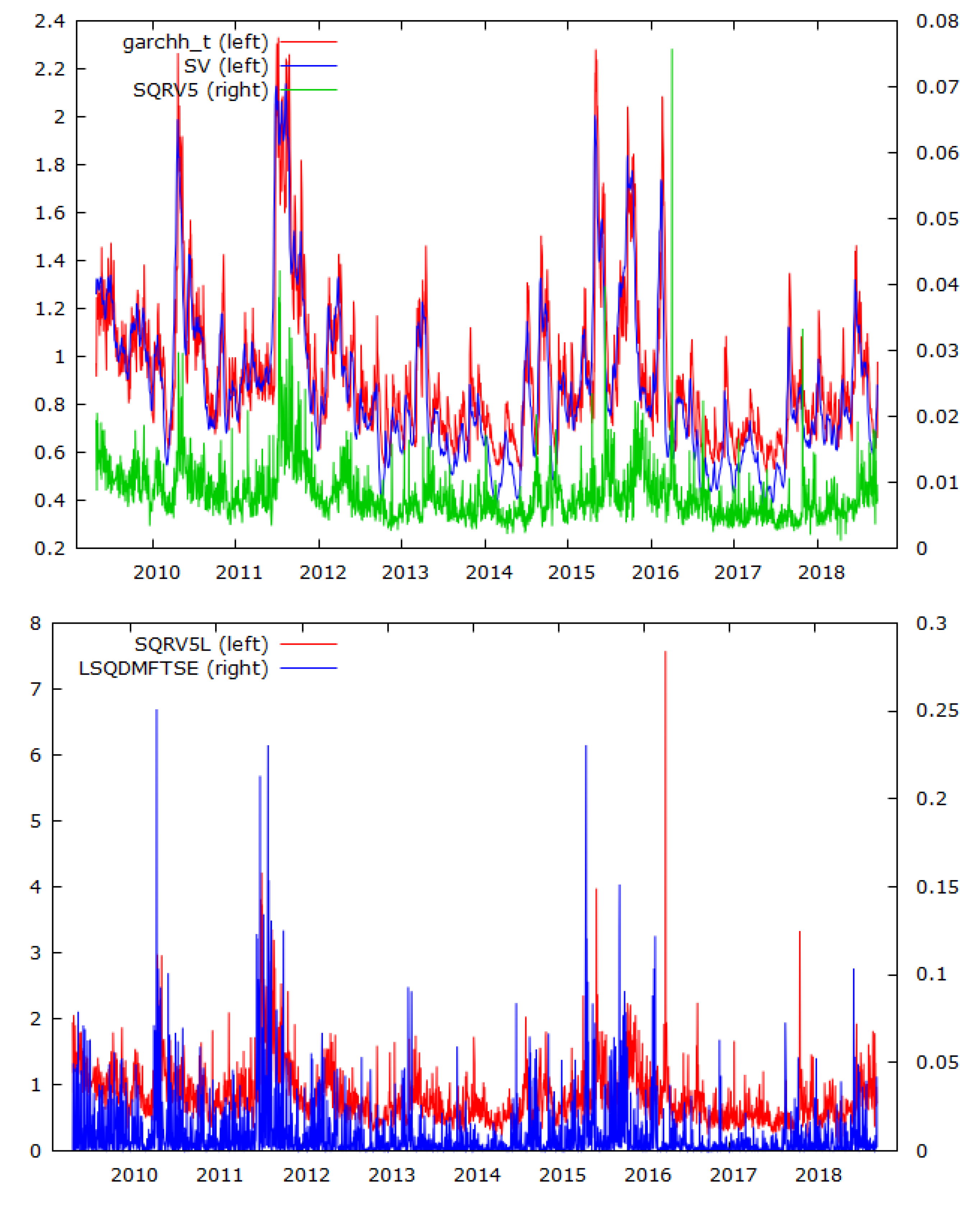
Summary statistics using 27 April 2009–16 April 2019 observations
for SQRV5L variable (2454 valid observations)
MeanMedianMinimumMaximum
0.819890.718370.115437.5756
Std. Dev.C.V.SkewnessEx. kurtosis
0.436440.532313.373629.966
5%95%IQ RangeMissing obs.
0.377371.59900.446760
Table 4. Generalised Autoregressive Conditional Heteroscedasticity (GARCH) (1,1) fitted to FTSE returns.
CoefficientsStandard ErrorT Statistic
mu1.360 × 10 4 1.601 × 10 4 0.850
omega3.406 × 10 6 8.087 × 10 7 4.211 ***
alpha11.199 × 10 1 1.728 × 10 2 6.939 ***
beta18.443 × 10 1 2.240 × 10 2 37.688 ***
Note: *** significance at 1% level.
Table 5. Regression analysis of three volatility models: SV, GARCH(1,1), and lagged demeaned squared returns.
Ordinary least squares (OLS) using 27 April 2009–16 April 2019 observations (T = 2454). Dependent variable: SQRV5L.
CoefficientStd. Errort-ratiop-value
const0.3057520.022582513.540.0000
SV0.5899300.024270024.310.0000
Mean dependent var0.819888S.D. dependent var0.436435
Sum squared resid376.5133S.E. of regression0.391859
R 2 0.194171Adjusted R 2 0.193842
F ( 1 , 2452 ) 590.8287p-value(F)4.1 × 10 117
Log-likelihood−1182.037Akaike criterion2368.075
Schwarz criterion2379.686Hannan–Quinn2372.294
ρ ^ 0.503365Durbin–Watson0.991133
OLS using 27 April 2009–16 April 2019 observations ( T = 2454). Dependent variable: SQRV5L.
CoefficientStd. Errort-ratiop-value
const0.2237660.02510938.9120.0000
garchh_t0.6451160.025805125.000.0000
Mean dependent var0.819888S.D. dependent var0.436435
Sum squared resid372.3346S.E. of regression0.389678
R 2 0.203114Adjusted R 2 0.202789
F ( 1 , 2452 ) 624.9784p-value(F)4.6 × 10 123
Log-likelihood−1168.344Akaike criterion2340.687
Schwarz criterion2352.298Hannan–Quinn2344.906
ρ ^ 0.490865Durbin–Watson1.015052
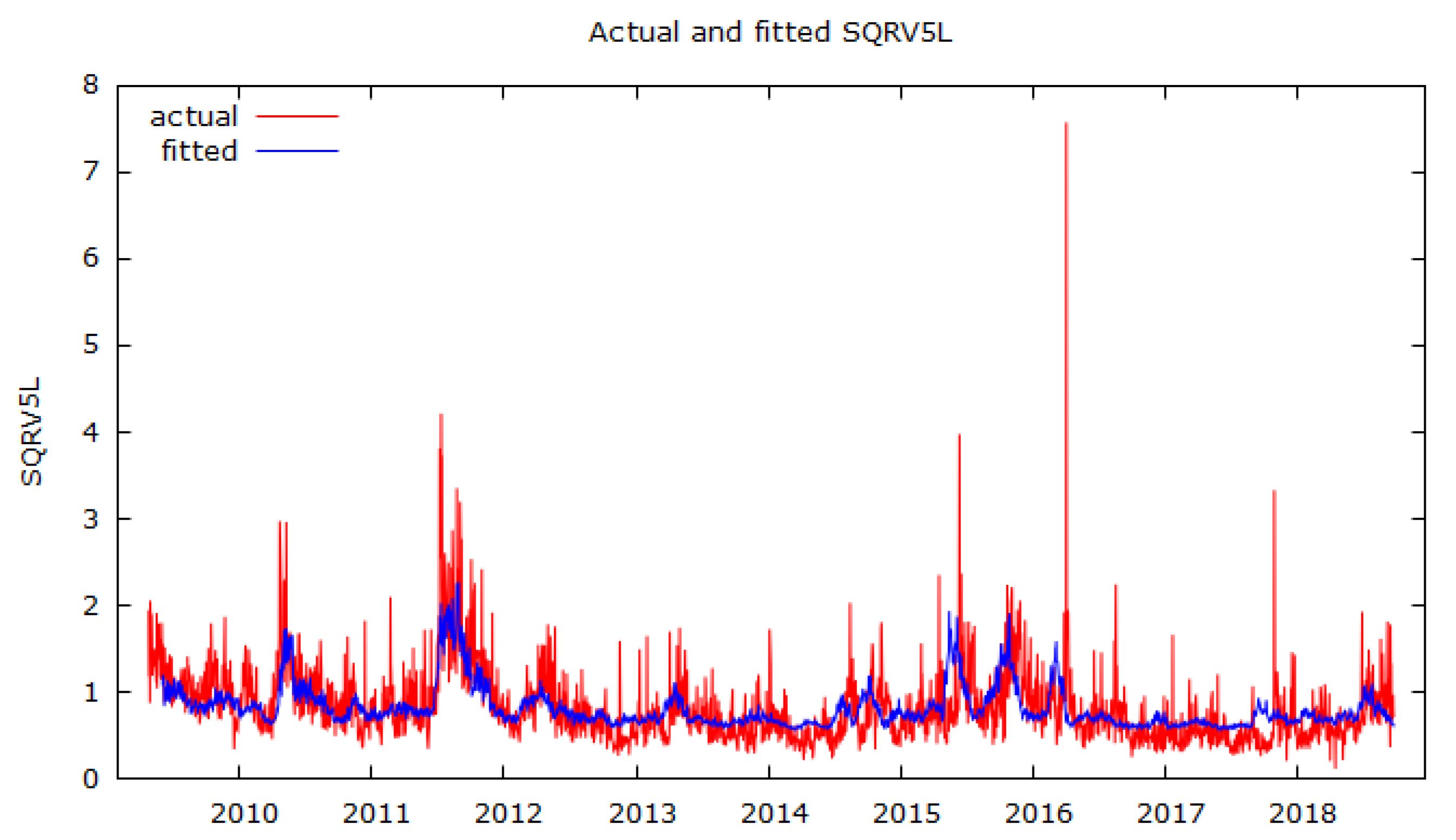
OLS using 4 June 2009–16 April 2019 observations ( T = 2426). Dependent variable: SQRV5L.
CoefficientStd. Errort-ratiop-value
const0.5446290.011189048.680.0000
LSQDMFTSE_10.4339340.4149771.0460.2958
LSQDMFTSE_20.5152500.4191021.2290.2190
LSQDMFTSE_31.180290.4200512.8100.0050
LSQDMFTSE_40.8396490.4218071.9910.0466
LSQDMFTSE_51.359510.4230133.2140.0013
LSQDMFTSE_60.1025260.4229700.24240.8085
LSQDMFTSE_70.6635050.4231771.5680.1170
LSQDMFTSE_80.2424770.4219540.57470.5656
LSQDMFTSE_91.583510.4232493.7410.0002
LSQDMFTSE_100.7151480.4229941.6910.0910
LSQDMFTSE_111.724720.4217904.0890.0000
LSQDMFTSE_122.431110.4224965.7540.0000
LSQDMFTSE_132.116990.4224705.0110.0000
LSQDMFTSE_140.6671810.4223791.5800.1143
LSQDMFTSE_152.049570.4222714.8540.0000
LSQDMFTSE_160.4386590.4220711.0390.2988
LSQDMFTSE_170.9942730.4217862.3570.0185
LSQDMFTSE_180.4307270.4209741.0230.3063
LSQDMFTSE_191.060330.4207992.5200.0118
LSQDMFTSE_200.01702700.4210310.040440.9677
LSQDMFTSE_211.037500.4196582.4720.0135
LSQDMFTSE_220.3038990.4208130.72220.4703
LSQDMFTSE_230.8422990.4200282.0050.0450
LSQDMFTSE_241.126940.4199052.6840.0073
LSQDMFTSE_250.8347490.4186371.9940.0463
LSQDMFTSE_260.7466050.4162431.7940.0730
LSQDMFTSE_271.925390.4151254.6380.0000
LSQDMFTSE_282.028310.4115774.9280.0000
Mean dependent var0.812434S.D. dependent var0.432184
Sum squared resid312.0871S.E. of regression0.360831
R 2 0.310989Adjusted R 2 0.302940
F ( 28 , 2397 ) 38.63918p-value(F)6.2 × 10 171
Log-likelihood−954.8254Akaike criterion1967.651
Schwarz criterion2135.677Hannan–Quinn2028.745
ρ ^ 0.429918Durbin–Watson1.139917
Table 6. Quantile-regression results of SQRV5L regression on lagged SV, lagged GARCH and lagged DMSQFTSERET Quantile estimates, using 27 April 2009–16 April 2019 observations (T = 2454). Asymptotic standard errors assuming independent and identically distributed (IID) errors.
VariableTauCoefficientStd. Errort-Ratio
SV(-1)0.050.001793840.0001948079.20827 ***
SV(-1)0.250.003869220.00017988321.5097 ***
SV(-1)0.500.005589580.00019958128.0066 ***
SV(-1)0.750.007464450.00027941526.7146 ***
SV(-1)0.950.01175190.00079812414.7245 ***
GARCHh_t(-1)0.050.001597550.0001958068.15884 ***
GARCHh_t(-1)0.250.004205790.00019181921.9259 ***
GARCHh_t(-1)0.500.006272050.00020411330.7283 ***
GARCHh_t(-1)0.750.008734170.00033419326.1351 ***
GARCHh_t(-1)0.950.01359440.00086026915.8025 ***
DMSQFTSERET(-1)0.050.01329120.003103504.28266 ***
DMSQFTSERET(-1)0.250.03224160.003502329.20578 ***
DMSQFTSERET(-1)0.500.04022090.0031183612.8981 ***
DMSQFTSERET(-1)0.750.05227370.005669669.21991 ***
DMSQFTSERET(-1)0.950.07378640.01401495.26486 ***
Note: *** significance at 1% level.

