Option Implied Stock Buy-Side and Sell-Side Market Depths

Department of Finance, Asia University, Taichung City 41354, Taiwan
Risks 2019, 7(4), 108; https://doi.org/10.3390/risks7040108
Submission received: 9 August 2019
/
Revised: 14 October 2019
/
Accepted: 23 October 2019
/
Published: 28 October 2019
(This article belongs to the Special Issue Measuring and Modelling Financial Risk and Derivatives)
Abstract
:This paper investigates option valuation when the underlying market suffers from illiquidity of price impact. Using option data, I infer trading activities and price impacts on the buy side and the sell side in the stock market from option prices across maturities. The finding displays that the stock market is active when the stock prices plummet, but becomes silent after the market crashes. In addition, the difference of option implied price impacts between the buy side and the sell side, which indicates asymmetric liquidity, increases with the time to maturity, especially on the day of the market crisis. Moreover, investors have different perspectives on the future liquidity after liquidity shocks when they are in a bull market or in a bear market according to the option implied price impact (or market depth) curves. I also calibrate three market indices simultaneously and reach the same conclusion that the three markets become erratic on the event date and calm down in the aftermath.
1. Introduction
Market liquidity refers to how easy it is to trade a security in the market. The sources of (il)liquidity mainly stem from four areas (Amihud et al. 2013). The first source of liquidity is exogenous transaction costs, such as brokerage and managerial fees, order-processing costs, taxes, etc. The second source of liquidity is demand pressure and inventory risk. The demand pressure, which results from the excess demand or excess supply of a security, leads to the price moving to the unfavored side. On the other hand, inventory risk is taken by the market maker regarding the exposure to price variation in his inventories. Inventory risks decide the tendency of the market maker to provide liquidity. The third source of liquidity is private information, which exists in two forms: the first is information about the fundamentals of a security, and the second is in regards to market activities; for example, a trading desk knows that a hedge fund is going to unload a huge position in the market. The last source of liquidity is search costs which commonly occur in over-the-counter (OTC) markets in which there is no central marketplace. Lacking an organized exchange platform, traders in OTC markets find their counterparties through brokers or dealers and this will cost them service fees and force them to accept worse term prices or to spend a lot of time liquidating their positions in order to negotiate with the counterparty that they eventually find.
Since liquidity is a vague concept and has multiple facets, it is difficult to use a unique measure to capture all sources of illiquidity. A widely adopted definition of liquidity is based on Kyle (1985) according to the following three dimensions. First, the market shows tightness if its bid-ask spread is small. Second, if a large amount of a security can be traded in markets without affecting its price, then the market is liquid according to its market depth. Third, price resiliency is another measure for liquidity, which means how quickly price recovers to its fundamental value after suffering from a demand or supply shock.
Based on the above definition, there are many measures of liquidity and liquidity risk used in research and in industries. The measures to inspect the tightness of the market are the quoted bid-ask spread, the proportional bid-ask spread, the effective bid-ask spread, the proportional effective bid-ask spread, etc. To measure the market depth, Kyle’s lambda, quoted depth, Amihud’s illiquidity measure (ILLIQ), order imbalance, etc. are commonly employed. Roll’s measure and the measure created by Pastor and Stambaugh (2003) can be used to capture market resiliency. Besides illiquidity in stock and bond markets, derivatives markets themselves have illiquidity and liquidity risk problems (Christoffersen et al. 2018). The sources of illiquidity in derivatives markets are similar to those in stock or bond markets. The distinct attribution of derivatives markets is their net supply is zero, while stock and bond markets have positive net supplies.
This paper focuses on illiquidity of limited market depth in stock markets and further derives option pricing under the existence of the buy side and the sell side price impacts in stock markets. People trade to invest, to borrow, to exchange assets, to hedge risks, to distribute risks, to gamble, to speculate, or to deal (Harris 2003). Under the limited depth of the market, the effect of executing a market order on prices is referred to as the price impact. In real markets, buyers can submit either a market order to buy at the ask price or a limit order to wait at the bid price and sellers can act in the opposite direction. Because of random arrivals of buyers and sellers and different types of orders, the liquidity is generally uncertain. Hence, I define the random price impacts caused by time-changing order flows hereafter as the liquidity risk. As Professor Engle elaborated in his Nobel lecture (Engle 2004): “A large or medium size buyer will raise prices, at least partly because market participants believe he could have important information that the stock is undervalued. This effect is called the price impact and is a central component of liquidity risk, and a key feature of volatility for ultra-high frequency data.” Since the price impact of (large) traders will lead to jumps in stock prices, the success of Levy processes in modeling underlying assets consolidates the ubiquity of price impacts.
Based on above argument, I integrate the above liquidity risk and volatility risk in general option pricing models. The stochastic arrival of order flows leads to liquidity risk and short-term volatility risk as well. Long-term volatility is modeled as a mean-reverting square rooted process which captures the changes in fundamental values. In a way that differs from the previous microstructure perspective (e.g., Brennan and Subrahmanyam 1996), I directly link time-changing information flows to random order flows which is similar to the information risk of Easley et al. (2002). The idea to model random order flows is originated from uncertain demand and supply of the underlying assets which make replicating or hedging options difficult. In particular when market catastrophes occur, most investors are focused in the same trade direction and they unavoidably face large price impacts. The main feature of this paper is that I separate the effects of order flows into those that are buyer-initiated and those that are seller-initiated and analyze the market depths for both sides. The price impact of buying one share or selling one share of the stock is intuitively different and this phenomenon may be explained by distinct trade motivation or information content owned by traders. It also reflects investors’ inclination to provide liquidity.
Option pricing in illiquid markets is an important issue in the real world. The developments in option pricing with price impacts focus on analyzing trading strategies for a large trader whose sizable transaction will move the price (e.g., Cetin et al. 2004, 2006). When facing a stochastic supply curve of the underlying asset, Cetin et al. (2004) proposed that the self-financing trading strategy of a large trader is to slice small orders to avoid liquidity risk. They develop an option pricing model in an “approximately” complete market and derive a Black-Scholes style formula. Furthermore, Cetin et al. (2006) applied the above model in an empirical study and discussed practical issues when trades are discontinuous and hence when the market is incomplete. Option valuation is related to replicating portfolios with the minimum liquidity costs using dynamic programming.
The work of Cetin et al. (2004, 2006) did not take stochastic liquidity into serious consideration because they only discussed temporary price impacts and small trade sizes. Moreover, they did not consider the situation where the stochastic volatility of the stock price and possible jumps in prices or volatilities prove that it is very important in option pricing models (see Bakshi et al. 1997). It is also intuitive that the strategy of using the infinitesimal trading size is neither feasible in discrete time markets nor optimal in market crash periods.
Another research direction discusses the relationship between information and price volatility because information is a critical component and incentive when it comes to trading and volatility is the central factor of option pricing (e.g., Chang et al. 1998). Clark (1973) introduced a subordinator, the trading volume, into the stock price process and conjectured that the stock price follows log normal conditioning on cumulated trading volumes. The empirical work of Ane and Geman (2000) suggested that the cumulated number of trades is the subordinator which recovers the log-normal stock price process. Several articles relate information time to option pricing including Chang et al. (1998), and Jagannathan (2008). Chang et al. (1998) used a Poisson process to model the information time and Jagannathan (2008) referred the information time to economic shocks in macroeconomic circumstances.
In a way that is different from previous studies, I adopt normalized trade size to build information time. Changing calendar time to information time in the underlying price process gives an alternative description of the price impacts of order flows in the price process. This time change not only makes my problems tractable and solvable but also provides a built-in dependence for multivariate models, i.e., the situation of flight to liquidity or the commonality of illiquidity. The later benefit of this approach is that my models may easily be extended to accommodate multivariate option pricing with market-wide liquidity shocks. In addition, market prices of options provide valuable information regarding the liquidity of underlying assets. Similar to the implied volatility obtained from an option’s market price and the implied default probability inferred from the market price of the credit default swap, I can also acquire (risk neutral) implied market depth from the market prices of options. If an investor wants to make a sizable trade, the market depth is critical information and this information is partially revealed in the order book. Therefore, it is desirable to have market depth information derived from option trades as occurs in my model.
I contribute to the literature in at least three aspects. Firstly, I construct flexible option pricing models to incorporate stochastic liquidity, volatility, and leverage effect and to extend to multi-asset situations. Secondly, using intraday stock data or daily option prices, I find a consistent result of asymmetric buy-side and sell-side stock market depths. Lastly, calibrated to market option prices of different maturities, option-implied market depths in buy side and sell side show distinct changes with time in market crashes such as the 9/11 terrorist attack. The trading activities inferred from option prices increase for all maturities on the event days. This implies that the traders anticipate more trades in the short run but a widening difference between buy-side and sell-side market depths in the future in the catastrophes.
The remainder of this paper is organized as follows. In Section 2, I propose a continuous time stochastic volatility-liquidity option pricing model. The extension and valuation are also included. Section 3 presents the empirical data, estimation methods and calibration. The implementation results are listed in Section 4. I conclude the paper in Section 5.
2. Model
2.1. The Economic Foundations
The trading mechanisms of securities markets generally follow one of two types, namely, quote-driven markets and order-driven markets. In both kinds of markets, the forces that drive prices come from the demand for and supply of stocks. From the viewpoint of the liquidity aspects, the liquidity supply comes from the market makers in quote-driven markets while traders using limit orders play the role of liquidity supplier in order-driven markets. The liquidity demanders are those who submit market orders at the expense of immediacy prices. Generally speaking, impatient traders are inclined to use market orders and patient traders are likely to adopt limit orders.
The price behavior of the stock is decided by the balance of the buying force and the selling force at any instant in time. I say that the buying force consists of the cumulated trades that drive up the price and the selling force comprises the cumulated trades that drive the price down. To buy a share of stock, the price is settled by the equilibrium of demand and supply in the buy side market. The liquidity supplier will set different prices for different quantities of demand and this constitutes a supply curve in the buy side market. The sell side market has the same structure. A slightly distinct argument is that the price concession for buying one share does not equal the discount for selling the same amount. In essence, I have different market depths in the two side markets.
Therefore, I let be the process of cumulated market buy orders and be the arriving buy order at time . Similarly, is the process of cumulated market sell orders and is the arriving sell order at time . Suppose that market buy orders are satisfied by limit sell orders and that market sell orders are filled up by limit buy orders. At any instant of continuous time, the market processes either a market buy order or a market sell order. The market clearing condition on both sides determines the equilibrium stock price.
2.2. Parsimonious Stochastic Volatility-Liquidity Models
2.2.1. A stochastic Liquidity Model (SL)
If the stock price behavior is described by the aggregation of trading activities, such as order flow-driven activities, the price process can be modeled as follows
where I assume that is a gamma process with mean and variance rate . An economic exposition is that is the buying force originating from the cumulative buyer-initiated orders which bids up the price at time and is the simultaneous selling force generated by the cumulative seller-initiated orders which pushes the price down. The balance of two forces at time is denoted by . According to the assumption of linear supply curves, I have the normalized buyer-initiated order flow at time (trade size divided by shares outstanding, i.e., turnover) which is proportional to the log price increment produced by the buying force, i.e., . Similarly, the scaled seller-initiated order flow can be expressed as . Putting the two forces together, the change in the log stock price at time may be expressed by . Thus, the level of the price slippage is measured by the price impact coefficients, i.e., is the buy-side market depth and is the sell-side market depth. They are like the slopes of supply curves inferring the price change for buying or selling one unit of a stock.
To sum up, the price process evolves as
The second equality assumes that the cumulated buyer-initiated and seller-initiated order flows belong to two copies of gamma processes , where is a standard gamma process of unit mean and variance. The equilibrium behavior of the stock price can be explained because there are two heterogeneous groups who exchange their information through trades. The balance of two forces modeled by the difference between two gamma processes gives rise to a jump stock price process of infinite activity but of finite variation, and this is the well-known variance gamma (VG) process.
Another version of a variance gamma (VG) process is expressed as a Brownian motion with the drift term, but the time is changed as a standard gamma process as follows . The time change effectively transforms the calendar time to the business time (or the economic time) , which is meaningful in describing market activities. This corresponds to the order flow process in my model setting.
Since and measure the market illiquidity, indicates that the downside market is more illiquid. This may also explain why liquidity providers charge a higher premium on downside risk. Additionally, it represents the rate of market trading activity and hence when many assets or indices use the same to express the factor (commonality) of market liquidity risk, it means that these assets are more exposed to the market liquidity risk if the market activity rate is higher (high beta). This is similar to the one beta in the model of Acharya and Pedersen (2005).
The model is flexible to adding the drift term into the price dynamics as follows
where represents a “convexity correction.” To distinguish the parameters under the statistical measure from those under the risk neutral measure, I denote the parameters with apostrophes, and (i.e., buy and sell price impact coefficients respectively) are under the statistical measure. Therefore, the risk neutral dynamics for the stock price follows
where . The corresponding characteristic function is as follows
where .
2.2.2. A Stochastic Volatility-Liquidity Model (SVL)
The stock price movement described above only captures the short-term price behavior caused by trading activities and it fails to explain the option prices of all maturities. One possible improvement is to include the stochastic volatility factor which successfully apprehends the long-term changes of fundamental values in the model. With stochastic volatilities, the phenomenon of volatility clustering can be captured by the model. To incorporate the effect of stochastic volatility, I have to add a stochastic time change in the above process as follows
where is the random time and the variance rate follows a mean-reverting square root process (CIR process) as
where is the mean-reverting rate, is the long-term variance level and is the volatility of the variance rate. The risk neutral price process is then written as follows by a mean-correcting argument
The characteristic function of the log stock price is hence obtained
where
The price process in the SVL model is similar to that of the stochastic liquidity-volatility model of Watanabe (2007) whose continuous-time version of the price process evolves as
Distinct from SVL, he adopted a GARCH process to model volatility and focused only on the information shock to liquidity and volatility.
2.2.3. A Stochastic Volatility-Liquidity Model with the Leverage Effect (SVLL)
The SVL model assumes that the underlying price process is independent of the second time-changed process. However, it is well known (see Black 1976) that volatilities usually increase when stock prices drop, i.e., there is the so-called leverage effect. To incorporate the leverage effect, I adopt the method of Carr et al. (2003) to model the price process as follows
where measures the correlation between the stock price and its variance rate. Under this price process, I have the corresponding characteristic function as follows
where
2.3. Short Summary
The intuition underlying my models is to take order flow risk as the source of liquidity risk. Therefore, large order flow rates mean more frequent trading activities, with the result that more information arrives in the markets. Option pricing in stochastic volatility and liquidity environments needs to consider both the order flow risk and the volatility risk. Therefore, I expect that the option valuation will depend on those parameters driving order flow rates and variance rates.
2.4. Extension
In the following model, the parameter beta in the time change plays the role which globally affects information arrival rates and hence the market liquidity risk. Luciano and Schoutens (2006) used this approach to calibrate financial products due to market or credit risks. I have applied it to a market with liquidity risk.
A multi-asset/multi-market SVLL model with flight to liquidity (MSVLL) is set up as follows:
where denotes the asset. I take the stochastic time change as a systematic liquidity shock and the parameter as a market-wide liquidity risk factor. This common factor can cut off the order flows of each asset simultaneously and hence make the market calm down.
2.5. Generalization
The drawback in previous settings is I assume that the normalized cumulative buyer and seller order flows follow the same gamma processes. To release this restriction, I can employ the two order flow processes evolve as two distinct non-decreasing Levy processes. In mathematical terms, I write the two processes as follows
Therefore, the risk-neutral price process with stochastic volatility and leverage effect is
where is the cumulant exponent of a Levy process .
2.6. Valuation
I have already obtained the closed form characteristic functions of the three models in the above subsection. Therefore, I can apply the faster Fourier transform (FFT) introduced in Carr and Madan (1999) to the option pricing in my framework. The corresponding option prices can be expressed as
where .
3. Data and Methodology
First, to show that the proposed stock price process is capable of capturing the two-side price impacts of stock trades, I examine the price impacts of the buy orders and the sell orders from the stock tick data and compare the result with the two-side price impacts derived from my setting stock price process from daily stock data. I acquire the intraday transaction data from NYSE TAQ and daily stock prices from CRSP for the following six companies that differ in size in different industries for investigation: International Business Machines (IBM), Coca Cola (KO), Fedex (FDX), Barnes & Noble (BKS), Boeing (BA), and Disney (DIS). Since I do not consider option market illiquidity itself, I choose these underlying stocks whose options are highly liquid. Second, I calibrate option pricing models to option data from OptionMetrics. To be specific, I estimate the parameters, especially stock liquidity measures, in different model settings from option prices of three main market indices (SPX, DJX, and NDX) during January to June in 2007. Lastly, I compare the changes of option implied stock liquidities across option maturities before, during and after two significant events to see how markets anticipate the market activities and market depths in the short run and in the long run.
3.1. Data Description
The trade and quote data are downloaded from the NYSE TAQ in WRDS (Wharton Research Data Services) covering the period from 3 January 2007 to 31 March 2007. I retain only NYSE trades extending from 9:30 am through 4:00 pm each day and remove abnormal and nonstandard trades following Hasbrouck (2007). To label each order as being buyer-initiated or seller-initiated, I match trades and quotes based on the principle of a two-second time lag between trade and quote and give each trade a sign following the classification rule of Lee and Ready (1991). I also obtain the numbers of shares outstanding from Compustat in WRDS for normalization necessity.
To calibrate the options data, I retrieve raw data from Ivy OptionMetrics in WRDS and the criteria used to filter the data may be described as follows. I select three main index call options in the United States, namely, DJX, NDX, and SPX. For each month, I choose the mid-month Wednesday as being representative of that month, and the days selected are 17 January, 14 February, 14 March, 11 April, 16 May, and 13 June in 2007. I adopt the LIBOR as the risk free rate obtained from the Federal Reserve Bank of St. Louis. To assign the risk free rate for each maturity, I interpolate the two LIBOR rates which are the closest to that maturity. The dividend yields are also obtained from OptionMetrics. I calculate the option prices as the mid prices of the best bid and best offer prices. Only best bids and bid-ask spreads greater than zero are kept. Those option prices less than 3/8 that violate the basic arbitrage restrictions are eliminated. I also discard deep out of or deep in the money options and only keep those for which moneyness lies within the range . Options with time to maturity of less than seven days or longer than one year are not included in my sample.
I pick two event days, namely, 17 September 2001 (the first trading day after the 9/11 terrorist attack), on which the three index prices slid by more than 3%, and 27 February 2007 (the inception date of the subprime crisis), which triggered a one-day drop in the Dow Jones Industrial Average of 3.3%, the largest decline since the 11 September 2001 attacks. To compare the changes in the markets, I open event windows [−1, 1], i.e., I add 10 September 2001 and 18 September 2001 for the first event day and 26 February 2007 and 28 February 2007 for the second event day, and include them in my investigation. The options for these six additional days of event studies follow the same filtering principle as stated above. I am also interested in the changes in term structures during these windows. To maintain enough data for the term structure studies, I only discard option prices that are less than 1/8. The other rules are not changed.
3.2. Methodology
This section illustrates estimation and calibration methods in this study. I explain how to estimate price impact coefficients from intradaily stock data and how to estimate price impact parameters in stock price process from daily stock data using the maximum likelihood approach. I also show how to calibrate parameters in option pricing models by minimizing pricing errors.
3.2.1. Estimation for Illiquidity in Intraday Markets
To estimate the price impact coefficients or market depths, I adopt the intraday transaction data from NYSE TAQ. The first step is to sign each order as a buyer-initiated order or a seller-initiated order. I follow the Lee and Ready algorithm to give a sign for each trade as mentioned in the data descriptions. To analyze the market impacts on the buy side and on the sell side, I run a regression of the log return on the size of the normalized buyer-initiated order flow (using total shares outstanding to normalize) and on the size of the normalized seller-initiated order flow, respectively, as follows1
where denotes the constant term, is the normalized buyer-initiated order flow and is the normalized seller-initiated order flow at time and is the error term of the regression. In the equation, scales the market depth on the buy side and measures the market depth on the sell side.
3.2.2. Estimation for the Behavior of Statistical Price Process
On the other hand, I estimate the parameters in the statistical dynamics of the price process in the SL model. The density function of the variance gamma process is
with and as the modified Bessel function of the second kind (the integral formula refers to Appendix A). To obtain the estimates of the statistical density parameters for the daily returns, I adopt the maximum likelihood approach. The implement is straightforward.
3.2.3. Calibration of Option Models
I calibrate the model parameters with the market prices of options using the weighted root mean square error (RMSE) as follows
It is quite intuitive to choose the inverse of the bid-ask spreads as weights, since I want to attach higher weights to (more liquid) options with narrow spreads. The nonlinear least squares method2 is then applied to minimize the root mean square errors. I calibrate the model parameters by setting the maximum number of iterations up to 20,000 times to avoid early termination. Other measures such as the average absolute error as a percentage of the mean price (APE), the average absolute error (AAE), and the average relative percentage error (ARPE) are also calculated as estimates of the goodness of fit (see Schoutens 2003).
4. Results
4.1. Estimates in Intraday Markets
Table 1 exhibits the estimation results of the market depths in intraday data for the six chosen companies. The estimated market impact coefficients on the buy side are smaller than those on the sell side for all companies and all of them are significant. All companies, regardless of their size and the industry they belong to, have deeper market depths on the buy side. This result validates the fact that the downside market is more illiquid in terms of high frequency data.
4.2. Estimates in Daily Markets
Table 2 lists the results of the maximum likelihood estimators and their Hessian standard errors. The implied market depths of the six companies are displayed in Table 2 as well. The results show that four of the six companies have smaller market impact coefficients on the buy side. The two exceptions are Barnes & Noble and Disney which have deeper sell side markets, but their likelihood values are relatively small. All estimated parameters are significant according to their p values.
4.3. Calibration in Index Option Markets
The calibrations of the option prices for the Black-Scholes, SL, SVL, SVLL, and MSVLL models are presented in Table 3. The findings show that the SVLL model has the smallest RMSE for the single index calibration, i.e., the stochastic volatility and liquidity model with leverage effects is the best candidate for the stock price process. Capturing additional sources of uncertainty appears to have a considerable effect on option prices and demonstrate a significant pricing improvement (Abudy and Izhakian 2013). On average, I also have smaller sell side market depths. This means that the market forecasts that investors are less willing to provide liquidity for sellers. The second part of Table 3 exhibits the joint calibration of the three main market indices in the United States. The dependence of the three indices is captured by one parameter which scales the rate of information arrivals. This result also shows that all three markets on average have deeper market depths on the buy side.
4.4. Event Days
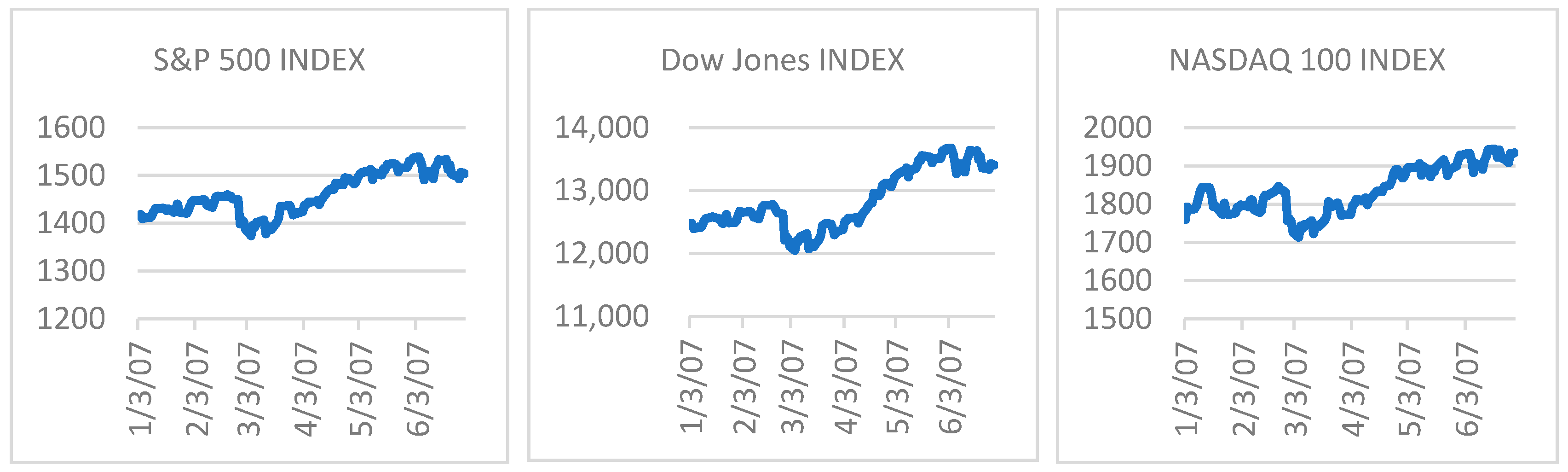
To pin down the event point of the warning signal in the subprime crisis, Figure 1 displays the price levels for the three market indices in my period under investigation. All prices fell by more than three percent on 27 February 2007. Therefore, it is interesting to see the changes in market conditions, especially those implied (risk neutral) market depths based on the market prices of options. Price movements in this six-month period exhibit an upward moving trend although prices decline sharply on 27 February. I also evaluate the implied market depths in market option prices during another event, the 9/11 terrorist attack, for comparison purposes.
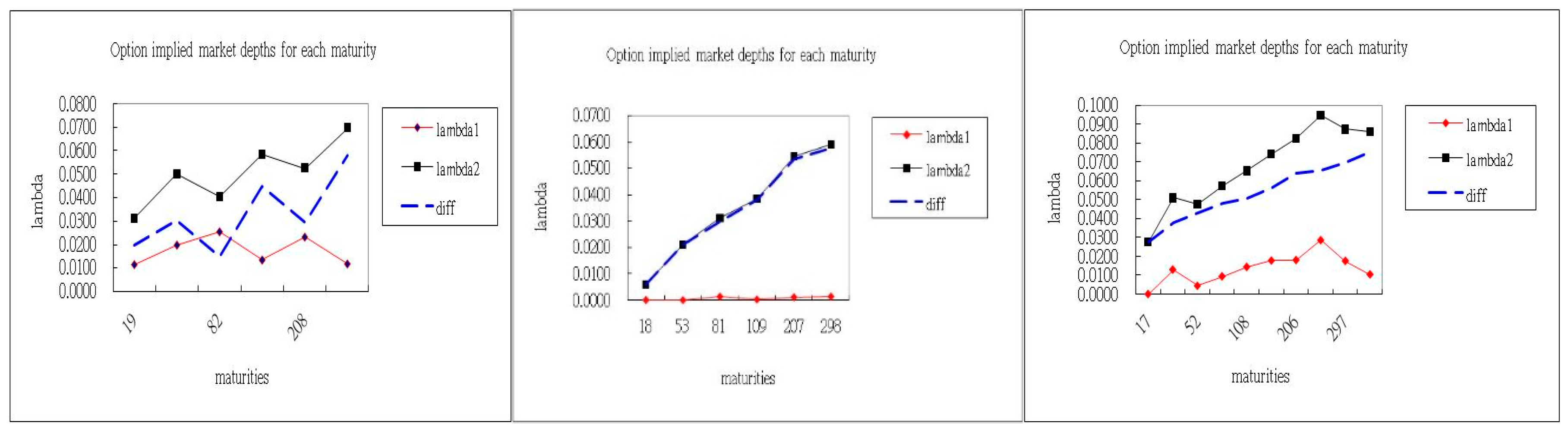
Figure 2 shows the term structures of risk neutral implied market depths on the buy side and on the sell side from 26 February 2007 to 28 February 2007. The sell side price impact curve always lies above the price impact curve on the buy side. The difference between the buy side market depth and the sell side market depth, i.e., the market depth spread, becomes greater for longer maturities. This situation was particularly significant on 27 February 2007. This market depth spread curve is similar to the yield curve in a sense that the market depth spread in the long term is much sensitive to liquidity shocks. This is also consistent with the finding of Chacko et al. (2008) that immediacy prices for buyers become much more elastic and the immediacy prices facing sellers are less elastic during liquidity events.
Table 4 illustrates the market activities of the three main market indices during the event. I find that on that day the stochastic clock denoted by beta runs faster compared with the previous day which means trading was brisk, more information arrived and there was a higher order flow rate on the event day. High beta also induces the market more volatile which shows a panic and high sensitivity to any pieces of information. The implication of higher market activity rates could be that more people hold heterogeneous beliefs and information such that they trade more frequently than they do in normal markets. However, markets became quiet and trading was light since the economic time slowed down on 28 February 2007.
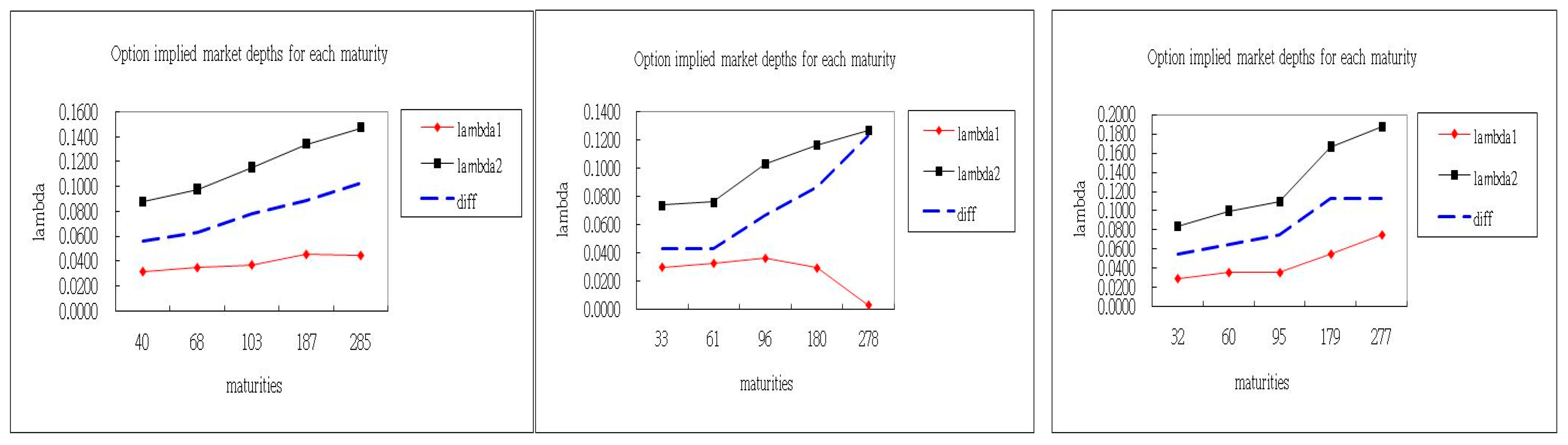
In the history of financial crises, an unpredictable market crash occurred on 11 September 2001. Compared with the other event examined which resulted from the macroeconomic early warning of the subprime mortgage crisis, a terrorist attack had never taken place before, even though there was still a similar term structure pattern of implied market depths on both event days (see Figure 3). On the first transaction day after the terrorist attack, the implied buy side market depth increased with longer maturities and the implied sell side market depth decreased with longer maturities. However, after the collapse, uncertain marketability levels caused both price impact coefficients to go up. One possible explanation for the phenomenon of the widening difference between the market depths on the two sides on the event day could be that more people were willing to sell but fewer wanted to buy, and hence market depth on the buy side became deeper and the differences in market depths increased.
4.5. Market-to-Model
Table 5 explains that overall trade frequencies are higher on 17 September 2001. After the event, liquidity measured by trading activities and market depths shows that market liquidity dried up suddenly. In addition, I find that pricing errors decrease on the day of the event, especially for near-to-maturity options. This can be explained as the market shocks bring the market prices from mark-to-market back to mark-to-model.
4.6. Comparison between Two Events
It is worth comparing the market reactions for the two different events. I find that the common features are the high market activity and the increasing differences in the term structure for the market depths of the two sides on the event days. It is noteworthy that the price impact curve on the buy side became positively sloped on the second trading day following the terrorist attack. This implies that the traders on both sides expected the markets to be less liquid in the future. Recall that the market trend in the first half year of 2007 was upward moving and hence this distinct feature shows that markets behave differently and have diverse perspectives in the bull market as well as in the bear market.
4.7. Short Summary
Empirically, I find the following evidence. First, both the intraday and daily data indicate that the buy side market is deeper than the sell side market. Secondly, the term structures of option implied market depths infer that the difference between the market depths on the two sides increases significantly with maturity when prices plummet. This difference is more pronounced for long-term liquidity. Thirdly, the information flow rate is high when a market collapses, but slows down after the event. Fourthly, option pricing errors decrease on the event day, especially for short-term maturities options. Lastly, all tests show that market activity rates temporarily increase on the day of market crash.
4.8. Implication for Asymmetric Liquidity
Brennan et al. (2012) examine the long-term high-frequency data and indicate that there exists asymmetric liquidity significantly as I find in this paper. There are four reasons to explain the phenomenon of asymmetric liquidity in a quote-driven market. The first two interpretations are based on the perspective of inventory risk and private information while the last two expositions are in terms of funding constraint of the market maker and short-selling restriction of the informed trader.
Firstly, since the market maker tends to hold positive inventories of the stock in which they make a market, a purchase order will reduce his inventory risk while a sell order will increase it. Secondly, if the market maker sells to an informed buyer he suffers an opportunity loss, but if he buys from an informed seller he will suffer an actual loss. Therefore, his price reaction to a sell order will be more extreme than to a buy order. Thirdly, market makers may face funding constraints for their inventory positions, and hence it is likely that sell trades from investors will face worse terms than buy trades. Lastly, the informed trader may be an insider of the company who holds net long shares. Because of costly short selling, sell orders are more likely to reflect private information than buy orders.
5. Conclusions
In this paper, I empirically examine the proposed stochastic volatility and liquidity option pricing model. The evidence indicates that selling one share costs more than buying one share on average. In addition, the information obtained from the options tells us that the market activity is erratic on the event day and the sell side market becomes more illiquid than the buy side market, especially based on a long-run perspective.
It would be compelling to further investigate a liquidity risk premium under this model setting in future studies. Specifically, we can back out a liquidity risk premium by comparing the estimates taken from high-frequency stock returns under P measure and from option prices under the Q measure. Obtaining the liquidity risk premium will be helpful to further understand several puzzles, such as the distress premium puzzle.
Funding
This research received no external funding.
Acknowledgments
I acknowledge two anonymous reviewers for their very useful comments. I also thank my Ph.D. supervisor, Mao-Wei Hung, and the dissertation committee members for their helpful comments and suggestions. All errors are my own.
Conflicts of Interest
The author declares no conflict of interest.
Appendix A
In this context, the statistical gamma process is slightly different from that in Madan et al. (1998). The density function for can be written as the conditional density given a realization gamma with the random variable integrated out as follows
Using the integral formula given by Gradshetyn and Ryzhik (1980), I have the density function for the log price relative in Equation (15)
References
- Abudy, Menachem, and Yehuda Izhakian. 2013. Pricing stock options with stochastic interest rate. International Journal of Portfolio Analysis and Management 1: 250–77. [Google Scholar] [CrossRef]
- Acharya, Viral, and Lasse Heje Pedersen. 2005. Asset pricing with liquidity risk. Journal of Financial Economics 77: 375–410. [Google Scholar] [CrossRef] [Green Version]
- Amihud, Yakov, Haim Mendelson, and Lasse Heje Pedersen. 2013. Market Liquidity: Asset Pricing, Risk, and Crises. Cambridge: Cambridge University Press. [Google Scholar]
- Ane, Thierry, and Hélyette Geman. 2000. Order flow, transaction clock and normality of asset returns. Journal of Finance 55: 2259–84. [Google Scholar] [CrossRef]
- Bakshi, Gurdip, Charles Cao, and Zhiwu Chen. 1997. Empirical performance of alternative option pricing models. Journal of Finance 52: 2003–49. [Google Scholar] [CrossRef]
- Black, Fischer. 1976. Studies of stock price volatility changes. In Proceedings of the 1976 Meetings of the Business and Economic Statistics Section. Washington: American Statistical Association, pp. 177–81. [Google Scholar]
- Brennan, Michael, and Avanidhar Subrahmanyam. 1996. Market microstructure and asset pricing: on the compensation for illiquidity in stock returns. Journal of Financial Economics 41: 441–64. [Google Scholar] [CrossRef]
- Brennan, Michael, Tarun Chordia, Avanidhar Subrahmanyam, and Qing Dong. 2012. Sell-order Liquidity and the Cross-Section of Expected Stock Returns. Journal of Financial Economics 105: 523–41. [Google Scholar] [CrossRef]
- Carr, Peter, and Dilip B. Madan. 1999. Option valuation using the fast Fourier transform. Journal of Computational Finance 2: 61–73. [Google Scholar] [CrossRef] [Green Version]
- Carr, Peter, Hélyette Geman, Dilip B. Madan, and Marc Yor. 2003. Stochastic volatility for Levy processes. Mathematical Finance 13: 345–82. [Google Scholar] [CrossRef]
- Cetin, Umut, Robert A. Jarrow, and Philip Protter. 2004. Liquidity risk and arbitrage pricing theory. Finance and Stochastics 8: 311–41. [Google Scholar] [CrossRef]
- Cetin, Umut, Robert A. Jarrow, Philip Protter, and M. Warachka. 2006. Pricing options in an extended Black Scholes economy with illiquidity: theory and empirical evidence. The Review of Financial Studies 19: 493–529. [Google Scholar] [CrossRef]
- Chacko, George C., Jakub W. Jurek, and Erik Stafford. 2008. The price of immediacy. The Journal of Finance 63: 1253–90. [Google Scholar] [CrossRef]
- Chang, Carolyn W., Jack S. K. Chang, and Kian Guan Lim. 1998. Information-time option pricing: Theory and empirical evidence. Journal of Financial Economics 48: 211–42. [Google Scholar] [CrossRef]
- Christoffersen, Peter, Ruslan Goyenko, Kris Jacobs, and Mehdi Karoui. 2018. Illiquidity premia in the equity options market. The Review of Financial Studies 31: 811–51. [Google Scholar] [CrossRef]
- Clark, Peter K. 1973. A subordinated stochastic process model with finite variance for speculative prices. Econometrica 41: 135–55. [Google Scholar] [CrossRef]
- Easley, David, Soeren Hvidkjaer, and Maureen O’Hara. 2002. Is information risk a determinant of asset returns? Journal of Finance 57: 2185–221. [Google Scholar] [CrossRef]
- Engle, Robert. 2004. Risk and volatility: Econometric models and financial practice. The American Economic Review 94: 405–20. [Google Scholar] [CrossRef]
- Gradshetyn, Izrail Solomonovich, and Iosif Moiseevich Ryzhik. 1980. Table of Integrals, Series, and Products. New York: Academic Press. [Google Scholar]
- Harris, Larry. 2003. Trading and Exchanges: Market Microstructure for Practitioners. New York: Oxford University Press. [Google Scholar]
- Hasbrouck, Joel. 2007. Empirical Market Microstructure: The Institutions, Economics, and Econometrics of Securities Trading. New York: Oxford University Press. [Google Scholar]
- Jagannathan, Raj. 2008. A class of asset pricing models governed by subordinate processes that signal economic shocks. Journal of Economic Dynamics and Control 32: 3820–46. [Google Scholar] [CrossRef]
- Kyle, Albert S. 1985. Continuous auctions and insider trading. Econometrica 53: 1315–36. [Google Scholar] [CrossRef]
- Lee, Charles M., and Mark J. Ready. 1991. Inferring trade direction from intraday data. Journal of Finance 46: 733–46. [Google Scholar] [CrossRef]
- Luciano, Elisa, and Wim Schoutens. 2006. A multivariate jump-driven financial asset model. Quantitative Finance 6: 385–402. [Google Scholar] [CrossRef] [Green Version]
- Madan, Dilip B., Peter Carr, and Eric C. Chang. 1998. The variance gamma process and option pricing. European Finance Review 2: 79–105. [Google Scholar] [CrossRef]
- Pastor, Ľuboš, and Robert F. Stambaugh. 2003. Liquidity risk and expected stock returns. Journal of Political Economy 111: 642–85. [Google Scholar] [CrossRef]
- Schoutens, Wim. 2003. Levy Processes in Finance: Pricing Financial Derivatives. West Sussex: John Wiley & Sons Ltd. [Google Scholar]
- Watanabe, Masahiro. 2007. A Model of Stochastic Liquidity. Yale ICF Working Paper No. 03-18; EFA 2003 Glasgow Annual Conference Paper. Available online: https://ssrn.com/abstract=413983 (accessed on 26 October 2019).
| 1 | I also run the following regression with fixed cost and the conclusion does not change: |
| 2 | The results are verified using the Nelder-Mead simplex approach as well as the simulated annealing method. |
Figure 1.
Price series of S&P 500 (left), Dow Jones (middle) and NASDAQ 100 (right) between 3 January and 30 June 2007.
Figure 1.
Price series of S&P 500 (left), Dow Jones (middle) and NASDAQ 100 (right) between 3 January and 30 June 2007.

Figure 2.
Option implied market depths for all maturities on 26 February (left), 27 February (middle) and 28 February (right) 2007.
Figure 2.
Option implied market depths for all maturities on 26 February (left), 27 February (middle) and 28 February (right) 2007.

Figure 3.
Option implied market depths for all maturities on 10 September (left), 17 September (middle) and 18 September (right) 2001.
Figure 3.
Option implied market depths for all maturities on 10 September (left), 17 September (middle) and 18 September (right) 2001.


Table 1.
Price impact coefficients in intraday data.
| Company Name | ||
|---|---|---|
| IBM | 0.0138 (9.45) | 0.1414 (50.61) |
| KO | 0.0320 (13.25) | 0.2064 (20.64) |
| FDX | 0.0433 (11.81) | 0.1859 (17.34) |
| BKS | 0.0994 (15.46) | 0.1814 (11.25) |
| BA | 0.0270 (20.27) | 0.2722 (38.90) |
| DIS | 0.0447 (26.16) | 0.2583 (45.71) |
The logarithmic return is regressed on the (normalized) buyer-initiated order flow and on the (normalized) seller-initiated order flow using NYSE TAQ intraday data. This table reports the regression coefficients which stand for the market depths on the buy side and on the sell side. The corresponding t-values are listed in the parentheses. The numbers of filtered observations used in the regression for IBM, KO, FDX, BKS, BA and DIS are 95,495, 20,374, 21,038, 12,153, 76,096, and 87,337, respectively. All statistical significances are at the 1% level.
Table 2.
Maximum likelihood estimators and implied market depths in the statistical stock price process.
Table 2.
Maximum likelihood estimators and implied market depths in the statistical stock price process.
| Parameter Estimated | IBM | KO |
|---|---|---|
| −0.0670 (0.0003) | −0.0871 (0.0003) | |
| 0.1000 (0.0003) | 0.1086 (0.0003) | |
| 2.6168 (0.0001) | 1.9070 (0.0002) | |
| m | −0.0652 (0.0003) | −0.3190 (0.0003) |
| Implied / | 0.0447/0.1118 | 0.0447/0.1318 |
| Log likelihood value | 103.9537 | 158.2823 |
| Parameter estimated | FDX | BKS |
| −0.2178 (0.0003) | 0.1615 (0.0001) | |
| 0.1615 (0.0003) | 0.1021 (0.0001) | |
| 2.3168 (0.0002) | 3.4623 (0.0000) | |
| m | −0.1850 (0.0003) | 0.2849 (0.0001) |
| Implied / | 0.0489/0.2667 | 0.1891/0.0276 |
| Log likelihood value | 107.1581 | 87.2402 |
| Parameter estimated | BA | DIS |
| −0.0084 (0.0002) | 0.0794 (0.0003) | |
| 0.0512 (0.0001) | 0.2296 (0.0003) | |
| 2.1419 (0.0000) | 1.6606 (0.0001) | |
| m | 0.0252 (0.0002) | 0.1951 (0.0003) |
| Implied / | 0.0322/0.0406 | 0.2068/0.1274 |
| Log likelihood value | 136.8132 | 98.7784 |
This table displays the parameters in the statistical dynamics of the price process in the SL model. The corresponding Hessian standard errors are listed in the parentheses. The numbers of filtered observations used in the regression for International Business Machines (IBM), Coca Cola (KO), Fedex (FDX), Barnes & Noble (BKS), Boeing (BA), and Disney (DIS) are 95,495, 20,374, 21,038, 12,153, 76,096 and 87,337, respectively. All statistical significances are at the 1% level.
Table 3.
Calibration results of Black-Scholes, SL, SVL, SVLL, and MSVLL models.
| Model | Index | RMSE | |||||||
|---|---|---|---|---|---|---|---|---|---|
| BS | SPX | 0.1287 | 9.8557 | ||||||
| SL | SPX | 0.0920 | 0.0354 | 0.1194 | 9.7068 | ||||
| SVL | SPX | 0.0718 | 2.0205 | 0.0930 | 2.0032 | 0.0283 | 0.0912 | 7.6090 | |
| SVLL | SPX | 0.0131 | 1.6976 | 0.4792 | 0.6444 | −0.20 | 0.0017 | 0.0514 | 6.4715 |
| MSVLL | SPX | 0.0086 | 1.6019 | 0.7849 | 0.9085 | −0.18 | 0.0009 | 0.0430 | 7.7160 |
| DJX | 0.0089 | 2.4375 | 0.4602 | 0.4552 | −0.36 | 0.0006 | 0.0688 | ||
| NDX | 0.0198 | 0.4503 | 0.4895 | 0.4392 | −0.47 | 0.0041 | 0.0474 |
The first row to the fifth row exhibit the parameters in the Black-Scholes, SL, SVL, SVLL, and MSVLL models, respectively. The average numbers of observations for SPX, DJX, and NDX are 217.33, 159.83 and 100.33 per day during the half year in 2007.
Table 4.
Calibration results of the MSVLL model in the event window.
| Date|Index | |||||||
|---|---|---|---|---|---|---|---|
| 2/26 SPX | 3.0661 | 1.1183 | 1.1744 | 1.5414 | 0.8265 | −0.10 | |
| 2/26 DJX | 3.0661 | 0.0915 | 0.1441 | 1.5393 | 0.7729 | −0.13 | |
| 2/26 NDX | 3.0661 | 0.5553 | 0.5836 | 0.7651 | 1.1170 | −0.14 | |
| 2/27 SPX | 4.1101 | 0.0071 | 0.0033 | 0.0124 | 0.5539 | 0.9766 | −0.13 |
| 2/27 DJX | 4.1101 | 0.0525 | 0.0823 | 0.6733 | 0.6754 | −0.19 | |
| 2/27 NDX | 4.1101 | 0.0205 | 0.0230 | 0.0270 | 0.8568 | 0.6662 | −0.25 |
| 2/28 SPX | 2.8288 | 0.8360 | 0.8780 | 1.1523 | 0.0132 | 1.0733 | −0.12 |
| 2/28 DJX | 2.8288 | 0.0886 | 0.1347 | 1.2108 | 0.9183 | −0.14 | |
| 2/28 NDX | 2.8288 | 0.4334 | 0.4543 | 0.5979 | 0.1839 | 1.1247 | −0.16 |
Table 5.
Calibration results for the SL model during the terrorist attack event in 2001.
| Date | Maturity | RMSE | ARPE (%) | APE (%) | AAE | |||
|---|---|---|---|---|---|---|---|---|
| 10 September | 40 | 11.00 | 0.0317 | 0.0883 | 0.6963 | 9.05 | 0.99 | 0.5540 |
| 68 | 7.97 | 0.0349 | 0.0982 | 0.3794 | 6.02 | 0.92 | 0.3902 | |
| 103 | 5.50 | 0.0372 | 0.1158 | 0.2767 | 2.48 | 0.46 | 0.2910 | |
| 187 | 3.53 | 0.0457 | 0.1346 | 0.1668 | 0.78 | 0.27 | 0.1623 | |
| 285 | 2.77 | 0.0448 | 0.1476 | 0.2794 | 0.66 | 0.41 | 0.3139 | |
| 17 September | 33 | 22.31 | 0.0300 | 0.0740 | 0.2825 | 3.75 | 1.07 | 0.4280 |
| 61 | 15.98 | 0.0327 | 0.0763 | 0.1537 | 2.12 | 0.40 | 0.1939 | |
| 96 | 8.59 | 0.0362 | 0.1033 | 0.2641 | 1.79 | 0.93 | 0.5449 | |
| 180 | 5.99 | 0.0294 | 0.1167 | 0.2517 | 2.00 | 0.62 | 0.3708 | |
| 278 | 5.04 | 0.0035 | 0.1270 | 0.4307 | 1.59 | 1.13 | 0.9207 | |
| 18 September | 32 | 17.25 | 0.0288 | 0.0841 | 0.2171 | 4.03 | 0.64 | 0.2870 |
| 60 | 10.23 | 0.0352 | 0.1000 | 0.2137 | 3.37 | 0.54 | 0.3021 | |
| 95 | 7.72 | 0.0351 | 0.1096 | 0.3114 | 2.32 | 0.79 | 0.4279 | |
| 179 | 3.10 | 0.0546 | 0.1664 | 0.2564 | 1.76 | 0.71 | 0.3964 | |
| 277 | 2.16 | 0.0747 | 0.1869 | 0.3767 | 1.15 | 0.80 | 0.6142 |
© 2019 by the author. Licensee MDPI, Basel, Switzerland. This article is an open access article distributed under the terms and conditions of the Creative Commons Attribution (CC BY) license (http://creativecommons.org/licenses/by/4.0/).
Share and Cite
MDPI and ACS Style
Tsai, F.-T. Option Implied Stock Buy-Side and Sell-Side Market Depths. Risks 2019, 7, 108. https://doi.org/10.3390/risks7040108
AMA Style
Tsai F-T. Option Implied Stock Buy-Side and Sell-Side Market Depths. Risks. 2019; 7(4):108. https://doi.org/10.3390/risks7040108
Chicago/Turabian StyleTsai, Feng-Tse. 2019. "Option Implied Stock Buy-Side and Sell-Side Market Depths" Risks 7, no. 4: 108. https://doi.org/10.3390/risks7040108
Note that from the first issue of 2016, this journal uses article numbers instead of page numbers. See further details here.