Article

Volatility Timing in CPF Investment Funds in Singapore: Do They Outperform Non-CPF Funds?

1
Department of Economics, National University of Singapore, Singapore 119077, Singapore
2
School of Business and Law, Edith Cowan University, Joondalup, WA 6027, Australia
*
Author to whom correspondence should be addressed.
Risks 2019, 7(4), 106; https://doi.org/10.3390/risks7040106
Submission received: 6 July 2019 / Revised: 29 September 2019 / Accepted: 10 October 2019 / Published: 20 October 2019
(This article belongs to the Special Issue Measuring and Modelling Financial Risk and Derivatives)

Abstract

:
The purpose of this study is to examine the volatility-timing performance of Singapore-based funds under the Central Provident Fund (CPF) Investment Scheme and non-CPF linked funds by taking into account the currency risk effect on internationally managed funds. In particular, we empirically assess whether the funds under the CPF Investment Scheme outperform non-CPF funds by examining the volatility-timing performance associated with these funds. The volatility-timing ability of CPF funds will provide the CPF board with a new method for risk classification. We employ the GARCH models and modified factor models to capture the response of funds to market abnormal conditional volatility including the weekday effect. The SMB and HML factors for non-US based funds are constructed from stock market data to exclude the contribution of the size effect and the BE/ME effect. The results show that volatility timing is one of the factors contributing to the excess return of funds. However, funds’ volatility-timing seems to be country-specific. Most of the Japanese equity funds and global equity funds under the CPF Investment Scheme are found to have the ability of volatility timing. This finding contrasts with the existing studies on Asian, ex-Japan funds and Greater China funds. Moreover, there is no evidence that funds under the CPF Investment Scheme show a better group performance of volatility timing.

1. Introduction1

The performance measure of funds has been an important topic in the past few decades. The conventional approach is to measure the performance of funds by calculating their absolute returns or reward-to-risk ratio (Sharpe 1966). Market timing has become an important measure to evaluate the performance of fund managers and an important skill for fund managers to make dynamical investment portfolio (Treynor and Mazuy 1966; Jensen 1972). In recent years the conditional models on return and volatility have become popular in studying the funds’ performance measure. Volatility timing is a trading strategy which focuses on the future volatility of the investment portfolio. Studies find that many portfolio managers behave like volatility timers, reducing their market exposure during periods of high expected volatility. In his seminal study of mutual fund volatility timing, Busse (1999) constructs a simple model that predicts that fund managers should time volatility counter-cyclically, i.e., they tend to decrease (increase) fund betas when conditional market volatility rises (falls). Chen and Liang (2007) propose a measure for timing return and volatility jointly that relates fund returns to the squared Sharpe ratio of the market portfolio to examine whether self-described market timing hedge funds have the ability to time the US equity market. They find evidence of timing ability at both the aggregate and fund levels, and report that timing ability appears relatively strong in bear and volatile market conditions. Jiang et al. (2007) find strong evidence of mutual fund timing ability by applying holdings-based tests. Fleming et al. (2001, 2003), Marquering and Verbeek (2004), and Tang and Whitelaw (2011) report that volatility timing can add value to investors’ portfolios, while Giambona and Golec (2009) show that compensation incentives partly drive fund managers’ market volatility timing strategies. Recently, Hallerbach (2012, 2013) proves evidence that the volatility-targeting strategy improves the Sharpe ratio, and volatility weighting over time does improve the risk-return trade off. Cooper (2010) shows a similar finding that the Sharpe ratio of portfolios of equities and cash targeting constant risk is higher than that of buying and holding equities. Moreira and Muir (2017, 2019) also find that volatility timing increases Sharpe ratios, and suggest that ignoring variation in volatility is very costly and the benefits to timing volatility are significantly larger than the benefits to timing expected returns. In contrast, Ferson and Mo (2016) report that the overall average timing of funds is negative or insignificant. However, most of these studies focus on the US funds and a few on the Asian-based funds. Most recently, Sherman et al. (2017) examined the market-timing performance of Chinese equity securities investment funds, and found that most funds do not time the market and 9% of the funds were statistically significant negative market timers. Yi et al. (2018) explores market timing abilities of Chinese mutual fund managers and find strong evidence that mutual funds can time the market volatility and liquidity. They show that only growth-oriental funds have the ability to time the market returns, and balance funds have the most significant volatility timing while growth funds have the most significant liquidity timing ability. Thus, the purpose of this study is to examine the volatility-timing performance of Singapore-based funds under the Central Provident Fund (CPF) Investment Scheme and non-CPF linked funds by taking into account of the currency risk effect on internationally managed funds.2
Given the strict entry criteria for the CPF Investment Scheme, it is an interesting question to ask if the CPF funds are “safer and better performed funds” as many people expected. In this study we empirically assess whether the funds under the CPF Investment Scheme outperform non-CPF funds by examining the volatility-timing performance associated with these funds. In particular, we employ GARCH models and modified factor models to capture the response of funds to the market abnormal conditional volatility including the weekday effect. SMB and HML factors for non-US based funds are constructed from stock market data to exclude the contribution of the size effect and the BE/ME effect. The volatility-timing ability of CPF funds will provide the CPF board with a new method for risk classification. Currently, the CPF board ranks funds’ cumulative return within the same risk classification, namely, (1) higher risk which includes funds invested in equities, (2) medium to high risk which includes funds in a mix of equities and bonds, (3) low to medium risk includes funds invested in income products and bonds, and (4) low risk includes funds invested in money market products. However, this method is too board to evaluate the funds’ market risk management and the impact on the returns of the funds. This is also the first study to apply the GARCH family models to the performance measure of the Singapore-based funds with the inclusion of currency risk to capture the characteristics of internationally managed funds. The results show that volatility timing is one of the factors contributing to the excess return of funds. However, the funds’ volatility-timing seems to be country-specific. Most of the Japanese equity funds and global equity funds under CPF investment scheme are found to have the ability of volatility timing. This finding contrasts with the existing studies on Asian ex-Japan funds and Greater China funds. Moreover, there is no evidence that funds under CPF Investment Scheme show a better group performance of volatility timing.
The rest of this study is organized as follows. Section 2 discusses the models and the methodology used in this study. Section 3 discusses the data sets, and Section 4 analyzes the empirical results. Section 5 concludes.

2. Methodology and the Model

In this section we first discuss the volatility-timing model and then the methodology for conducting the empirical study. Treynor and Mazuy (1966) introduced a market-timing model to study whether mutual funds can outperform the market. Their model is based on the assumption that fund managers will shift to less-volatile assets when the market is bad and shift to more-volatile assets when the market is good. Therefore, a fund which can consistently outperform the market will have a “characteristic line” with steep slope when the market return is positive, or with a smooth slope when the market is negative. The slope of characteristic line describes the effective volatility of funds, which in turn contributes to the high return of funds. However, none of the 57 mutual funds in their sample is found to outperform the market. Sharpe (1966) extended this model by introducing a reward-to-risk ratio. Reward-to-risk ratio measures funds’ return in terms of risks. An alternative market-timing model was proposed by Merton and Henriksson (1981). Their main assumption is that fund managers predict when they believe market return will excess the risk-free rate. Measures of performance that attempt to accommodate market timing behavior typically model the ability to time the level of market factors, but not market volatility. Investors value market level timing because the positive covariance between a fund’s market exposure and the future market return boots the expected portfolio return for a given average risk exposure (Ferson and Mo 2016). Risk-averse investors value volatility timing when funds can reduce market exposure in anticipation of higher volatility. The negative covariance between a fund’s market exposure and volatility lowers the average volatility of the portfolio, and can do so without an average return penalty. Busse (1999) studies volatility timing behavior in US mutual funds, and finds evidence for the behavior in funds’ returns. Following Busse (1999), we specify the single-factor model as follows:
R p t = α p + β m p R m t + ε p t
where R p t is the excess return of individual fund at time t and R m t is the excess return of market at time t, α p is the abnormal return of the fund, β m p is the exposure of the fund to the market risk, and ε p t is the idiosyncratic return of the fund at time t. To account for volatility timing, a simplified Taylor series expansion is used to transfer the market beta into a linear function of the difference between market volatility and the time-series mean:
β m p t = β 0 m p + γ m p ( σ m t σ ¯ m ) .
By substituting Equation (2) into Equation (1), we can get the daily single-index volatility timing model as follows:
R p t = α p + β 0 m p R m t + γ m p ( σ m t σ ¯ m ) R m t + ε p t
where γ m p is the volatility timing coefficient, which captures the relation between market volatility and fund return contributed to fund manager’s volatility-timing ability, and σ m t is the standard deviation of the market index. Let E t 1 ( R m t ) be the expected return of market index conditional on the information set at time t − 1, if E t 1 ( R m t ) / σ m t 0 , we expect a negative γ m p if the fund manager is skillful at volatility timing. That is to say, when market volatility is higher than its time-series mean, a fund manager good at volatility timing can predict the increasing market volatility in advance and then adjust the assets from high volatile securities to low volatile securities. In other words, the individual fund with good volatility timing would be more sensitive to the market when the market is less volatile, while it would be less sensitive to the market when the market is more volatile. This process generates returns for the fund. On the other hand, if E t 1 ( R m t ) / σ m t > 0 for the market index, a positive volatility-timing coefficient is expected for a fund manager who is good at volatility timing.
For a regional or global fund, the return is reported in a domestic currency on a daily basis while the actual trading in the foreign countries is invoiced and settled in foreign currencies. The domestically reported return is exposed to the currency risk. To correct the biased estimates of the market beta, we take account of the foreign exchange risk and follow Jensen (1968, 1969); Lim (2005) and Jayasinghe et al. (2014a, 2014b) to specify the currency-adjusted international CAPM model as follows:
E t ( R p , t + 1 S G r f t + 1 F C ) = β t E t ( R m t F C ) + E t ( Δ s t + 1 S G Δ π t + 1 S G ) .
where R p , t + 1 S G is the excess return of funds invested in foreign country but reported in Singapore dollars, r f t is the risk-free rate in the foreign country, S t + 1 S G is the spot exchange rate at time t + 1, which is defined as the amount of Singapore Dollar per foreign currency, and π t + 1 S G and π t + 1 F C are the inflation rate at time t + 1 for domestic country and foreign country, respectively. Δ s t + 1 S G = ln ( S t + 1 S G ) ln ( S t S G ) is the nominal change of exchange rate, and Δ π t + 1 S G = π t + 1 S G π t + 1 F C refers to the inflation rate differential between Singapore and the foreign country. When we perform the empirical analysis, we proxy the inflation rate differential by the difference of their respective daily change of CPI transformed from the monthly CPI index.
K-factor models have been used to capture the return of funds, which can be specified as follows;
R p , t + 1 = α p t + j = 1 k β p j t R j , t + 1 + ε p , t + 1
where R p , t + 1 is the excess return of fund p at time t + 1, α p t is the extra return which is usually regarded as “Jensen’s alpha”, β p j t is the exposure of fund p to the risk factor j at time t, and ε p , t + 1 is the error term of fund p at time t + 1. Assuming the error term is conditionally normal distributed, E ( ε p , t + 1 ) | Φ t = 0 and E ( R j , t + 1 ε p , t + 1 ) | Φ t = 0 , where Φ t is the information set at time t. Based on (5), the expected return of fund p becomes:
E t ( R p , t + 1 ) = α p t + j = 1 k β p j t E t ( R j , t + 1 )
where E t ( ) = E ( ) | Φ t . Assuming that the factors from 1 to k are orthogonal, the conditional variance of fund p at time t is given by:
σ t 2 ( R p , t + 1 ) = j = 1 k β p j t 2 σ j , t + 1 2 + σ t 2 ( ε p , t + 1 )
Instead of using the conventional moving-average volatility, we employ the conditional variance generated from the GARCH family to describe the market volatility. McAleer (2005) reviews a wide range of univariate and multivariate, conditional and stochastic, models of financial volatility, and McAleer and Medeiros (2008) discuss recent developments in modeling univariate asymmetric volatility. In this study we adopt a fitted exponential generalized autoregressive conditional heteroskedasticity (EGARCH) or GARCH with an adjusted mean equation and assumed error term to generate the conditional variance for different benchmark series. The exponential generalized autoregressive conditional heteroskedasticity (EGARCH) model proposed by Nelson (1991) has been widely used in the literature due to its capacity to capture asymmetry and possible leverage. Given that EGARCH is a discrete-time approximation to a continuous-time stochastic volatility process and also in logarithms, conditional volatility is guaranteed to be positive, but the model requires parametric restrictions to ensure that it can capture the (possible) leverage (Martinet and McAleer 2018). The EGARCH model also has relatively less restrictions on the parameters to ensure the non-negativity. To examine the impact of conditional volatility on returns, a conditional variance term can be added into the mean equation to contracture the EGARCH in mean model. In this study, we follow Ho et al. (2017, 2018) and Qin et al. (2018) to extend the EGARCH-M (1,1) model by including other market factors such as size premium, value premium, and currency risk in the mean equations to examine the funds’ reaction to volatility timing.
The proposed GARCH framework to estimate the volatility timing coefficients of funds are specified as follows:
R m t = φ 0 + i = 1 p φ i R m , t i + ε t i = 1 q θ i ε t i ,   where   R m t = r m t r f t
ε m t | ε m , t 1 , ε m , t 2 , ~ N ( 0 , σ m t 2 )   or   t ( 0 , σ m t 2 )
ln σ 2 m t = a 0 + i = 1 s α i | ε m , t i | + γ i ε m , t i σ m , t i + j = 1 m β j ln σ m , t j 2
Or ,   σ m t 2 = a 0 + i = 1 m a i ε m , t i 2 + j = 1 s b j σ m , t j 2
R p t = α p + k = 1 K β k p R k t + γ m p ( σ m t σ ¯ m ) R m t + β c t R c t + ε p t
where k = 1 , 2 , 3 and R c t = Δ s t + 1 S G Δ π t + 1 S G r f t . Rct is the excess return of currency risk defined as the difference between deviations from PPP and risk-free rate.
Equation (8) is the typical autoregressive generating process for market index. Equation (9) assumes the error term follows a conditional normal distribution with zero mean and conditional variance σ m t 2 . Equations (10) and (11) accommodate the conditional variance in a GARCH or EGARCH framework. The choice of GARCH or EGARCH depends on the fitness of the time series. Equation (12) is the modified factor model to analyze the response of funds to abnormal market volatility. When we consider more factors in the model, we follow Fama and French (1993) to include terms that capture the differential dynamics of small cap stocks relative to large cap stocks (SMB) and high book-to-market stocks relative to low book-to-market stocks (HML) in addition to the market factor. Thus, when k = 1, the excess return of the market index is the only factor considered except the excess return of exchange rate change; when k = 2, the excess return of the market and HML are the loaded factors; when k = 3, the excess return of the market, SMB and HML are included in the model besides the excess return of exchange rate change.

3. Empirical Analysis

Data and Descriptive Statistics

The funds chosen for this study were confined to those available in the Singapore fund market, regardless of whether they were managed offshore or domestically. Time series data were obtained from Bloomberg, while the categories of regional, country and global funds were from the IMAS Fund Information Service. Only equity funds were considered in this study because of the unavailability of benchmarks about bonds. Newly launched funds after 2006 were excluded because of their short duration. The daily return of funds was calculated as;
R f u n d , t = N A V t N A V t 1 N A V t 1
where N A V t was the daily net asset value. We did not include dividends as a part of return, because the funds’ dividend was not easily available. Similarly, the daily returns of CPF funds were taken as a natural log to get a continuously compounded return. The excess return of CPF funds was defined as:
R p t = ln ( N A V t N A V t 1 ) ln ( 1 + r f t )
Monthly CPI index data was obtained from CEIC. It was transformed to daily change from the monthly CPI index based on the following formula:
π t = ln [ ( C P I m + 1 / C P I m ) 1 / 22 ]
where C P I m was the monthly CPI index at month m + 1 and π t was the daily continuously compounded CPI change.
There were seven Japan equity funds under the CPF Investment Scheme and six non-CPF Japan equity funds. We used five funds under the CPF Investment Scheme and four non-CPF funds because the rest had insufficient numbers of observations. Similarly, we could only include seven CPF global equity funds and seven non-CPF global equity funds. In the case of the Asian ex-Japan equity fund, there were 15 funds under the CPF investment scheme and 10 non-CPF funds. Due to the data availability issue, we included in our dataset, only 10 CPF funds and four non-CPF Asian ex-Japan equity funds. Again, five out of eight CPF funds and two out of three non-CPF funds were included in the dataset for the Greater China equity funds. The excess return of each fund was calculated by following Fama and French’s (1993) three-factor asset-pricing model. The size premium (SMB) was the average return on the three small portfolios minus the average return on the three big portfolios, and the value premium (HML) was the average return on the two value portfolios (i.e., with high BE/ME ratios) minus the average return on the two growth portfolios (low BE/ME ratios). All data were daily and the sample period for the Japanese equity funds, global equity funds and Asian ex-Japan equity funds ranges from 1 January, 2000 to 31 December, 2006, and for the Greater China equity funds from 1 January, 2000 to 31 December, 2007. The descriptive statistics of the excess returns of these funds are summarized in Table 1, Table 2, Table 3 and Table 4.
As it can be seen in Table 1, Table 2, Table 3 and Table 4, overall the mean excess return for the Japan equity funds and the global equity funds was mostly negative, while for the Greater China funds and the Asian ex-Japan funds were positive, though all had a mean value around zero if measured in percentage terms. Comparatively the variation of the excess returns of Japan equity funds under the CPF Investment Scheme was greater than the non-CPF Japan equity funds. Similar results were found for the global equity funds. Japan equity funds also had the highest variation, while the global equity funds had the lowest, in comparison with the rest of the funds. The skewness suggests that the excess returns of Greater China funds and the Asian ex-Japan funds were the only two types of funds which were right-skewed, while the rest were generally more left-skewed.
We used the stock index of the concerned country as the proxy for market index, and the major regional or global index used in the funds’ factsheets as the benchmark index of the invested market. Daily excess returns of markets were generated by:
R m t = ln ( P m t P m , t 1 ) × 100 ln ( 1 + r f t ) × 100
where P m t is the daily index of the market. MSCI Japan, MSCI world, MSCI Asian ex-Japan and MSCI Golden Dragon were chosen as the market benchmarks for Japan equity funds, global equity funds, Asian ex-Japan equity funds and Greater China equity funds, respectively. Figure 1 presents the excess returns of these indexes. The excess return of currency risk was defined as the difference between deviations from PPP and the risk-free rate in the region or country in which funds were invested.

4. Empirical Findings

We have assessed the property of the concerned variables used in this study, and the results confirm that the all the series are I(0) process (results available upon request). Following Long et al. (2014), we then estimated the mean equation for each of the market indices to assess the weekday effect on the excess return of the market index. The results show that the Monday effect was negative and the Friday effect was positive for excess returns of MSCI Japan, MSCI Asian ex-Japan and MSCI Golden Dragon, which is consistent with Dubois and Louvet (1996), and both the Monday effect and Friday effect were negative for the excess return of MSCI world. There was no evidence of significant serial correlation shown in both—with and without the weekday effect residual—and the large Q-statistics for all the residual series of the market indices implied the GARCH effect. To estimate the dynamics of the daily market volatility, we employed both fitted GARCH and EGARCH determined by the best fits of the data. It was found that the week-day effect did not greatly affect GARCH (or EGARCH) estimation results for all the market indices, and the GARCH models without the day of the week effect yielded lower Q-statistics for squared standardized residuals (the results were not reported, but are available upon request). Therefore, we applied the conditional variance generated by the GARCH models to the estimation of volatility-timing factor models.
We focused on the estimations of the volatility timing coefficients. We estimated different specifications of Equation (12) for both the CPF funds and non-CPF funds, namely (1) the single-index model without currency risk effect; (2) the three-index model without currency risk effect; (3) the single-index model with currency risk effect; and (4) the three-index model with the currency risk effect. The single-index model was the market excess return of the traditional CAPM model. The single-index model with currency risk followed an international CAPM model which included the market excess return and currency deviation to the excess return of funds. The three-index models with and without currency risk included SMB and HML as two additional factors. In order to exclude the possible multicollinearity among the explanatory variables, we regressed the SMB, HML and excess return of real currency change on the excess of market separately and then derived the orthogonalized SMB, HML and excess return of real currency change by adding the constant to the corresponding regression residuals. Due to space limitation, we report in Table 5, Table 6, Table 7 and Table 8 only the volatility-timing estimates for the four CPF and non-CPD funds.

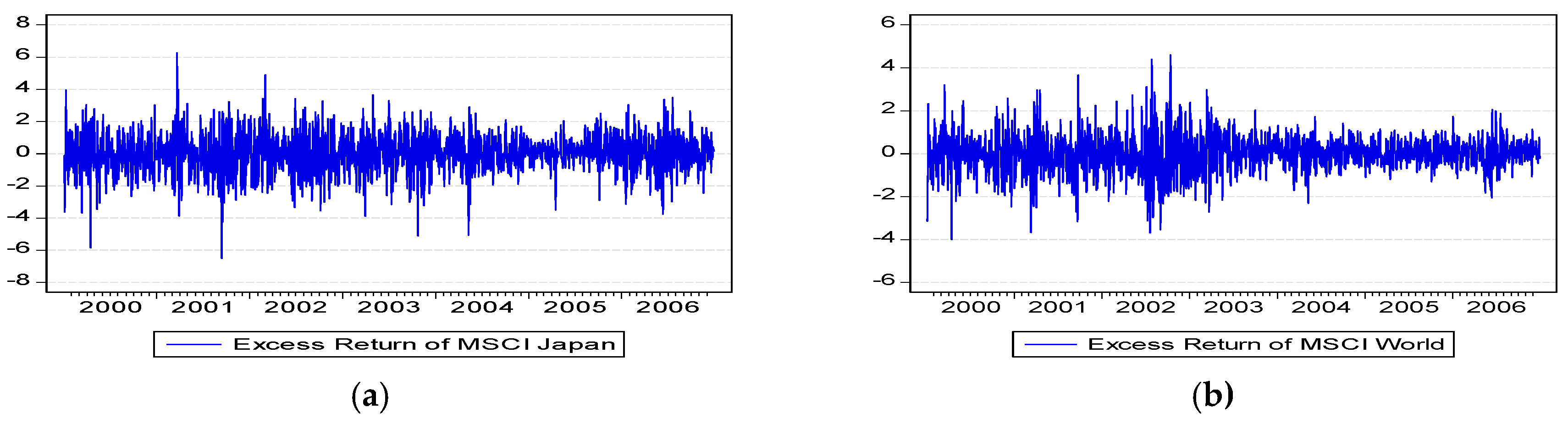
4.1. Japan Equity Funds

As it can be seen in Table 5, most of the Japan equity funds under the CPF Investment Scheme showed a negative volatility-timing coefficient, though the t-statistics were not significant in both single-index and three-index models without the currency risk effect. The t-statistics of Fund 4 showed significance for volatility-timing coefficient in a three-index model with no currency risk effect, which means that this fund was more aggressive than other funds in volatility timing. Their volatility-timing coefficients, (respectively; −0.155 and −0.173) also revealed that they respond more to abnormal market volatility. A negative coefficient suggested that a fund would get out of the market before volatility rises. When currency risk was included in the model specification, the other four CPF funds showed increasing response to the change of market conditional volatility by a more negative volatility-timing coefficient. Compared with the same model excluding currency risk effect, the t-statistics of most funds increased greatly in the models both with the currency risk effect and without it. Four out of the five funds under the CPF Investment Scheme had significant negative coefficients in the three-index models with the inclusion of currency risk, implying that these funds decreased their market exposure when market volatility was high. Such volatility reaction indicated active management of the funds and was likely to boot the expected portfolio return. This was because an actively managed fund should have a lower market beta simply because market volatility was low. Only one fund showed a positive volatility-timing coefficient in the single-index model, indicating that it lost money from volatility-timing as it did not reduce market exposure when market risk and volatility was high.
It can also be seen in Table 5 that for the non-CPF funds, there was only one fund with a significant negative coefficient for the volatility-timing in the three-index model when currency risk was excluded. Although the other three non-CPF funds had a negative coefficient in most cases, none were statistically significant. Similarly, there were three out of four funds showing an increasing response to the change of market conditional volatility with a greater negative coefficient when the currency risk was included.
Although the t-statistics of some individual funds were not significant, the average volatility timing coefficients for the CPF funds were found to be significant only when currency risk is included, though all are negative (Table 5). In contrast, the estimates were both negative and significant for the non-CPF funds with or without the currency risk included. In terms of magnitude, the latter was also larger than that for the CPF funds. As a volatile market is usually accompanied by negative market return, a lower negative volatility-timing coefficient implied that the CPF funds were more efficient in risk management which can in turn generate positive return in the volatile market. Furthermore, the average volatility-timing coefficient of CPF funds was found increased to −0.109 in the single-index model with currency risk, even lower than that for the non-CPF funds. This finding implies that currency risk plays an important role in the model specification of international asset management. This is consistent with our casual observation that the CPF Japan equity funds were more efficient in risk management.

4.2. Global Equity Fund

We report in Table 6 the volatility-timing estimates for the CPF and non-CPF global equity funds. As it can be seen, with the exception of Funds 5 and 6, the rest of the funds under CPF Investment Scheme showed a negative volatility-timing coefficient, though the t-statistics were not significant in both single-index and three-index models without currency effect. Both Funds 5 and 6 had a positive volatility-timing coefficient, implying that both funds become more exposed to market volatility and their investment strategy outweighed the volatile index stocks. Only Fund 4 showed a significant negative coefficient with a value being −0.172 and −0.181, respectively, in both the single-index model and three-index model without currency risk included, which revealed that the fund responds more to abnormal market volatility. When the model was corrected by including the currency risk effect, the volatility-timing coefficients of most funds became more negative. The negative volatility-timing coefficient with Funds 1, 3 and 7 became significant in both the single-index model and the three-index model. There were four out of seven CPF funds decreasing their exposure to the volatile market, which in turn, affected the return positively. Funds 5 and 6 remained with a positive volatility-timing coefficient in the model when the currency risk effect was included, implying that these funds lost money because of a decline in volatility timing.
The regression results about non-CPF global funds showed that, when the currency risk effect was excluded, only Fund 7 had a significant negative coefficient of volatility-timing in both the single-index and three-index models estimations. Fund 3 showed a significant positive volatility-timing coefficient at the 5% level. Although the other five non-CPF funds all had a negative volatility-timing coefficient, their t-statistics were not significant. Similar to the results of the non-CPF Japan equity fund, when the currency risk effect was considered, most funds showed an increasing response to the change of market conditional volatility with a decreasing negative volatility-timing coefficient, but the statistical significance level didn’t improve substantially.
The average volatility-timing coefficients of all CPF global equity fund were found to be non-significant, but all were significantly negative for the non-CPF fund in both the single-index and three-index models. This was largely due to the positive volatility-timing coefficients of two funds in the CPF group. Hence, it was inconclusive if the CPF global equity funds were more actively managing market risk and volatility based on the results of the group volatility-timing coefficients only.

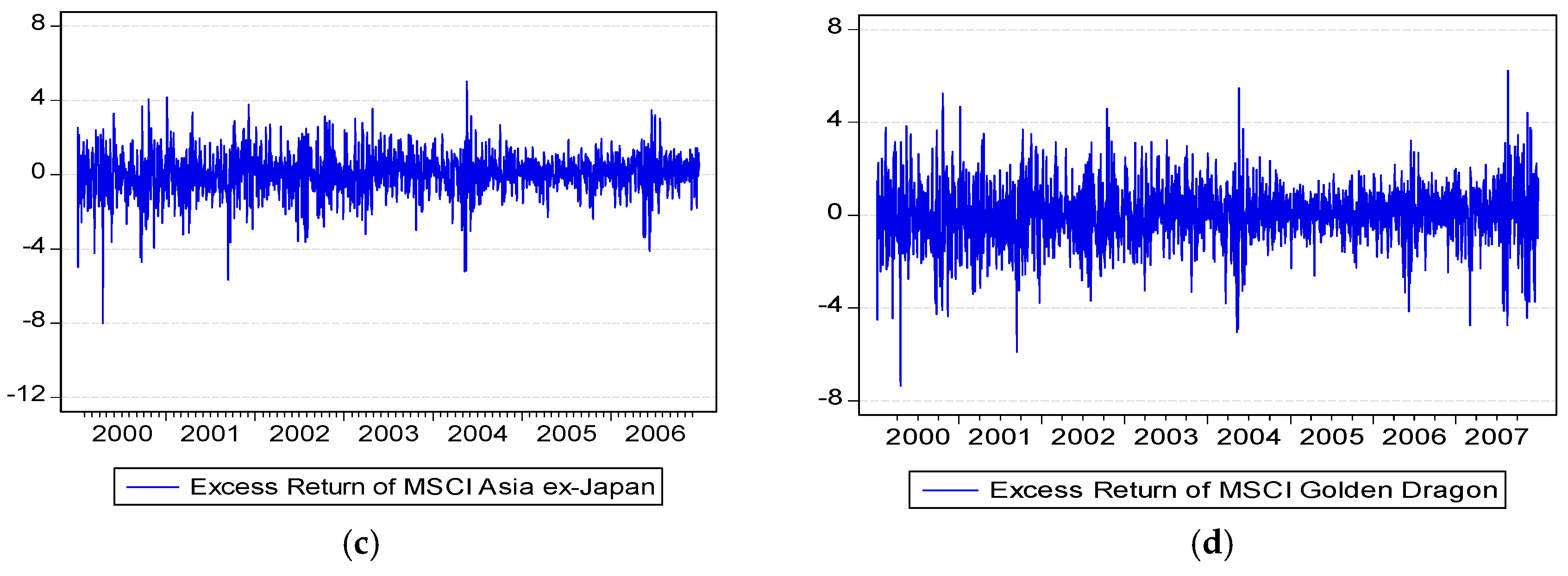
4.3. Asian Ex-Japan Equity Funds

The estimation results of the volatility-timing for the Asian ex-Japan funds under the CPF Investment Scheme and non-CPD funds are represented in Table 7.
As it can be seen in Table 7, most of the CPF funds showed a positive volatility-timing coefficient, though the t-statistics were not significant in both the single-index and the two-index models without currency risk. Fund 2 and Fund 3 showed negative volatility-timing coefficients in the two-index models with no currency effect, but were not statistically significant. Funds 1, 8, 9 and 10 all had a significant positive volatility-timing coefficient in both the single-index and the two-index models. The results suggest that these funds were bad performers in a turmoil market. A positive volatility-timing coefficient implied an increasing market exposure while the market became more volatile, which may contribute negatively to the funds’ return, given that market return was usually negatively correlated with volatility. The signs of volatility-timing coefficients and their t-statistics remained largely unchanged when currency risk was included in the model specification. When currency risk effect was considered, there were four funds out of 10 under the CPF Investment Scheme with significant positive estimates of volatility timing in the two-index models, which again suggested that these funds tended to increase their market exposure when market volatility was high and may have experienced a negative return.
The results of non-CPF Asian ex-Japan equity funds showed that, when the currency risk effect was excluded, only Fund 4 was found to have a negative coefficient though insignificant, and all the rest have positive estimates of volatility timing. With the inclusion of currency risk, the estimation results remained largely the same.
The average volatility-timing coefficients of both CPF and non-CPF Asian ex-Japan equity funds were all positive with similar values, and the only difference was their significance level. The results indicated that both CPF and non-CPF funds failed to demonstrate any advantages in volatility-timing, even though the CPF funds were slightly better than the non-CPF funds in risk management.

4.4. Greater China Equity Funds

We reported the estimation results of both CPF-scheme and non-CPF scheme Greater China equity funds in Table 8. One may see in Table 8 that three out of five CPF funds had a significant positive volatility-timing coefficient in both the single-index and two-index models when currency risk was not considered. Although Funds 2 and 3 both had a negative volatility-timing coefficient, they were statistically not significant. When the currency risk effect was included in the model specifications, these estimates barely changed, both in terms of magnitude and the significance level. Hence, the results seem to suggest that Greater China equity funds under CPF Investment Scheme are likely to increase their market exposure when market volatility is high. Such volatility reaction indicates passive management of market risk, and is likely to reduce the expected portfolio return as its market beta will be higher due to the high market volatility.
There were only two non-CPF Greater China equity funds available in Singapore. The results in Table 8 show that the estimates of volatility-timing in all models for Fund 1 were positive and statistically significant, but for Fund 2 all were negative and insignificant. When the currency risk effect was included, the results barely changed. This finding was very similar to that for the Greater China equity funds under the CPF Investment Scheme. Finally, the results showed that the average volatility-timing coefficients of both the CPF and non-CPF Greater China equity funds all were positive but insignificant. It is clear that the market behavior of these equity funds did not show any advantage in volatility timing. They did not reduce their market exposure when market volatility was high. Such volatility reaction indicated passive management and was likely to face an average return penalty. The possible explanation was the lack of diversification for regional funds in Asia.

5. Conclusions

In this study, we examined the volatility-timing performance of Singapore-based funds under the CPF Investment Scheme and non-CPF linked funds by taking into account the currency risk effect on internationally managed funds. We employed GARCH models and modified factor models to capture the response of funds to the market abnormal conditional volatility including the day of the week effect. The results show that volatility timing was one of the factors contributing to the excess return of funds. When the currency risk effect was considered, most of the Japanese equity funds and global equity funds showed an increasing response to the change of market conditional volatility with a decreasing negative volatility-timing coefficient. The finding implies that currency risk plays an important role in the model specification of international asset management, and is also consistent with our casual observation that CPF Japan (and global) equity funds are more efficient in risk management. However, funds’ volatility-timing seems to be country-specific. Most of the Japanese equity funds and global equity funds under the CPF Investment Scheme were found to have the ability of volatility timing, but the Asian equity funds and the Greater China funds failed to demonstrate any volatility-timing ability. Those funds may have increased market exposure when the market volatility was high, which in turn decreased their performance and reduced the expected portfolio return. Moreover, there was no evidence that funds under the CPF Investment Scheme showed a better group performance of volatility timing. These findings have important policy implication in managing the CPF Investment Scheme.

Author Contributions

X.S., A.K.T. and Z.Z. conceived the paper, X.S. analyzed the data; X.S., A.K.T. and Z.Z. wrote and finalized the manuscript. All authors read and approved the final manuscript.

Funding

The third author wishes to acknowledge the financial support from the Sumitomo Foundation.

Acknowledgments

An early version of the paper was presented at the 20th International Congress on Modelling and Simulation, Adelaide, Australia, 1–6 December 2013. The authors wish to thank Chia-Lin Chang, Michael McAleer, Alan Wong, conference participants, and two anonymous referees for their constructive comments and suggestions on an early version of this paper.

Conflicts of Interest

The authors declare no conflicts of interest.

References

  1. Busse, Jeffrey A. 1999. Volatility Timing in Mutual Funds: Evidence from Daily Returns. Review of Financial Studies 12: 1009–41. [Google Scholar] [CrossRef]
  2. Chen, Yong, and Bing Liang. 2007. Do market timing hedge funds time the market? Journal of Financial and Quantitative Analysis 42: 827–56. [Google Scholar] [CrossRef]
  3. Cooper, Tooper. 2010. Alpha Generation and Risk Smoothing Using Managed Volatility. Working Paper. Available online: http://ssrn.com/abstract=1664823 (accessed on 23 July 2019).
  4. Dubois, M., and P. Louvet. 1996. The day-of-the-week Effect: The International Evidence. Journal of Banking & Finance 20: 1463–84. [Google Scholar]
  5. Fama, Eugene F., and Kenneth R. French. 1993. Common Risk Factors in the Return on Stocks and Bonds. Journal of Financial Economics 33: 3–56. [Google Scholar] [CrossRef]
  6. Ferson, Wayne, and Haitao Mo. 2016. Performance measurement with selectivity, market and volatility timing. Journal of Financial Economics 121: 93–110. [Google Scholar] [CrossRef]
  7. Fleming, Jeff, Chris Kirby, and Barbara Ostdiek. 2001. The economic value of volatility timing. Journal of Finance 56: 329–52. [Google Scholar] [CrossRef]
  8. Fleming, Jeff, Chris Kirby, and Barbara Ostdiek. 2003. The economic value of volatility timing using “realized” volatility. Journal of Financial Economics 67: 473–509. [Google Scholar] [CrossRef]
  9. Giambona, Erasmo, and Joseph Golec. 2009. Mutual fund volatility timing and management fees. Journal of Banking & Finance 33: 589–99. [Google Scholar]
  10. Hallerbach, Winfried G. 2012. A proof of the optimality of volatility weighting over time. The Journal of Investment Strategies 1: 87–99. [Google Scholar] [CrossRef]
  11. Hallerbach, Winfried G. 2013. Advances in Portfolio Risk Control: Risk! Parity? Working Paper, Quantitative Strategies-Robeco Investment Management. Working Paper. Available online: http://ssrn.com/abstract=2259041 (accessed on 23 July 2019).
  12. Ho, Kin-Yip, YanLin Shi, and ZhaoYong Zhang. 2017. Does news matter in China’s foreign exchange market? Chinese RMB volatility and public information arrivals. International Review of Economics & Finance 52: 302–21. [Google Scholar]
  13. Ho, Kin-Yip, YanLin Shi, and ZhaoYong Zhang. 2018. Public information arrival, price discovery and dynamic correlations in the Chinese renminbi markets. The North American Journal of Economics and Finance 46: 168–86. [Google Scholar] [CrossRef]
  14. Jayasinghe, Prabhath, Albert K. Tsui, and ZhaoYong Zhang. 2014a. Exchange Rate Exposure of Sectoral Returns and Volatilities: Further evidence from Japanese industrial sectors. Pacific Economic Review 19: 216–36. [Google Scholar] [CrossRef]
  15. Jayasinghe, Prabhath, Albert K. Tsui, and ZhaoYong Zhang. 2014b. New Estimates of Time-Varying Currency Betas: A trivariate BEKK-GARCH approach. Economic Modelling 42: 128–39. [Google Scholar] [CrossRef]
  16. Jensen, Michael C. 1968. The Performance of Mutual Funds in the Period 1945–1964. Journal of Finance 23: 389–416. [Google Scholar] [CrossRef]
  17. Jensen, Michael C. 1969. Risk, the Pricing of Capital Assets, and the Evaluation of Investment Portfolios. Journal of Business 42: 167–247. [Google Scholar] [CrossRef]
  18. Jensen, Michael C. 1972. Optimal Utilization of Market Forecasts and the Evaluation of Investment Performance. In Mathematical Methods in Investment and Finance. Edited by G. P. Szego and Karl Shell. Amsterdam: Elsevier. [Google Scholar]
  19. Jiang, George J., Tong Yao, and Tong Yu. 2007. Do mutual funds time the market? Evidence from portfolio holdings. Journal of Financial Economics 86: 724–58. [Google Scholar] [CrossRef]
  20. Koh, Benedict S. K., Olivia S. Mitchell, Toto Tanuwidjaja, and Joelle Fong. 2007. Investment Patterns in Singapore’s Central Provident Fund System. Journal of Pension Economics and Finance 7: 37–65. [Google Scholar] [CrossRef]
  21. Lim, Guay C. 2005. Currency Risk in Excess Equity Returns: A Multi Time-varying Beta Approach. Journal of International Financial Markets, Institutions & Money 15: 189–207. [Google Scholar]
  22. Long, Ling, Albert K. Tsui, and Zhaoyong Zhang. 2014. Conditional Heteroscedasticity with Leverage Effect in Stock Returns: Evidence from the Chinese Stock Market. Economic Modelling 37: 89–102. [Google Scholar] [CrossRef]
  23. Marquering, Wessel, and Marno Verbeek. 2004. The economic value of predicting stock index returns and volatility. The Journal of Financial and Quantitative Analysis 39: 407–26. [Google Scholar] [CrossRef]
  24. Martinet, Guillaume Gaetan, and Michael McAleer. 2018. On The Invertibility of EGARCH (p, q). Econometric Reviews 37: 824–49. [Google Scholar] [CrossRef]
  25. McAleer, Michael. 2005. Automated inference and learning in modeling financial volatility. Econometric Theory 21: 232–61. [Google Scholar] [CrossRef]
  26. McAleer, Michael, and Marcelo C. Medeiros. 2008. A multiple regime smooth transition heterogeneous autoregressive model for long memory and asymmetries. Journal of Econometrics 147: 104–19. [Google Scholar] [CrossRef]
  27. Henriksson, Roy D., and Robert C. Merton. 1981. On Market Timing and Investment Performance II: Statistical Procedures for Evaluating Forecasting Skills. Journal of Business 54: 513–34. [Google Scholar] [CrossRef]
  28. Moreira, Alan, and Tyler Muir. 2017. Volatility-Managed Portfolios. The Journal of Finance 72: 507–27. [Google Scholar] [CrossRef]
  29. Moreira, Alan, and Tyler Muir. 2019. Should Long-Term Investors Time Volatility? Journal of Financial Economics 131: 507–27. [Google Scholar] [CrossRef]
  30. Nelson, Daniel B. 1991. Conditional heteroskedasticity in asset returns: A new approach. Econometrica: Journal of the Econometric Society 59: 347–70. [Google Scholar] [CrossRef]
  31. Qin, Fengming, Junru Zhang, and Zhaoyong Zhang. 2018. RMB Exchange Rates and Volatility Spillover across Financial Markets in China and Japan. Risks 6: 120. [Google Scholar] [CrossRef]
  32. Sharpe, W. F. 1966. Mutual Fund Performance. Journal of Business 39: 119–38. [Google Scholar] [CrossRef]
  33. Shen, Xiaoyi, Albert K. Tsui, and Zhaoyong Zhang. 2013. Modelling the Volatility-Timing of Funds under CPF Investment Scheme. Paper presented at the 20th International Congress on Modelling and Simulation, Adelaide, Australia, December 1–6; Available online: www.mssanz.org.au/modsim2013 (accessed on 23 July 2019).
  34. Sherman, Meadhbh, Niall O’Sullivan, and Jun Gao. 2017. The Market-Timing Ability of Chinese Equity Securities Investment Funds. International Journal of Financial Studies 5: 22. [Google Scholar] [CrossRef]
  35. Tang, Yi, and Robert F. Whitelaw. 2011. Time-Varying Sharpe Ratios and Market Timing. Quarterly Journal of Finance 1: 465–93. [Google Scholar] [CrossRef]
  36. Treynor, Jack L., and Kay K. Mazuy. 1966. Can Mutual Funds Outguess the Market? Harvard Business Review 44: 131–36. [Google Scholar]
  37. Yi, Li, Zilan Liu, Lei He, Zilong Qin, and Shunli Gan. 2018. Do Chinese mutual funds time the market? Pacific-Basin Finance Journal 47: 1–19. [Google Scholar] [CrossRef]
1
An earlier version of this paper with some preliminary findings was presented in the 20th International Congress on Modelling and Simulation (see Shen et al. 2013).
2
The CPF investment scheme was introduced in 1986 by the Singapore government in order to enhance CPF members’ funds for retirement. There are two accounts under the current CPF investment scheme, namely ordinary account (OA) and special account (SA). The instruments under CPF-SA are usually regarded to have higher risk than those under CPF-OA. CPF members can only invest in selected unit trusts, ETFs and investment-linked insurance products under the CPF-SA. The CPF board sets up strict admission criteria for investment products, especially for funds which tend to enter the CPF investment scheme. There are 28 fund management companies under the current CPF investment scheme, and 11 insurers under CPF Investment Scheme. Compared with the existing funds within the risk level under CPF Investment Scheme, new funds are required to have lower-than-median expense ratio. A good historical performance for at least three years is desirable. See also Koh et al. (2007).
Figure 1. Daily excess returns of markets: (a) MSCI Japan; (b) MSCI World; (c) MSCI Asian ex-Japan and (d) MSCI Golden Dragon.
Risks 07 00106 g001aRisks 07 00106 g001b
Table 1. Descriptive statistics of the excess returns of Japan equity funds under the Central Provident Fund (CPF) Investment Scheme and non-CPF Japan equity funds.
JPCPF1JPCPF2JPCPF3JPCPF4JPCPF5JPNCPF1JPNCPF1JPNCPF1JPNCPF1
Mean−0.017−0.008−0.025−0.016−0.002−0.018−0.0210.002−0.022
Median0.0000.0000.0000.0000.0000.0000.0000.0000.000
Max5.5615.8496.95217.4505.9995.9147.4345.8996.971
Min−5.615−6.234−6.233−18.834−8.976−9.106−9.682−6.418−8.073
Std. Dev.1.2161.3181.3941.5241.2871.2781.4221.1041.380
Skew.−0.072−0.012−0.071−0.428−0.415−0.382−0.570−0.131−0.298
Kurtosis4.5254.5265.28730.3657.0876.7186.8445.4656.364
DF-Test−43.065−40.866−40.149−45.356−37.650−36.005−37.435−41.343−38.054
Obs182418241824182418241824182418241824
Notes: JPCPF refers to Japan equity funds under the CPF Investment Scheme and JPNCPF refers to non-CPF funds. The number refers to the fund number. DF-test is the Dickey–Fuller Test. Obs stands for the number of observations.
Table 2. Descriptive statistics of the excess returns of global equity funds under the CPF Investment Scheme and non-CPF global equity funds.
(a) Global equity funds under CPF Investment Scheme
GlCPF1GlCPF2GlCPF3GlCPF4GlCPF5GlCPF6GlCPF7
Mean0.005−0.010−0.010−0.004−0.031−0.021−0.003
Median−0.004−0.006−0.0060.052−0.005−0.008−0.005
Max4.7755.5116.6126.8255.6036.9907.871
Min−5.809−5.995−6.913−6.913−6.834−5.641−9.924
Std. Dev.1.0470.9741.0991.0491.0851.0700.877
Skew.0.039−0.080−0.033−0.158−0.2180.207−0.861
Kurtosis5.4327.0326.2176.5986.6607.51419.373
DF-Test−38.696−40.405−38.795−39.884−37.258−42.548−38.743
Obs1824182418241824182418241824
(b) Non-CPF global equity funds
GNCPF1GNCPF2GNCPF3GNCPF4GNCPF5GNCPF6GNCPF7
Mean−0.023−0.032−0.0150.022−0.0120.013−0.009
Median−0.005−0.0050.0200.029−0.0060.029−0.006
Max4.84945.3284.8863.2595.8094.1823.665
Min−4.576−46.844−7.675−4.993−5.894−4.842−6.973
Std. Dev.0.9811.9141.1170.5911.0390.7680.866
Skew.−0.047−0.773−0.245−0.402−0.110−0.197−0.402
Kurtosis5.889370.2455.9318.9915.8736.2756.690
DF-Test−37.647−39.000−42.275−37.108−41.031−36.427−38.399
Obs1824182418241824182418241824
Notes: GlCPF refers to global equity funds under CPF Investment Scheme and GNCPF refers to non-CPF funds. The number refers to the fund number. DF-test is the Dickey–Fuller test. Obs stands for the number of observations.
Table 3. Descriptive statistics of the excess returns of Asian ex-Japan funds under the CPF Investment Scheme and non-CPF Asia ex-Japan funds.
(a) Asian ex-Japan equity funds under CPF Investment Scheme
ACPF1ACPF2ACPF3ACPF4ACPF5ACPF6ACPF7ACPF8ACPF9ACPF10
Mean0.0400.0060.0170.0150.0130.0210.0080.0170.0160.018
Median0.044−0.0060.010−0.007−0.002−0.006−0.006−0.007−0.007−0.006
Max3.5575.9214.8775.2847.4055.01710.9235.3845.3995.185
Min−6.549−13.636−7.552−10.546−8.666−9.021−12.44−8.755−8.087−9.008
Std. Dev.0.7881.1831.0311.2591.1421.0511.3101.0311.2271.181
Skew.−0.961−1.147−0.505−0.563−0.304−0.742−0.759−0.787−0.497−0.523
Kurtosis10.07116.7357.0077.5667.4048.06014.08710.1976.2587.323
DF-Test−38.247−36.379−37.137−39.742−39.84−39.62−41.52−39.82−39.08−38.79
Obs1824182418241824182418241824182418241824
(b) Asian ex-Japan equity funds under CPF Investment Scheme
ANCPF1ANCPF2ANCPF3ANCPF4
Mean0.0180.0040.0060.013
Median−0.007−0.006−0.006−0.006
Max6.4685.5286.3787.062
Min−12.579−10.419−9.111−8.462
Std. Dev.1.1761.3151.3271.232
Skew.−0.946−0.415−0.262−0.285
Kurtosis12.9007.1996.5326.698
DF-Test−39.934−41.203−37.223−38.189
Obs1824182418241824
Notes: ACPF refers to Asian ex-Japan equity funds under the CPF Investment Scheme and ANCPF refers to non-CPF funds. The number refers to the fund number. DF-test is the Dickey-Fuller test. Obs stands for the number of observations.
Table 4. Descriptive statistics of the excess returns of Greater China funds under the CPF Investment Scheme and non-CPF Greater China funds.
GCCPF1GCCPF2GCCPF3GCCPF4GCCPF5GCNCPF1GCNCPF2
Mean0.0420.0410.0370.0360.0230.0630.020
Median−0.005−0.003−0.006−0.0050.024−0.004−0.006
Max7.5234.1575.9616.2904.6688.6275.867
Min−8.383−8.729−9.765−10.466−9.952−8.482−9.549
Std. Dev.1.2631.0901.2711.3341.2201.4891.289
Skew.−0.362−0.580−0.355−0.538−0.836−0.327−0.409
Kurtosis7.0656.8536.9267.8209.0857.3036.733
DF-Test−41.684−43.071−41.284−41.611−41.247−24.186−42.026
Obs2085208520852085208520852085
Notes: GCCPF refers to Greater China funds equity funds under CPF Investment Scheme and GCNCPF refers to non-CPF funds. The number refers to the fund number. DF-test is the Dickey–Fuller Test. Obs stands for the number of observations.
Table 5. Volatility-timing coefficients for Japan equity funds under the CPF Investment Scheme and non-CPF funds.
CPF FundsNon-CPF Funds
FundsWithout Currency RiskWith Currency RiskWithout Currency RiskWith Currency Risk
Single-IndexThree-IndexSingle-IndexThree-IndexSingle-IndexThree-IndexSingle-IndexThree-Index
γ m p γ m p γ m p γ m p γ m p γ m p γ m p γ m p
Fund 1−0.041−0.048−0.074−0.082−0.048−0.080−0.099−0.134
(0.95)(1.10)(1.77)(1.96) *(0.83)(1.50)(1.79)(2.64) **
Fund 2−0.071−0.077−0.112−0.121−0.016−0.054−0.017−0.057
(1.54)(1.70)(2.57) *(2.78) **(0.41)(1.55)(0.44)(1.61)
Fund 30.0570.0390.010−0.011−0.032−0.040−0.031−0.040
(1.30)(0.90)(0.25)(0.27)(1.18)(1.49)(1.15)(1.48)
Fund 4−0.155−0.173−0.128−0.145−0.064−0.090−0.090−0.118
(2.29) *(2.55) *(1.91)(2.16) *(1.52)(2.19) *(2.17) *(2.93) **
Fund 5−0.060−0.085−0.106−0.133----
(1.17)(1.72)(2.16) *(2.84) **----
γ ¯ m p −0.155−0.173−0.109−0.121−0.040−0.090−0.090−0.126
Group t-value(1.592)(2.018)(3.331) *(4.053) *(3.87) *(5.730) **(2.872) *(3.814) *
Notes: As the volatility-timing coefficients for different funds were independent, the group t-statistic was calculated as, t = E ( γ i ) S T D ( γ ) n , where γ is the funds’ volatility-timing coefficients and n is the number of funds. The t-value is reported in parenthesis. *(**) Indicates significance at 5% and 1%, respectively.
Table 6. Volatility-timing coefficients for global equity funds under the CPF Investment Scheme and non-CPF funds.
CPF FundsNon-CPF Funds
FundsWithout Currency RiskWith Currency RiskWithout Currency RiskWith Currency Risk
Single-IndexThree-IndexSingle-IndexThree-IndexSingle-IndexThree-IndexSingle-IndexThree-Index
γ m p γ m p γ m p γ m p γ m p γ m p γ m p γ m p
Fund 1−0.047−0.020−0.093−0.0450.0300.0100.0190.010
(1.56)(0.64)(3.09) **(1.50)(1.30)(0.45)(0.84)(0.44)
Fund 2−0.060−0.019−0.067−0.0310.044−0.053−0.124−0.117
(0.89)(0.28)(0.98)(0.45)(0.33)(0.38)(0.91)(0.85)
Fund 3−0.024−0.058−0.115−0.0950.136−0.076−0.068−0.136
(0.49)(1.15)(2.36) *(1.92)(2.31) *(1.33)(1.25)(2.49) *
Fund 4−0.172−0.181−0.175−0.182−0.033−0.018−0.033−0.031
(3.33) **(3.40) **(3.32) **(3.40) **(1.53)(0.78)(1.53)(1.41)
Fund 50.2130.2250.1930.215−0.118−0.059−0.103−0.062
(3.69) **(3.77) **(3.28) **(3.60) **(1.69)(0.82)(1.45)(0.86)
Fund 60.2110.1130.1120.084−0.046−0.010−0.0020.003
(5.03) **(2.67) **(2.74) **(2.03) *(1.49)(0.31)(0.08)(0.08)
Fund 7−0.056−0.085−0.127−0.114−0.124−0.156−0.192−0.183
(1.37)(2.01) *(3.12) **(2.75) **(3.13) **(3.84) **(4.87) **(4.56) **
γ ¯ m p 0.084−0.0184−0.0342−0.0075−0.006−0.156−0.192−0.160
Group t-value(0.17)(0.071)(0.75)(0.48)(0.45)(2.48) **(2.57) **(2.65) **
Notes: As the volatility-timing coefficients for different funds were independent, the group t-statistic was calculated as, t = E ( γ i ) S T D ( γ ) n , where γ is the funds’ volatility-timing coefficients and n is the number of funds. The t-value is reported in parenthesis. *(**) Indicates significance at 5% and 1%, respectively.
Table 7. Volatility-timing coefficients for Asian ex-Japan equity funds under CPF Investment Scheme.
CPF FundsNon-CPF Funds
FundsWithout Currency RiskWith Currency RiskWithout Currency RiskWith Currency Risk
Single-IndexThree-IndexSingle-IndexThree-IndexSingle-IndexThree-IndexSingle-IndexThree-Index
γ m p γ m p γ m p γ m p γ m p γ m p γ m p γ m p
Fund 10.0820.080.0810.0790.1240.1240.1210.121
(3.16) **(3.14) **(3.14) **(3.12) **(2.65) **(2.64) **(2.62) **(2.61) **
Fund 2−0.06−0.058−0.061−0.0590.0850.0860.0840.086
(−1.26)(−1.22)(−1.29)(−1.26)(2.12) *(2.16) *(2.11) *(2.16) *
Fund 3−0.003−0.004−0.002−0.0030.0570.0580.0570.057
(−0.1)(−0.13)(−0.07)(−0.1)(1.69)(1.71)(1.68)(1.7)
Fund 40.0150.0170.0120.014−0.017−0.015−0.017−0.015
(0.38)(0.43)(0.31)(0.35)(0.62)(0.56)(0.62)(0.56)
Fund 50.020.0220.0170.018----
(0.68)(0.73)(0.6)(0.64)----
Fund 60.10.0990.0990.098----
(2.64) **(2.61) **(2.62) **(2.60) **----
Fund 70.0350.0370.0330.035----
(0.89)(0.94)(0.85)(0.9)----
Fund 80.1180.1180.1160.116----
(2.65) **(2.65) **(2.63) **(2.62) **----
Fund 90.0590.0610.0580.06----
(1.43)(1.49)(1.4)(1.46)----
Fund 100.1020.1020.0980.099----
(3.54) **(3.57) **(3.57) **(3.59) **----
γ ¯ m p 0.1010.09980.09850.0980.1050.1050.1050.104
Group t-value2.65 **2.72 **2.57 **2.64 **2.092.15*2.102.16 *
Notes: As the volatility-timing coefficients for different funds were independent, the group t-statistic was calculated as, t = E ( γ i ) S T D ( γ ) n , where γ is the funds’ volatility-timing coefficients and n is the number of funds. The t-value is reported in parenthesis. *(**) Indicates significance at 5% and 1%, respectively.
Table 8. Volatility-timing coefficients for Greater China equity funds under CPF Investment Scheme and non-CPF funds.
CPF FundsNon-CPF Funds
FundsWithout Currency RiskWith Currency RiskWithout Currency RiskWith Currency Risk
Single-IndexThree-IndexSingle-IndexThree-IndexSingle-IndexThree-IndexSingle-IndexThree-Index
γ m p γ m p γ m p γ m p γ m p γ m p γ m p γ m p
Fund 10.1090.1060.110.1070.1790.1810.1790.180
(3.37) **(3.28) **(3.41) **(3.32) **(3.22) **(3.25) **(3.22) **(3.25) **
Fund 2−0.055−0.051−0.054−0.05−0.022−0.024−0.02−0.021
−1.74−1.64−1.71−1.6(0.72)(0.75)(0.66)(0.68)
Fund 3−0.024−0.021−0.026−0.023----
(0.77(0.68)(0.87)(0.78)----
Fund 40.1460.1420.1480.145----
(4.91) **(4.81) **(5.17) **(5.09) **----
Fund 50.1190.1160.1190.116----
(4.09) **(4.00) **(4.08) **(3.99) **----
γ ¯ m p 0.06860.06680.06980.06820.1790.1810.1790.180
Group t-value(1.85)(1.87)(1.89)(1.90)(0.78)(0.77)(0.80)(0.79)
Notes: As the volatility-timing coefficients for different funds were independent, the group t-statistic was calculated as, t = E ( γ i ) S T D ( γ ) n , where γ is the funds’ volatility-timing coefficients and n is the number of funds. The t-value is reported in parenthesis. *(**) Indicates significance at 5% and 1%, respectively.

