Estimating Territory Risk Relativity Using Generalized Linear Mixed Models and Fuzzy C-Means Clustering ^†

Abstract

Territory risk analysis has played an important role in auto insurance rate regulation. It aims to design rating territories from a set of basic rating units so that their respective risk relativities can be estimated to reflect the regional risk of insurance. In this work, spatially constrained clustering is first applied to insurance loss data to form such regions, using the forward sortation area (FSA) as a basic rating unit. The groupings of FSA by spatially constrained clustering reduce the insurance rate heterogeneity caused by smaller risk exposures. Furthermore, the generalized linear mixed model (GLMM) is proposed to derive the risk relativities of clusters and each FSA. In addition, as an alternative approach, fuzzy C-Means clustering is proposed to derive the risk relativity of FSA, and the obtained results are compared to the ones from GLMM. The spatially constrained clustering and risk relativity estimation help to retrieve a set of territory risk benchmarks used in rate filings within the regulation process. It also provides guidance for auto insurance companies on rate making.

1. Introduction

In the territory risk analysis of auto insurance, the residential information such as postal codes or zip codes is used as a basic pricing unit Yao (2008). The type of geographical data used for territorial risk depends on the country. For example, in the USA, the loss data associated with zip codes are often used for insurance pricing (Halder et al. 2021; Nasseh et al. 2021). This work studies the geographical loss data based on FSA, the first three characters of Canadian postal codes. The main reason for using FSA instead of postal codes is that each FSA contains more risk exposures than an area covered by a single postal code. This approach can better reflect the actual loss pattern and stabilize the risk relativities to minimize the fluctuations among the calculations using data from different accident years or data-reporting years. However, determining risk relativity based on FSA as the only source may not be sufficient to reflect the territory risk. To further study other sources that impact the risk relativity of FSA, we consider the effect of the city as a variable, since postal codes or zip codes are nested within a city or town. These potential effects on insurance loss patterns may be, in fact, due to some factors associated with the city or town. For instance, people tend to drive more in a city where commuter buses or public transportation are relatively limited. Because of the high level of vehicle usage, the likelihood of causing a car accident could be higher than when the usage of vehicles is low. This high usage of vehicles may potentially increase the loss cost of auto insurance and the expenses required to settle insurance claims Ma et al. (2018). Therefore, the risk relativities in these areas should be higher than in others. A recent study Litman (2018) shows that annual crash rates and insurance claim costs tend to increase with annual vehicle travel. This may explain why Usage-Based Insurance (UBI) is an emerging pricing strategy in auto insurance, and it has become a major research area in insurance data science (Blais et al. 2020; Fang et al. 2021; Stankevich et al. 2022).

This paper is an extended version of the conference paper that appeared in Xie et al. (2021). In Xie et al. (2021), a method using generalized linear mixed models (GLMM) was proposed to derive the risk relativities for a set of clusters. These clusters were produced by spatially constrained clustering, where spatial continuity was considered Xie (2019). GLMM are an extension of generalized linear models (GLM) (David 2015; Goldburd et al. 2016; Kafkova and Křivánková 2014), in which the model contains both fixed and random effects (Dean and Nielsen 2007; Jiang and Nguyen 2007; Stroup 2012). The risk relativities for FSAs were obtained using GLMM, which involves the multilevel modeling of geographical loss costs. Within this multilevel modeling approach, the impact of differences among cities or towns can be captured, and the model better reflects the risk relativity associated with different cities. Using the root mean square error (RMSE) and mean average deviation (MAD), we measured the smoothing errors using results obtained from GLMM and the empirical geographical risk relativities. We assumed that the risk relativity of FSA is at the cluster level, which means that FSA risk relativities are the same for all FSA within the same cluster. The results presented in Xie et al. (2021) are preliminary, and further investigation within the approach and a comparison to other related techniques are essential to help us to better understand the impact of the proposed method on auto insurance rate regulation.

In spatially constrained clustering Xie (2019), each FSA is classified into one cluster, and GLMM is used to estimate the risk relativity of each cluster further, so as to remove data noise to achieve a smoothing effect on the empirical estimate of FSA risk relativity. Achieving a smoothing result implies that we focus on the major data pattern. In this approach, the geographical risk relativity is the same for each FSA that belongs to the same cluster. In this revised and extended version, we shift our focus on the estimation of geographical risk relativity from a hard approach to a soft method. We propose to use fuzzy C-Means clustering (Ansari and Riasi 2016; Yan et al. 2021; Yeo et al. 2003) to obtain a fuzzy number for each FSA. Fuzzy C-Means clustering is not necessarily novel in insurance pricing, as it is a commonly used technique in data analysis and machine learning. The fuzzy C-Means clustering method has also been successfully used in risk analysis. For example, in Jafarzadeh et al. (2017), fuzzy C-Means clustering was used to estimate the forest fire risk. The data were also assumed to belong to clusters with different degrees of membership. In De Andres et al. (2011), fuzzy C-Means clustering was combined with multivariate adaptive regression splines to forecast bankruptcy. Their results showed that the approach outperformed the other methods’ classification accuracy and the profit generated by lending decisions. However, it is particularly novel and valuable in insurance rate regulation because of the complexity of insurance loss data and the need for more meaningful and targeted risk assessments at the industry level, such as territory design.

In K-Means clustering (Bhowmik 2011; Nian et al. 2016; Thakur and Sing 2013), each data point is assigned to only one cluster based on the distance between the observation and the cluster centroid. However, fuzzy C-Means clustering allows for more flexible cluster assignments by assigning each data point a membership value for each cluster. This membership value indicates the degree to which the observation belongs to each group, rather than a binary assignment to a single cluster. Thus, each FSA will belong to all clusters that we design with different membership coefficients. Our objective of using fuzzy C-Means is to move from the multilevel model to a fuzzy approach that allows each FSA to be influenced by all possible neighboring FSA, rather than only the city to which the FSA belongs. It is an unsupervised machine learning technique, which we have applied in a novel way to actuarial science.

One of the current challenges in using machine learning for auto insurance rate regulation is ensuring that the algorithms used are transparent and explainable (Dhieb et al. 2019; Hanafy and Ming 2021; Pranavi et al. 2020). This is particularly important because many regulators require insurers to explain their modeling tools and pricing decisions. Both GLMM and fuzzy clustering meet this need, and our method aims to provide more interpretable results on how the territory can be designed and how the associated relativities can be further estimated. Black box machine learning algorithms, which are difficult to interpret and explain, may lead to concerns regarding fairness and bias and may not be compliant with regulatory requirements. Therefore, insurers need to develop interpretable, transparent machine learning algorithms that can be easily explained to regulators and policyholders. Our method may serve as a guideline in solving territory design problems, which most auto insurance companies face regarding regulation rules.

Overall, this research aims to extend the current focus on territory risk analysis using hard clustering to a soft one. It also aims to further estimate the relativity estimate using a mixed model, rather than the traditional approach that uses generalized linear models. The proposed methods are considered a modern approach that may play an important role in the rate and classification of auto insurance regulation. In addition, it may be necessary to consider how to digitalize the spatial location in territory design, and different countries may face different levels of such difficulties in geocoding. Fuzzy clustering that makes use of all geocoded loss costs is a soft clustering approach. Unlike traditional hard clustering or spatially constrained clustering, it does not require us to address the cluster boundary or contiguity constraint on the territory design. Moreover, the mixed model, which introduces additional effects, further addresses the potential impact caused by different cities due to the different infrastructures and availability of local transportation systems. Therefore, it provides an alternative approach to analyzing territory risk for auto insurance. The proposed method also aims at guiding applications of soft clustering along with mixed models to analyze complex economic and financial data so that such more advanced statistical and computational methods can be promoted, in order to improve the novelty of research studies in the sense of having a new approach to solving real-world problems. Therefore, the proposed soft clustering method could become an alternative approach for territory design in auto insurance rate regulation.

The rest of this paper is organized as follows. In Section 3, the data and their processing are briefly introduced, and the proposed generalized linear mixed models, fuzzy C-Means clustering and the method to obtain the FSA risk relativities are discussed. In Section 4, the main results are summarized. Finally, we conclude our findings and provide further remarks in Section 5.

2. Related Work

In auto insurance rate making, territory risk and classification are crucial in the rate regulation process. Studying territorial risk and the relativity associated with each territory requires considerable effort. Because of this, a large amount of the work in territory analysis in auto insurance has been conducted. In Brubaker (1996), a geographic rate-making procedure was developed to estimate the risk relativity for any point on the map. The benefit of producing a surface as a map of loss data is that it does not require clustering or territory design. The work in Brubaker (1996) uses geo-coded loss data similar to ours. The difference is that we focus on the forward sortation area (FSA), while the work conducted in Brubaker (1996) is based on zip code data. In Xie (2019), spatially constrained clustering with an entropy method was proposed to determine the optimal number of clusters. The work in Xie (2019) addresses a fundamental problem in the rate and classification of auto insurance regulation: choosing the appropriate number of groups for the rate regulation purpose. However, it did not estimate the risk relativity for the clusters designed using spatially constrained clustering. In Jennings (2008), K-Means and other clustering techniques were used to define geographical rating territories for pricing purposes. However, the study does not address the spatial contiguity issue Grubesic (2008), one of the critical regulation rules. Furthermore, the estimation problem of the risk relativity associated with clusters obtained from clustering was not studied. Our work has focused on clustering problems and estimating the risk relativities of the basic rating unit, FSA.

Fuzzy C-Means clustering, an important soft computing approach, is now widely used in insurance, especially for fraud detection. In Majhi (2021), fuzzy clustering was used to optimize the cluster centroids and remove the outliers in an automobile insurance fraud detection system. The proposed method, along with a modified whale optimization algorithm, improved the detection accuracy using machine learning techniques as classification methods. Similarly, in Yan et al. (2021), simulated annealing genetic fuzzy C-Means clustering was used to obtain fuzzy association rules to identify fraud claims. In a two-stage insurance fraud claim detection system Subudhi and Panigrahi (2020), fuzzy C-Means clustering was used to identify the claim as genuine, malicious, or suspicious in the first analysis stage. Again, fuzzy clustering helped to eliminate the outliers among sample data. The fuzzy clustering approach is not only successfully applied in insurance but also in financial auditing. For instance, in Aktas and Cebi (2022), the authors found that, using fuzzy C-Means, a success rate of 92% could be achieved in detecting fraudulent financial transactions. The ability to detect irregularities in financial auditing significantly improves the review and auditing efficiency.

GLMM has been successfully utilized in actuarial science as a rate-making technique Jeong et al. (2017) and a model for credibility to deal with repeated measurements or longitudinal data Antonio and Beirlant (2007). In Sun and Lu (2022), a Bayesian generalized linear mixed model was proposed for data breach incidents. The model sought to establish the relationship between the frequency and severity of cyber losses and the behavior of cyber attacks. The study in Sun and Lu (2022) shows the feasibility and effectiveness of using the proposed NB-GLMM to analyze the number of data breach incidents. In Yau et al. (2003), GLMM was used to model repeated insurance claim frequency data. Incorporating a conditionally fixed random effect into the model was considered an advantage as it provided a viable alternative in revising rates in general insurance. Our work applies GLMM in a novel way to estimate regional risk relativities. It is considered an extension of the approach that appeared in Xie and Lawniczak (2018) by further addressing the impact of other correlated factors on the territorial risk relativity estimates.

3. Materials and Methods

3.1. Data

We use a real dataset, part of the Automobile Statistical Plan data published by the Canadian General Insurance Statistical Agency. The Automobile Statistical Plan is a crucial source of complex high-dimensional data for auto insurance rate regulation Regan et al. (2008). In addition, there is an ongoing data collection, data reporting and data management process that provides a source of support for auto insurance rate making and rate regulation for both the industry and the government. The dataset used in this work includes the reported loss information from all auto insurance companies within a province for accident years 2009 to 2011. It consists of geographical loss information, including postal codes, cities, reported loss costs and earned exposures. The reported loss cost is the projected ultimate expected loss. This means that the loss cost has been considered for future loss development. The earned exposures refer to the total number of insured vehicles within a policy year. We first retrieved all postal codes associated with the same forward sortation area (FSA) level, where the FSA is recorded as the first three characters of the postal code. Then, for each FSA, the postal codes were further geo-coded using a geo-coder. The obtained geo-coding contains both average latitude and longitude values to represent the center of a given FSA. The centroid of the FSA is used to identify the location of the given FSA.

Due to the use of industry-level projected loss cost data, territory design is not conducted regularly in rate regulation. Unlike other benchmark values, the obtained results on territory design often continue to be used for an extended period until a periodic review of such results is initiated. Because of this, we continue using 2009 to 2011 FSA loss data for this investigation. This also allows us to make a meaningful comparison to the previous study on the same dataset with different approaches, such as the work in Xie (2019). On the other hand, we use loss cost data instead of claim frequency and severity data. This is because our investigation focuses on a regulation perspective. Often, the clustering results based on claim frequency differ from those under claim severity. Therefore, reconciling two sets of results by multiplying the respective risk relativity for each FSA may develop unnecessary uncertainty. From a theoretical point of review, under certain model assumptions, two sets of results (loss cost and splitting by claim frequency and severity) will lead to the same estimate of relativity for each FSA if no further clustering is involved. However, our proposed method aims to re-estimate the FSA relativity after obtaining the clusters. Therefore, it is more suitable and practically feasible if the loss cost is used.

We aim to estimate each cluster’s risk relativity so that the relativity of FSA can be further obtained. At a given level, the relativity of a risk factor is the risk level relative to the overall average for all risk levels that we consider. In this work, the loss cost at a given level is divided by the loss cost across all levels of territorial risk to calculate the risk relativity. Here, we consider the problem of estimating territory risk using a GLMM and the fuzzy C-Means clustering approach. For the GLMM method, we first need to cluster our spatial loss cost data into different clusters; then, we must apply GLMM to investigate the relationship between the loss cost and clusters and associations within different cities; lastly, we must estimate the risk relativity for each cluster. The risk relativity is assumed to be the same for FSA with the same cluster. Next, we aim to obtain a membership coefficient matrix for fuzzy C-Means clustering, which indicates the association between the FSA and cluster. Finally, we use this data matrix to further derive the risk relativity for each FSA.

3.2. Spatially Constrained K-Means Clustering

In this section, we briefly describe the spatially constrained K-Means clustering that was originally proposed in Xie (2019). The spatial constraint on the clustering is due to the regulation rule of being spatially contiguous for the designed territories. We apply this clustering algorithm to produce a set of clusters for our spatial loss cost data.

Let us assume that we have a d-dimensional real vector X, i.e., $X\in R^d$, with a set of observations {$X_1$, $X_2$, …, $X_n$}. In this work, $X_i$ represents the loss cost data associated with the ith FSA. K-Means clustering aims at partitioning these n observations into K sets ($K\le n$), S = $\{S_1,S_2,\dots ,S_K\}$, where $X_j$ belongs to one of the clusters, $S_i$, so that we can solve the following within-cluster sum of squares (WCSS) minimization problem, i.e.,

$$\begin{array}{c}\hfill arg\underset{S}{min}\sum _{i=1}^K\sum _{X_j\in S_i}{\parallel X_j-{\mathit{\mu }}_i\parallel }^2,\end{array}$$

(1)

where ${\mathit{\mu }}_i$ is the mean point of cluster $S_i$. We group the FSA loss cost data into K clusters by minimizing their WCSS. The input data for the K-Means clustering comprise a three-dimensional vector consisting of the normalized loss cost, normalized latitude and normalized longitude. In order to satisfy the requirement of spatial contiguity in rate regulation, we have to incorporate the spatial contiguity constraint, where the process of constructing a Delaunay Triangulation (DT) is involved. To better illustrate how a DT is constructed, we briefly describe the procedure as follows. For a more detailed description, we refer the reader to Xie (2019).

• A standard K-Means clustering was conducted, as an initial clustering, so that a set of clusters could be obtained.
• Based on the results obtained from the previous step, we searched all points that were entirely surrounded by points from other clusters. These points were denoted by non-contiguous points.
• The neighboring point at a minimal distance to the point that had no neighbors in the same cluster was found by performing a search.
• The points that had no neighbors were then reallocated to new clusters, and this process was continued until all clusters were formed into Delaunay Triangulations.

We assume an initial value in the first step of implementing K-Means clustering. The clustering results may depend on the choice of the number of clusters. In this work, for illustration purposes, the number of clusters used for clustering may not be the optimal choice of clusters, as we can use data visualization when the number of clusters is small. The selection of the optimal number of clusters has been fully addressed in Xie (2019) using an entropy-based approach. This work is considered a follow-up study after the clustering of spatial loss cost data. The aim is to determine each FSA’s risk relativity using GLM, GLMM and the fuzzy C-Means clustering-based approach.

3.3. Generalized Linear and Generalized Linear Mixed Models

Generalized linear models (GLM), as a flexible and interpretable model, can be used to handle a wide range of data types and distributions, including binary, count and continuous data. GLM are also computationally efficient and can handle large datasets. In rate making, GLM are often utilized because an exponential family distribution is a better choice in modeling the error function. GLM are widely used for territory risk analysis by transforming the expected loss cost values so that the predictors have a linear relationship with the transformed loss cost values. The loss cost, defined as the average loss per vehicle for a specified basic rating unit in territory risk analysis, serves as the response variable. In this study, we propose to extend the GLM to GLMM Antonio and Beirlant (2007) to account for the random effects of another rating variable. As an extension of GLM, GLMM retain the strengths of GLM, being flexible and interpretable, but they can be further used to handle correlated data by incorporating random effects that capture the correlation structure among the data.

The city infrastructure and public transportation influence driver behavior and accident occurrence. The availability of public transit in a city strongly affects how much drivers rely on their vehicles. To explain the GLMM, we assume that the loss cost data have been spatially grouped into K clusters, with a total of M different cities associated with the insurance loss cost data. Thus, the loss cost associated with cluster i and city j is defined as $L_{ij}$, where $i=1,2,\dots ,K$ and $j=1,2,\dots ,M$. We further define the expected value of the loss cost as ${\mu }_{ij}=E\left(L_{ij}\right)$. This expected value is then transformed by a given function $g(·)$ and defined as ${\eta }_i=g\left({\mu }_{ij}\right)$. The transformation function, referred to as the link function, is used to link the expected loss cost with the predictors.

The transformation function $g(·)$ is modeled using a linear mixed effect model, which includes both fixed and random effects and can be expressed as

$$\begin{array}{c}\hfill g\left({\mu }_{ij}\right)={\beta }_0+{\beta }_{1i}{x}_i+v_j,\end{array}$$

(2)

where $x_i$ represents the fixed effect of the ith cluster, and $v_j$ represents the random effect of the jth city.

In the generalized linear model, the variance of the model residual ${ϵ}_{ij}$ is assumed to have a functional relationship with the mean response, given by

$$\begin{array}{c}\hfill Var\left({ϵ}_{ij}\right)=\frac{\varphi V\left({\mu }_{ij}\right)}{{\omega }_{ij}},\end{array}$$

(3)

where $V\left(x\right)$ is the variance function, which is a result of the exponential family distribution. The parameter $\varphi$ scales the variance function $V\left(x\right)$, and ${\omega }_{ij}$ is a constant weight. Various distributions are used in this study, such as the normal distribution when $V\left(x\right)=1$, the Poisson distribution when $V\left(x\right)=x$, the gamma distribution when $V\left(x\right)=x^2$ and the inverse Gaussian distribution when $V\left(x\right)=x^3$. These distributions are special cases of the Tweedie distribution, commonly used in the actuarial field. Focusing on these special cases is sufficient for regulation as they are common in actuarial practice and easier to understand in guiding rate filings’ decision making. In $V\left(x\right)=x^p$, another parameter value of p is possible but may reduce the interpretability of the model because not every p has a distribution that one can refer to. To estimate the fixed and random effects, we use the glmer function available in the lme4 R package.

To derive the risk relativities for each FSA, we first determine the relativity of the fixed effect of the ith cluster, which is exp$\{{\widehat{\beta }}_{1i}\}$. The exponential transformation of the model coefficient is due to the log link function used in the GLMM. The estimate of the random effect $v_j$ is the conditional mode, which is the difference between the average predicted response for a given set of fixed effect values and the response predicted for a particular individual. Technically, these are the solutions to a penalized weighted least-squares estimation problem. We can consider these as individual-level effects, i.e., how much any individual loss cost differs from the population level due to the jth city. Because of this, the relativity corresponding to the jth city becomes $exp\{{\widehat{v}}_j\}$.

Therefore, the combined risk relativities due to fixed and random effects are calculated by $exp\{{\widehat{\beta }}_{1i}+\widehat{v}j\}$, and further divided by the average value of $exp\{{\widehat{\beta }}_{1i}+{\widehat{v}}_j\}$ for normalization. This normalization ensures that the expected value of the risk relativity is equal to 1. The risk relativities obtained in this way provide a measure of how the risk in a given FSA compares to the risk in the overall population after adjusting for the effects of clustering and the city-specific factors.

GLM assume that the data are independent and identically distributed, which may not be true when dealing with correlated data. This is why we propose to use GLMM instead. However, GLMM can be more complex to interpret than GLM due to the incorporation of random effects. In practice, GLMM can be difficult to fit and require careful consideration of the appropriate random effect structure. Moreover, a special software package is needed for the implementation of GLMM.

3.4. Estimating Risk Relativity via Fuzzy C-Means Clustering

In the previous section, we discussed a hard clustering approach using K-Means. We first obtain a set of clusters and use both GLM and GLMM to determine the risk relativity for each cluster. Using GLM, we impose that each FSA within the cluster has the same relativity. In contrast, the approach using GLMM allows us to modify the risk relativity of FSA further using a multi-level approach by incorporating the risk relativity of the city. We further consider a soft clustering approach via fuzzy C-Means clustering. The rationale is that car accidents often happen outside the driver’s residential area or even outside the city that the driver lives in. Theoretically, losses can occur anywhere. Thus, it is intuitively logical to carry out relativity calculations for FSA to take loss information from other cities (or other FSA). Moreover, the longer the distance from the residential area, the lower the probability of accident occurrence. This may be controlled by the membership coefficients obtained from the fuzzy C-Means clustering. Because of this, we propose to calculate the risk relativity of FSA based on fuzzy C-Means. In this case, fuzzy clustering allows FSA to belong to multiple clusters, which is useful when there is ambiguity or uncertainty in determining the group membership of loss data. In addition, since fuzzy clustering allows us to account for overlaps between clusters, it provides a more accurate representation of the underlying structure of FSA data. Because of this, it is unnecessary to further consider the continuity of the designed clusters and the boundary issue, which is an ongoing challenge in rate regulation practice.

For a d-dimensional real vector, i.e., $X_i\in R^d$, with a set of realizations {$X_1$, $X_2$, …, $X_n$}, the K-Means clustering in (1) can be reformulated as

$$\begin{array}{c}\hfill {arg}_{w,\mathit{\mu }}min\sum _{i=1}^K\sum _{j=1}^n{w}_{ij}{\parallel X_j-{\mathit{\mu }}_i\parallel }^2,\end{array}$$

(4)

with a matrix $W=\left(w_{ij}\right)$ of binary indicators such that $w_{ij}=1$ if $X_j$ is in the cluster that has centroid ${\mathit{\mu }}_i$; otherwise, it becomes zero if $X_j$ is in the cluster of centroid ${\mathit{\mu }}_i$. Fuzzy C-Means clustering aims at the partitioning of these n observations into a collection of C fuzzy clusters ($C\le n$) so that the weighted within-cluster sum of squares, which is given as follows, is minimized:

$$\begin{array}{c}\hfill \sum _{i=1}^C\sum _{j=1}^n{w}_{ij}\left(m\right){\parallel X_j-{\mathit{c}}_i\parallel }^2,\end{array}$$

(5)

where ${\mathit{c}}_i$ is the mean point of cluster $C_i$. The weight value, which is a function of m, is defined as

$$\begin{array}{c}\hfill w_{ij}\left(m\right)={\left(\sum _{k=1}^c{\left(\frac{\parallel X_j-{\mathit{c}}_i\parallel }{\parallel X_j-{\mathit{c}}_k\parallel }\right)}^{\frac{2}{m-1}}\right)}^{-m},\end{array}$$

(6)

where the center of the kth fuzzy cluster is denoted by

$$\begin{array}{c}\hfill {\mathit{c}}_k=\frac{{\sum }_{j=1}^n{w}_{kj}\left(m\right)X_j}{{\sum }_{j=1}^n{w}_{kj}\left(m\right)},\mathrm{for}k=1,2,\dots ,C.\end{array}$$

(7)

Here, the exponential weight, m, is the fuzziness that controls how likely it is that each observation will belong to each cluster.

To calculate the risk relativity of FSA, let $e_i$ denote the risk exposure for the ith FSA, and let $L_i$ denote the loss costs for the ith FSA. We can obtain the membership coefficient (denoted by $w_{ik}$), a fuzzy number to indicate how the ith FSA is related to a kth cluster, via the fuzzy C-Means clustering introduced above. We then use the risk exposures and loss costs to define the weighted loss costs (i.e., $l_{ik}$) for the ith FSA in the kth cluster as follows:

$$l_{ik}=\frac{w_{ik}{e}_i{L}_i}{{\sum }_{i=1}^N{w}_{ik}{e}_i}.$$

(8)

Furthermore, the weight value (${\alpha }_k$) applied to the kth cluster can be formulated as follows:

$${\alpha }_k=\frac{{\sum }_{i=1}^N{l}_{ik}}{\frac{1}{k}{\sum }_{k=1}^K{\sum }_{i=1}^N{l}_{ik}}.$$

(9)

Therefore, the risk relativity ($r_i$) for the ith FSA can be defined as the normalized average of the sum of the risk relativities among K clusters for the ith FSA, which is given as follows:

$$r_i=\frac{{\sum }_{k=1}^K{\alpha }_k{w}_{ik}}{\frac{1}{N}{\sum }_{i=1}^N{\sum }_{k=1}^K{\alpha }_k{w}_{ik}}.$$

(10)

An entropy-based approach was proposed to select the optimal number of clusters in spatially constrained clustering Xie (2019), which we presented in the previous study. The selection of the number of designed clusters was based on minimizing a regularized entropy measure. To select the number of fuzzy clusters, we use the smoothing errors calculated by MAD and RMSE. The suitable number of fuzzy clusters is then determined by the K that leads to a small MAD and RMSE. This article will explore the pattern of estimated relativities from our proposed methods, and the results will be presented and analyzed in the Results section.

3.5. Discussion

The approach of using fuzzy C-Means clustering and generalized linear mixed models to estimate risk relativity in auto insurance is a novel and promising method that combines the advantages of both techniques. Fuzzy C-Means clustering is a clustering technique that allows for overlapping clusters and considers the degree of membership of each entity to each cluster. This enables fuzzy C-Means clustering to capture the potential heterogeneity within groups and estimate the risk relativity more accurately. GLMM are widely used in insurance pricing due to their ability to simultaneously model individual-level territory risks and cluster-level effects. However, GLMM are limited in their ability to account for potential heterogeneity within clusters, leading to biased risk relativity estimates.

Auto insurance risk factors vary greatly depending on the driver behavior, vehicle type and location, among other factors. These risk factors can also depend on the geographical area, which may lead to the spatial clustering of these risk factors. Clustering similar policies based on these risk factors can help insurers to better estimate the risk relativity and set appropriate premiums. Our proposed approach can also be applied to clusterings of other risk factors that are associated with geo-location. These relevant clusterings can help insurers to identify and manage potential sources of risk heterogeneity within clusters, which is crucial for maintaining profitability and competitiveness in the auto insurance market, on the one hand. On the other hand, the use of advanced clustering techniques may assist in the justification of insurance rate changes in a rate filing review. It also provides guidance on how rate regulations can be developed under more advanced statistical and computational techniques to obtain sound decision making in rate filing reviews.

However, from a regulation perspective, using GLMM coupled with spatial clustering may be more appealing than a fuzzy C-Means clustering approach, as GLMM are interpretable. This means that fuzzy C-Means clustering, which considers all FSA in a given designed cluster, suffers from some limitations. One of them is that the membership coefficients will be affected by the loss cost of each FSA and the distance of the FSA to the cluster centroid. The details of how they affect the clustering results remain unclear. Moreover, selecting a suitable fuzzier m may be problematic as this m may vary yearly when different reporting years’ regulator datasets are used. Because of these, a regulator may not favour this soft clustering approach due to the complexity behind the clustering. However, fuzzy C-Means clustering, as a modern unsupervised machine learning approach, may be suitable for insurance pricing at an individual company level, as the more FSAs are involved in evaluating territory risk, the more credible the results.

4. Results

This section presents the results of the FSA risk relativities obtained using generalized linear models, generalized linear mixed models and fuzzy C-Means clustering. In the case of GLM and GLMM, we first conducted spatially constrained K-Means clustering to group the FSA into distinct clusters. Then, to investigate the impact of the number of clusters (K) on the risk relativities, we experimented with different K values ranging from 5 to 20. Next, we used the Delaunay Triangulation approach for clustering to ensure contiguous points. Finally, once we obtained the cluster’s index for each FSA as the covariate, we used GLM and GLMM with spatially correlated random effects of “city”, weighted by risk exposures, to fit the loss cost. GLM aim to capture the fixed effect of an FSA-based cluster using its loss cost, while GLMM further explain the random effect from a wider geographical location (i.e., each city). Fuzzy clustering, as a soft clustering approach, allows us to build clusters by considering all FSA, introducing a membership coefficient to address the contribution of the FSA to the constructed groups. This comparative study illustrates the strengths and weaknesses of the proposed methodology and its potential extension to other application fields, including the clustering of other geographical risks, such as individual driving patterns.

Table 1. The GLM estimates of risk relativities for the obtained five clusters, using Gaussian, Poisson, Gamma and Inverse Gaussian error functions, along with AICs and BICs.

Relativity	Gaussian	Poisson	Gamma	Inverse Gaussian
cluster 1	0.87	0.87	0.87	0.87
cluster 2	0.56	0.56	0.56	0.56
cluster 3	0.76	0.76	0.76	0.76
cluster 4	1.25	1.25	1.25	1.25
cluster 5	1.55	1.55	1.55	1.55
AIC	2403.75	324,546,794.5	30,078,415.55	31,491,160.07
BIC	2421.82	324,546,809.5	30,078,433.62	31,491,178.14

presents the results of modeling the loss cost by five clusters using different error probability distributions in the GLM model, including Gaussian, Poisson, Gamma and Inverse Gaussian. Notably, we observe that the estimates of the relativities remain consistent across the different distributions. In other words, the error distributions in the GLM do not significantly affect the relativities of each cluster. This finding holds when considering only two decimal places. However, when assessing the goodness of fit, we note that the Gaussian error distribution achieves the lowest AIC and BIC. This result suggests that the loss cost data may not follow a skewed or heavy-tailed distribution, and we can rely more on the Gaussian GLM model. We conducted a similar analysis on the remaining K and GLMM and obtained similar findings and conclusions.

Note that the empirical risk relativity is computed as the overall average loss ratio within each cluster to the grand average loss. This measure can be used as a benchmark to compare the pricing performance among different models and different numbers of clusters.

Table 2. RMSE and MAD of the relativity for selected number of clusters 5, 10, 15, 20, using GLM and GLMM.

GLM
Number of Clusters	5	10	15	20
RMSE	0.0405	0.0464	0.0717	0.0731
MAD	0.0360	0.0383	0.0443	0.0494
GLMM
Number of Clusters	5	10	15	20
RMSE	0.1254	0.1886	0.0729	0.0862
MAD	0.1120	0.1620	0.0443	0.0576

presents the root mean squared error (RMSE) and mean absolute deviation (MAD) of the relativities for $K=5, 10, 15, 20$, using both GLM and GLMM. Overall, the empirical and estimated relativities show a slight difference, which indicates that our proposed methods are reliable and consistent with the benchmark estimate. We observe that the difference in relativity between the empirical and GLM is slightly smaller than that of GLMM. However, increasing the value of K in the GLMM improves the performance, leading to a more accurate number of clusters for practical rate making in the province. Table 2 shows that when $K=15$, the RMSE and MAD are the smallest, providing a specific criterion for determining the optimal number of clusters. These results suggest that the GLMM with 15 clusters produce a better result than other values of K.

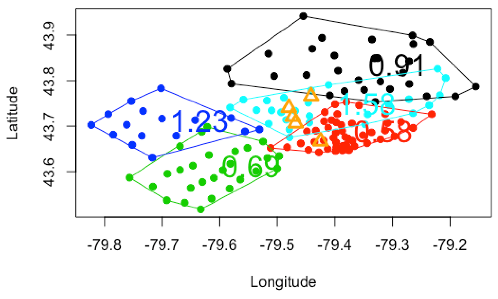
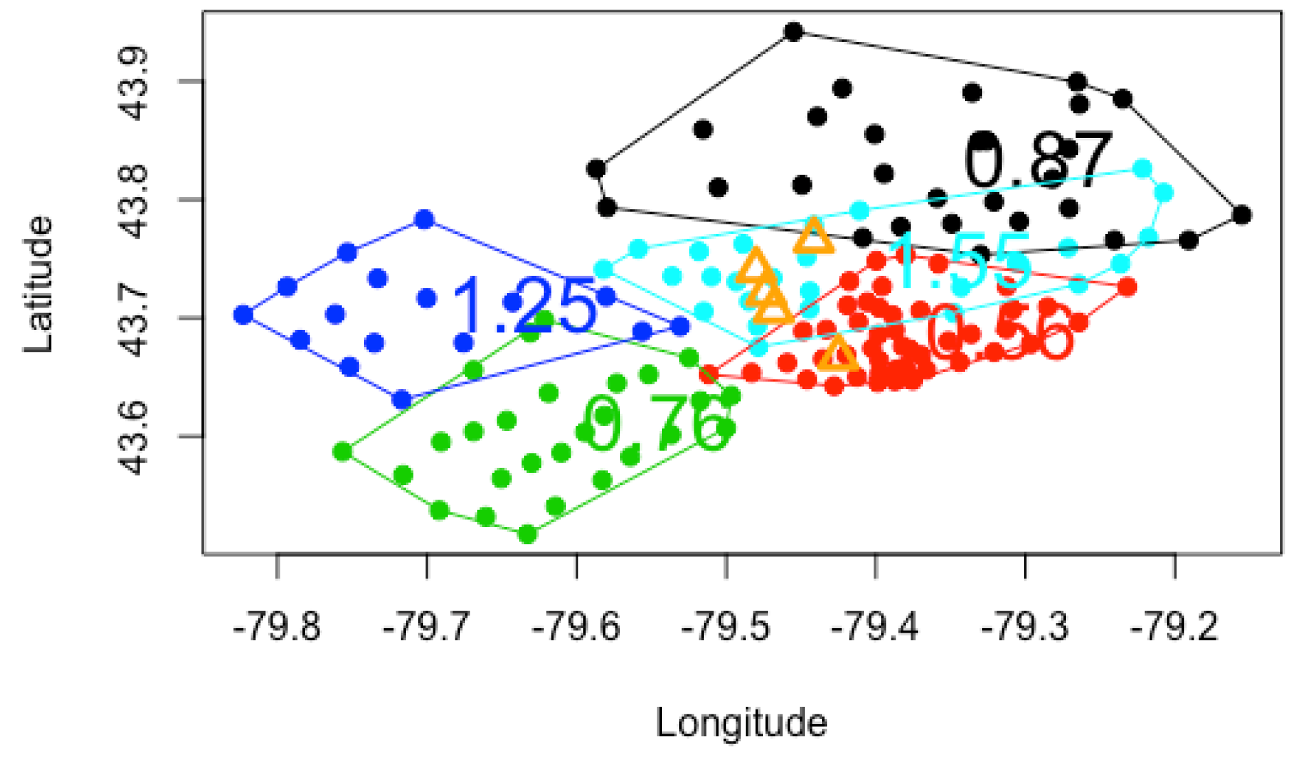
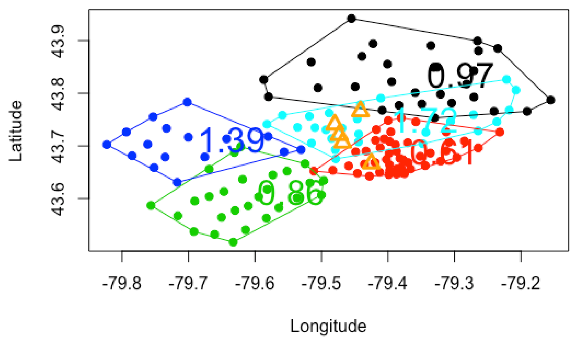
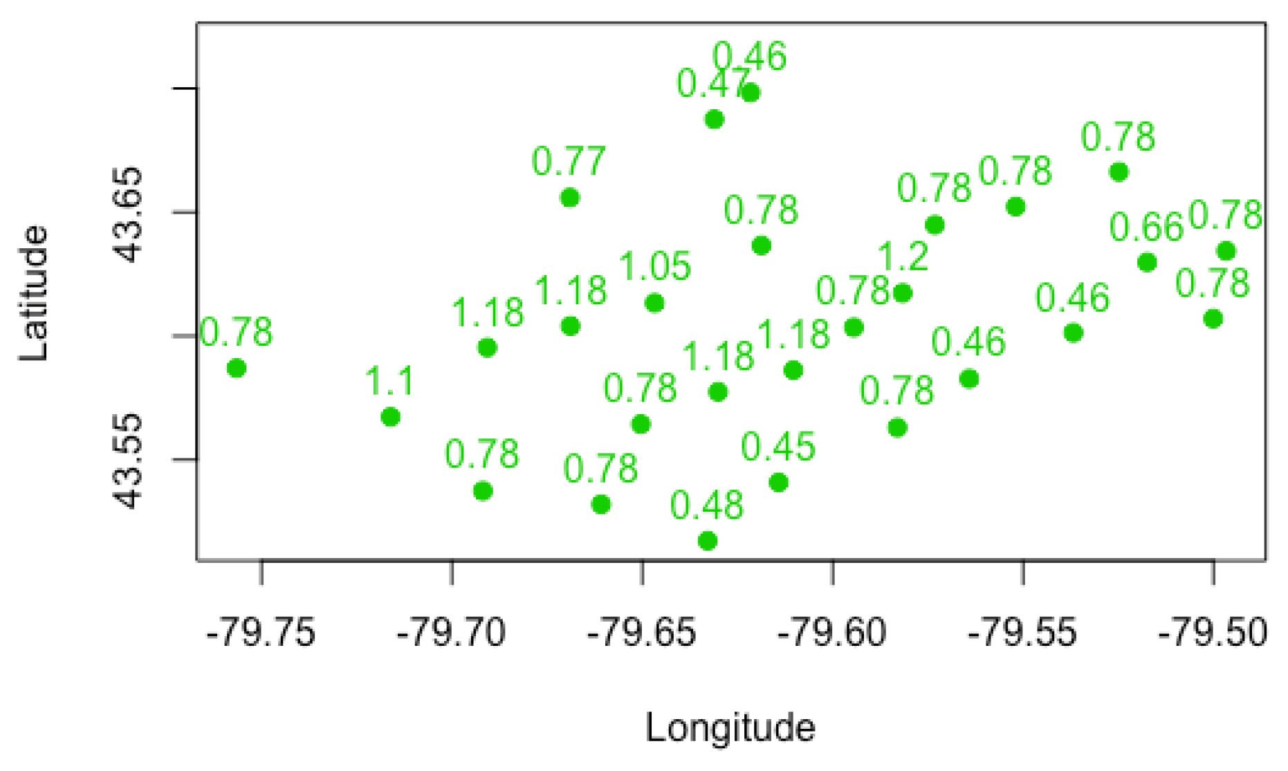
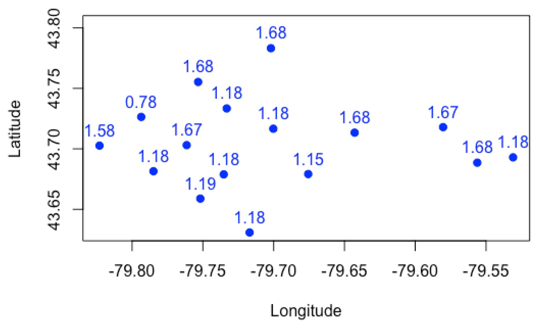
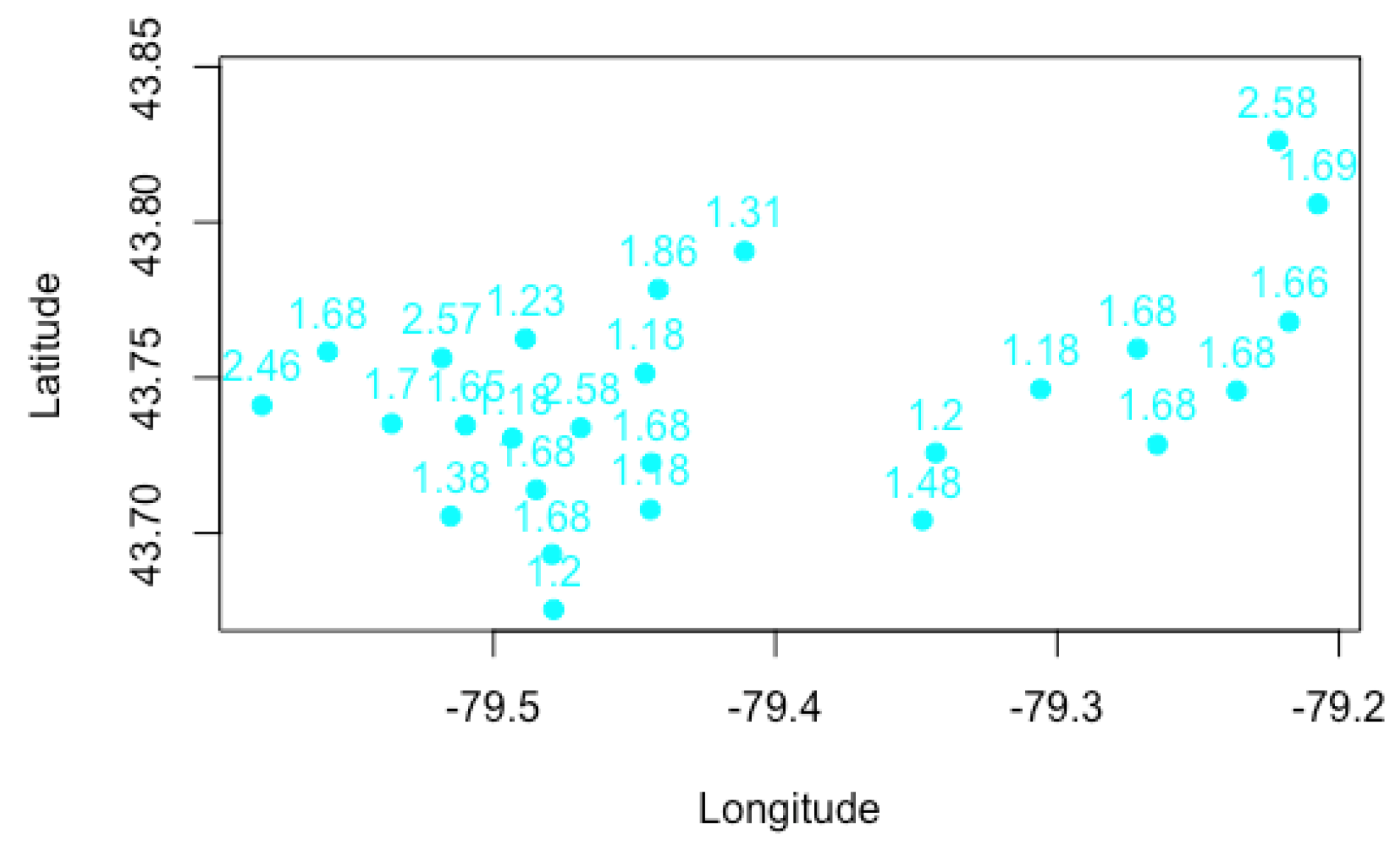
We present plots in Figure 1, Figure 2 and Figure 3 to visualize the grouping structures and estimated relativities of the obtained clusters. The x-axis represents the longitude, and the y-axis represents the latitude. Using K-Means clustering, we have created homogeneous clusters in terms of relativities, where points within the same cluster boundary share the common information of relativity. Figure 1, Figure 2 and Figure 3 show the results for $K=5$, using the empirical, GLM and GLMM. We find that the estimated relativities among these three methods are not significantly different, and the estimated values appear reasonable. For instance, for $K=5$, the relativities in the blue and light blue clusters are higher than those of the red and green clusters, indicating that the North York and Brampton regions have a higher risk than the Etobicoke and Mississauga regions. This observation can be explained by the different driving behaviors and traffic volumes in these districts. However, the generalized linear mixed model gave slightly higher relativities in each cluster, possibly leading to the overestimation of the pure premium. Nevertheless, this method considers the spatial random effect of cities, making it more suitable for certain applications.

Increasing the number of clusters can improve the accuracy and specificity of risk assessment by considering smaller cluster boundaries. Some FSA do not need to be evaluated in the same risk category. For instance, the black cluster in Figure 2 ($K=5$) can be partitioned into multiple clusters if we set $K=10$. Another noteworthy observation is that the overlaps between clusters decrease as the number of clusters increases. We prefer well-separated groups because they provide less ambiguity in defining the relativities of other FSA within the cluster boundaries. However, if we allow too many clusters, the model can overfit the data and become meaningless by assigning each FSA using its own risk relativity. A regulator must balance the complexity of the groups with the geographical information available. Although the selection of the optimal number of clusters is often based on the sum of squares data variation, our experiments reveal that this approach produces a small number of clusters with little relevance to the actual application of territory risk classification.

Figure 1, Figure 2 and Figure 3 show the cluster centers from fuzzy C-Means clustering. When using fuzzy clustering, we observe that the cluster center is shifted toward the center of all FSA because each FSA is associated with all clusters. In K-Means clustering, we assume the same risk relativity for each FSA within the same group, which may not be sufficient for rate regulation purposes, as each FSA may have its own risk level, particularly for the FSA with a sufficiently large number of risk exposures. In this case, the relativity of such FSA is considered representative and they must be differentiated from others. We further investigate how fuzzy C-Means clustering leads to different results. For this study, we first set up combinations of the two main parameters of fuzzy C-Means clustering. The number of clusters (C) ranges from 5 to 30, and the value of the fuzziness coefficient (m) varies between 1 and 3 at an increment of 0.1. The estimated risk relativity for each run is produced according to its membership coefficient matrix. By comparing the RMSE and MAD of the relativities, we select $m=1.4$ as the optimal fuzziness. Note that the results below were produced based on $m=1.4$.

Table 3. The membership coefficients from five-cluster fuzzy C-Means clustering. The bold value indicates the dominant cluster for the selected FSA that we used for illustration purposes.

FSA-ID	Cluster 1	Cluster 2	Cluster 3	Cluster 4	Cluster 5
1	0.0039	0.0003	0.0007	0.0001	0.9950
2	0.9835	0.0013	0.0047	0.0003	0.0102
3	0.0245	0.8135	0.1405	0.0102	0.0113
4	0.9994	0.0001	0.0002	0.0000	0.0003
5	0.9910	0.0007	0.0027	0.0002	0.0054
6	0.9315	0.0070	0.0344	0.0014	0.0257
7	0.9989	0.0001	0.0004	0.0000	0.0006
8	0.0083	0.0058	0.9829	0.0006	0.0024
9	0.4262	0.0484	0.4545	0.0074	0.0635
10	0.7713	0.0239	0.1437	0.0042	0.0569
11	0.9985	0.0001	0.0006	0.0000	0.0008
12	0.9987	0.0001	0.0005	0.0000	0.0007
13	0.0247	0.8120	0.1417	0.0103	0.0114
14	0.0868	0.0118	0.0254	0.0039	0.8720
15	0.9912	0.0008	0.0036	0.0002	0.0043
16	0.0351	0.0954	0.8509	0.0057	0.0130
17	0.9984	0.0001	0.0006	0.0000	0.0008
18	0.5525	0.0422	0.3307	0.0068	0.0679
19	0.0430	0.0205	0.9232	0.0023	0.0110
20	0.1546	0.0419	0.7653	0.0054	0.0328

,

Table 4. The membership coefficients from six-cluster fuzzy C-Means clustering. The bold value indicates the dominant cluster for the selected FSA that we used for illustration purposes.

FSA-ID	Cluster 1	Cluster 2	Cluster 3	Cluster 4	Cluster 5	Cluster 6
1	0.0676	0.0045	0.0117	0.0006	0.9136	0.0020
2	0.8473	0.0162	0.0912	0.0012	0.0390	0.0050
3	0.0292	0.4298	0.0721	0.0142	0.0165	0.4382
4	0.6641	0.0334	0.2340	0.0023	0.0565	0.0097
5	0.8134	0.0197	0.1155	0.0015	0.0439	0.0060
6	0.3118	0.0488	0.5769	0.0028	0.0472	0.0125
7	0.6536	0.0343	0.2430	0.0023	0.0570	0.0099
8	0.0394	0.6450	0.2639	0.0041	0.0163	0.0313
9	0.0033	0.0039	0.9912	0.0001	0.0009	0.0006
10	0.0758	0.0284	0.8721	0.0013	0.0161	0.0063
11	0.6457	0.0349	0.2498	0.0024	0.0572	0.0100
12	0.6483	0.0347	0.2475	0.0024	0.0572	0.0100
13	0.0292	0.4317	0.0722	0.0142	0.0165	0.4362
14	0.0802	0.0122	0.0256	0.0021	0.8740	0.0060
15	0.5642	0.0407	0.3224	0.0027	0.0587	0.0114
16	0.0011	0.9914	0.0041	0.0002	0.0005	0.0027
17	0.6430	0.0351	0.2521	0.0024	0.0573	0.0101
18	0.0017	0.0014	0.9962	0.0000	0.0004	0.0002
19	0.0527	0.4171	0.4744	0.0044	0.0205	0.0309
20	0.0443	0.1485	0.7724	0.0026	0.0155	0.0166

and

Table 5. The membership coefficients from ten-cluster fuzzy C-Means clustering. The bold value indicates the dominant cluster for the selected FSA that we used for illustration purposes.

FSA-ID	Cluster 1	Cluster 2	Cluster 3	Cluster 4	Cluster 5	Cluster 6	Cluster 7	Cluster 8	Cluster 9	Cluster 10
1	0.0120	0.0022	0.0049	0.0002	0.7771	0.0006	0.1585	0.0323	0.0012	0.0109
2	0.6325	0.0069	0.0292	0.0004	0.0158	0.0011	0.0454	0.2618	0.0028	0.0041
3	0.0026	0.0197	0.0049	0.0007	0.0011	0.0054	0.0014	0.0018	0.9616	0.0007
4	0.9737	0.0010	0.0048	0.0000	0.0015	0.0001	0.0037	0.0143	0.0004	0.0004
5	0.7338	0.0060	0.0260	0.0003	0.0125	0.0009	0.0348	0.1801	0.0023	0.0034
6	0.8086	0.0112	0.0864	0.0005	0.0096	0.0014	0.0206	0.0549	0.0037	0.0032
7	0.9803	0.0007	0.0037	0.0000	0.0011	0.0001	0.0028	0.0106	0.0003	0.0003
8	0.0363	0.7155	0.1597	0.0017	0.0086	0.0071	0.0129	0.0194	0.0345	0.0043
9	0.0001	0.0001	0.9997	0.0000	0.0000	0.0000	0.0000	0.0000	0.0000	0.0000
10	0.3273	0.0317	0.5129	0.0010	0.0154	0.0031	0.0295	0.0642	0.0092	0.0057
11	0.9846	0.0006	0.0030	0.0000	0.0009	0.0001	0.0022	0.0082	0.0002	0.0003
12	0.9832	0.0006	0.0032	0.0000	0.0010	0.0001	0.0024	0.0089	0.0002	0.0003
13	0.0027	0.0202	0.0050	0.0007	0.0011	0.0056	0.0015	0.0019	0.9606	0.0007
14	0.0326	0.0094	0.0174	0.0013	0.4828	0.0030	0.1193	0.0591	0.0055	0.2696
15	0.9989	0.0000	0.0003	0.0000	0.0001	0.0000	0.0001	0.0005	0.0000	0.0000
16	0.0124	0.8682	0.0319	0.0014	0.0040	0.0069	0.0056	0.0078	0.0597	0.0022
17	0.9859	0.0005	0.0028	0.0000	0.0008	0.0001	0.0020	0.0074	0.0002	0.0002
18	0.0280	0.0092	0.9434	0.0002	0.0025	0.0007	0.0044	0.0084	0.0022	0.0010
19	0.0626	0.4502	0.3660	0.0023	0.0132	0.0089	0.0202	0.0315	0.0388	0.0063
20	0.0608	0.1410	0.7125	0.0014	0.0104	0.0052	0.0166	0.0272	0.0201	0.0047

show the membership coefficients of clusters for 20 selected FSA as the number of clusters used for clustering changes. These results reveal the evolution of the coefficients and highlight a strong connection between them. For example, when the number of clusters is set to 5, the dominant cluster for the first FSA is cluster 5 with a coefficient of 0.9950. As the number of clusters increases to 6, this coefficient changes to 0.9136 but remains the most dominant. However, when the number of clusters becomes 10, this coefficient decreases to 0.7771. The dominant clusters for the selected FSA are displayed in bold in Table 3, Table 4 and Table 5. We present the results for the first 20 FSA out of 155, and we observe a consistent changing pattern as the number of clusters increases. However, increasing the number of clusters also increases the uncertainty in the FSA membership in a given cluster. Nonetheless, we find that they exhibit similar behavior in terms of risk relativity, indicating the robustness of the fuzzy approach in estimating and smoothing the risk relativity across all FSA.

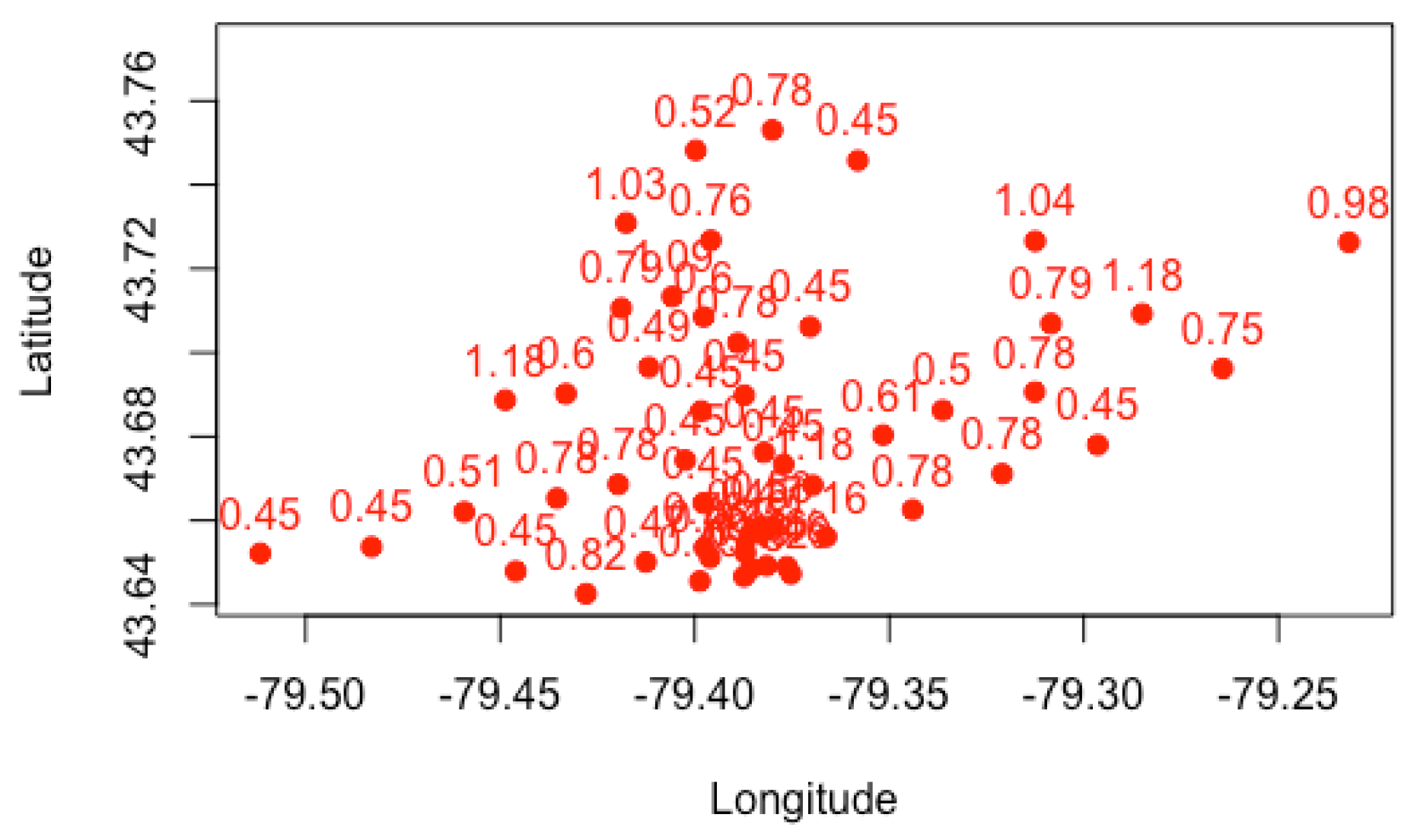
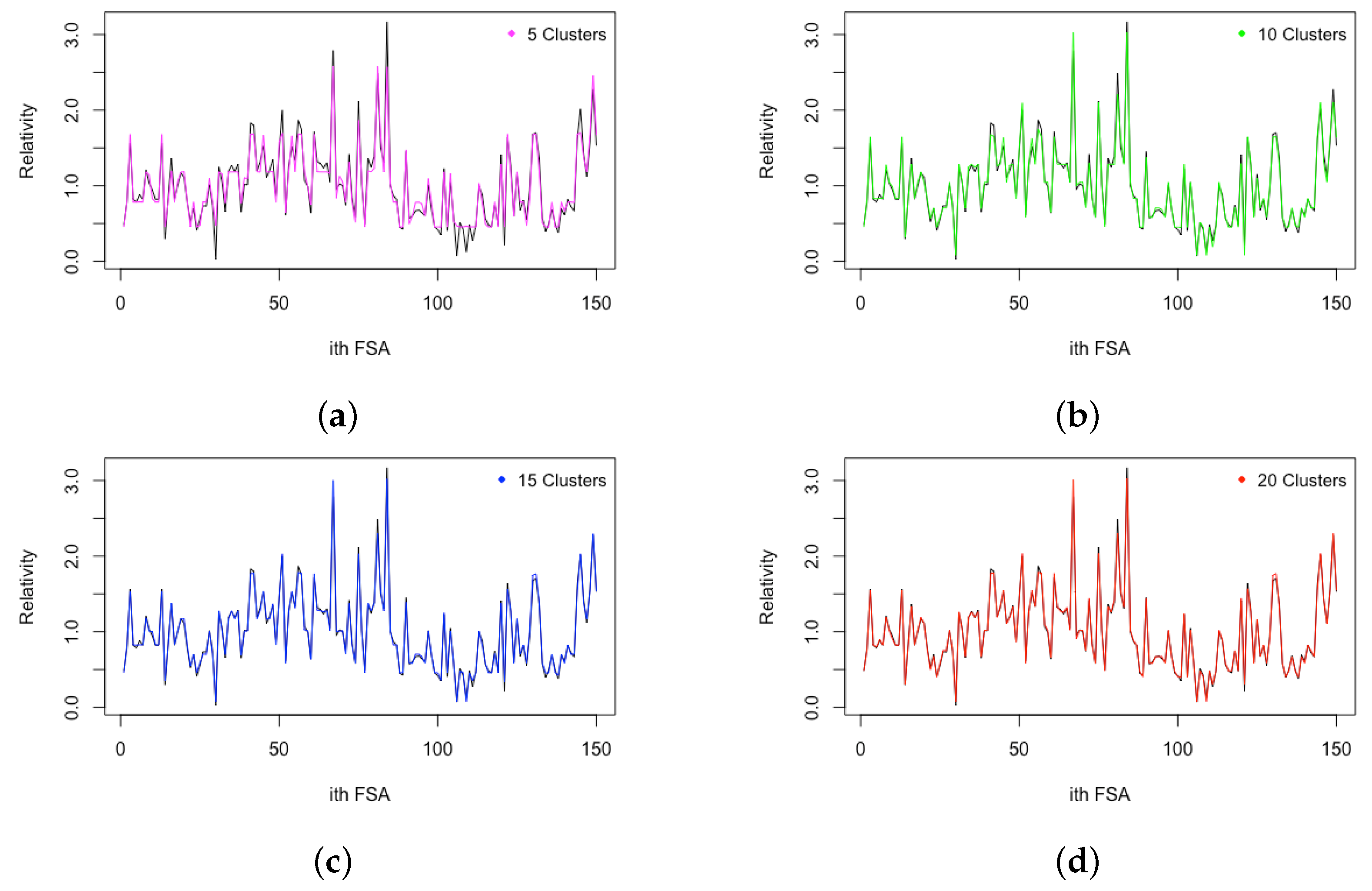
Figure 4, Figure 5, Figure 6, Figure 7 and Figure 8 show that although a cluster is defined by K-Means clustering, many FSA within the group have different risk relativities. However, some FSA within the same cluster have similar values of risk relativity. This highlights the flexibility of fuzzy C-Means clustering in estimating the risk relativity for FSA within the same cluster. Moreover, different clusters have different values of risk relativity, and, within the same group, the FSA can also have different values of risk relativity when using fuzzy C-Means clustering. We display the results for a case with a smaller cluster for visualization purposes; in practice, the number of clusters may be large, so as to improve the heterogeneity of groups. In fact, the risk relativity shown in these figures can be further refined to make them less discriminatory when this is desirable. For instance, controlling the number of major principal components retained can lead to refinement when applying principal component analysis. Our work in Xie and Gan (2022) shows the evolution of the risk relativity when the number of principal components is changed, and, when all principal components are retained, the result becomes the same as the one presented in this work (i.e., Figure 7 becomes the same as Figure 4d in Xie and Gan (2022)).

The fact that different FSA within the same cluster can have different values of risk relativity is advantageous over K-Means clustering and GLMM, as it provides a way to reflect the potential risk heterogeneity. In addition, it is worth noting that the estimation of risk relativity for each FSA is based on the results from all clusters, making the estimates more robust. In Figure 9, we present the FSA risk relativity estimates based on fuzzy C-Means clustering for different numbers of clusters. 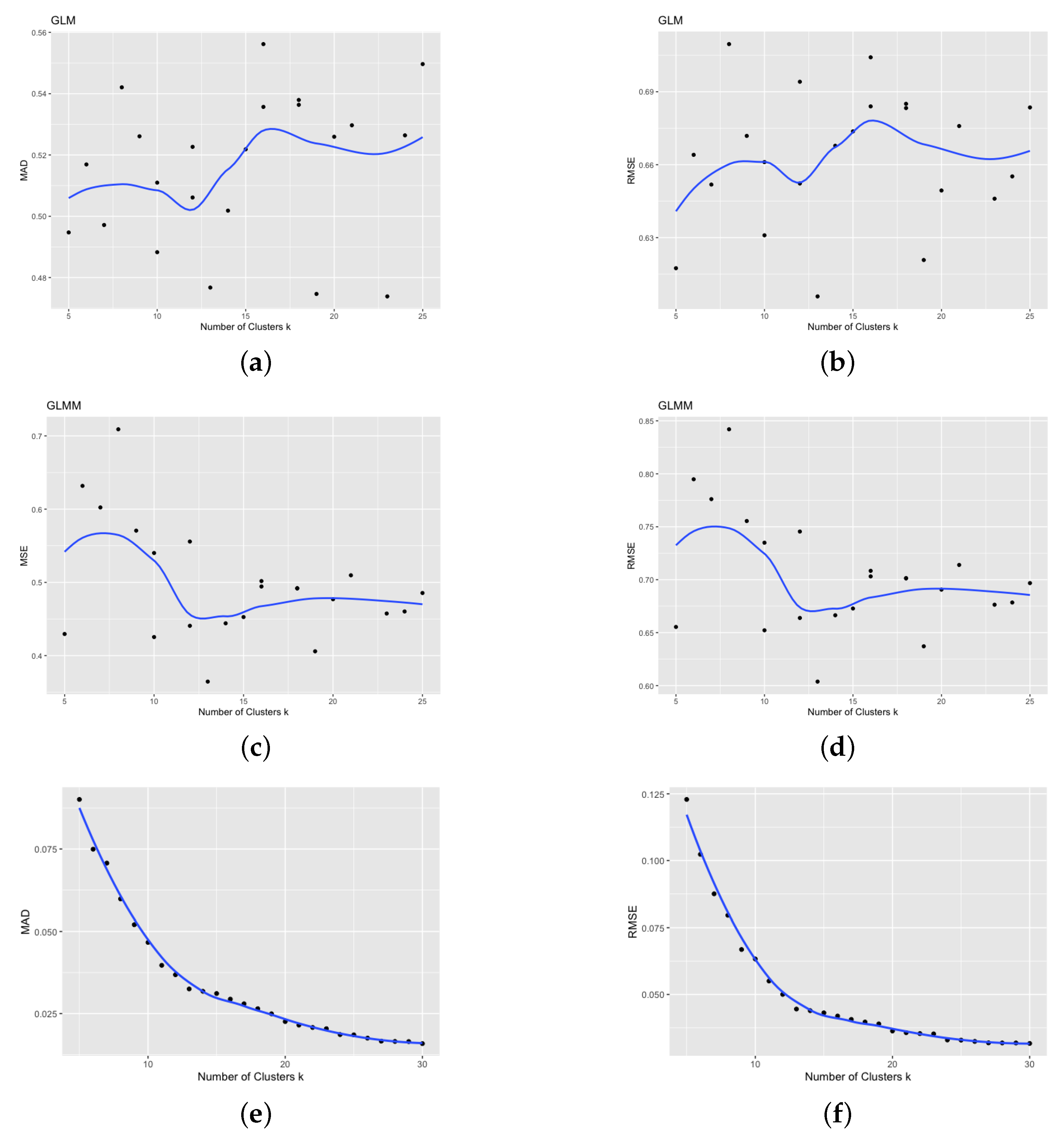The results indicate that the estimate of FSA risk relativity is robust to the number of clusters, unlike in the case of K-Means clustering. Moreover, Figure 10 shows that increasing the number of groups in fuzzy C-Means clustering leads to a decreased RMSE or MAD. In contrast, the RMSE or MAD is significantly higher in K-Means clustering, and the decreasing pattern is not apparent when using GLM or GLMM. These findings suggest that fuzzy clustering outperforms K-Means clustering and GLMM. Finally, the plot in Figure 10 shows the values of RMSE and MAD for different numbers of clusters and models/approaches, providing further evidence of the superior performance of fuzzy clustering.

5. Concluding Remarks

Generalized linear and generalized linear mixed models have become increasingly popular in insurance pricing and other areas involving predictive modeling techniques, particularly in auto insurance rate making. While GLM and GLMM have been used as modern actuarial statistical techniques for insurance pricing, they have yet to be extensively explored for rate regulation purposes. In this work, we proposed to use GLMM to estimate the risk relativities after obtaining a set of territories from geographical auto insurance loss cost data. Our study illustrated that GLMM are an appropriate model in assessing the risk associated with the obtained clusters. Within this approach, we first implemented spatially constrained clustering to produce more homogeneous groups to obtain the clusters. GLMM were then used to model the loss cost by explaining the variation and by capturing fixed and random effects. The results suggest that GLMM are promising in estimating the risk relativity for spatially constrained clustering with an optimal number of clusters. This approach can help insurance companies to better understand and manage the risks associated with geographical areas and ultimately improve their pricing strategies. By incorporating spatially constrained clustering and GLMM, we can gain a more accurate and insightful understanding of the underlying risk factors and make more informed decisions in insurance rate regulation.

In this work, we further investigated the impact of soft clustering, specifically fuzzy clustering, on the estimation of territory risk relativities, compared to hard clustering methods such as K-Means clustering. We found that fuzzy C-Means clustering provides a more robust approach to estimating the FSA risk relativity as the results are not influenced significantly when we increase the number of clusters. Moreover, the fuzzy clustering approach leads to a different estimate of the FSA risk relativity, unlike the K-Means method, where the FSA risk relativity is the same within the same cluster. Therefore, by increasing the number of designed territories (i.e., clusters) using fuzzy clustering, one can achieve greater heterogeneity of the FSA risk. We also observed that while fuzzy clustering yields more heterogeneity, it still exhibits some smoothing errors, as seen in both the root mean square error (RMSE) and mean absolute deviation (MAD). However, these errors decrease as we increase the number of clusters. Overall, fuzzy C-Means clustering is a promising method in estimating territory risk relativities, especially compared to traditional hard clustering methods such as K-Means clustering.

From a rate regulation perspective, regulators must stay up-to-date with rapid technological advancements and remain informed about the latest state-of-the-art techniques. This is important to ensure that their regulations remain relevant and up-to-date. As machine learning continues to evolve, regulators may need to adjust their guidelines to ensure that insurers use these techniques competently and responsibly. As machine learning algorithms become increasingly complex, regulators may need to develop more sophisticated approaches to evaluate and monitor the use of these techniques in the insurance industry. From a data modeling perspective, our work focused on using the loss cost instead of separating the risks by severity and frequency. This is because reconciling clustering results by severity and frequency is challenging and more volatile from period to period. Moreover, we considered only the special cases of Tweedie distribution to allow a better understanding of the error distributions used.

The main difference between our work and other studies is that we focused on soft clustering rather than a hard one for territory design. When estimating the risk relativity of FSA, we incorporated another variable’s fixed effect to make the relativity estimate more practical and relevant. Furthermore, we addressed the problem from a rate regulation perspective rather than individual company pricing. The main contribution of the empirical results is to demonstrate that the newly proposed method can offer an alternative approach for territory design and risk analysis. However, interpretable methods are preferred in rate regulation practice. Since fuzzy C-Means clustering is more advanced and technically complicated than K-Means clustering, regulators may be uncomfortable when replacing the existing method with the new one, although our study has demonstrated that the proposed methods are statistically sound. To overcome this difficulty, future work will continue to investigate other soft clustering methods to obtain a more in-depth understanding of the differences and connections between hard clustering and soft clustering. Moreover, the sparsity constraint may be introduced to remove the small membership coefficients, and the membership coefficient matrix can be reconstructed after the sparsity constraint is applied. This idea may help us to understand the connections between fuzzy clustering and K-Means.