
A Non-Performing Loans (NPLs) Portfolio Pricing Model Based on Recovery Performance: The Case of Greece
Abstract
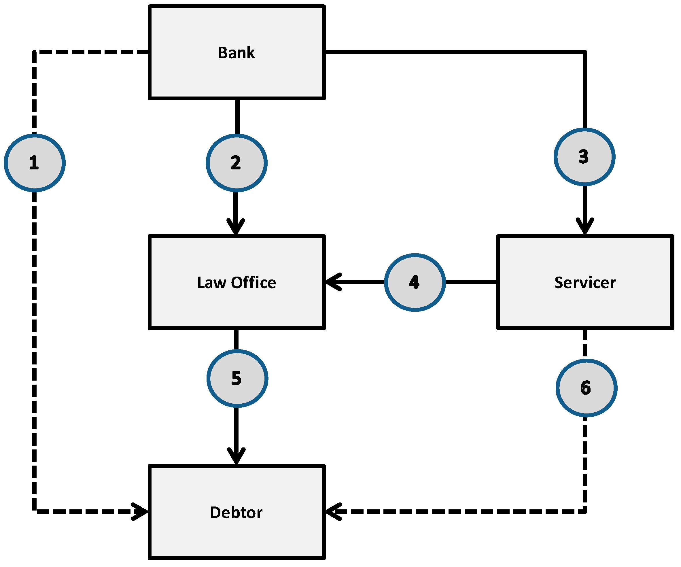
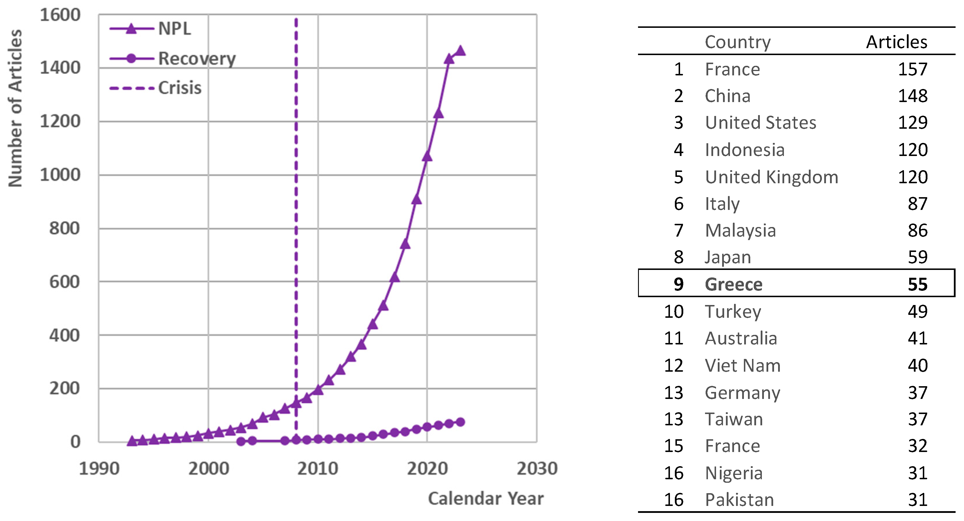
:1. Introduction
- (1)
- By in-house collection;
- (2)
- By being assigned to a legal agency for collection; or
- (3)
- By selling to a servicer.
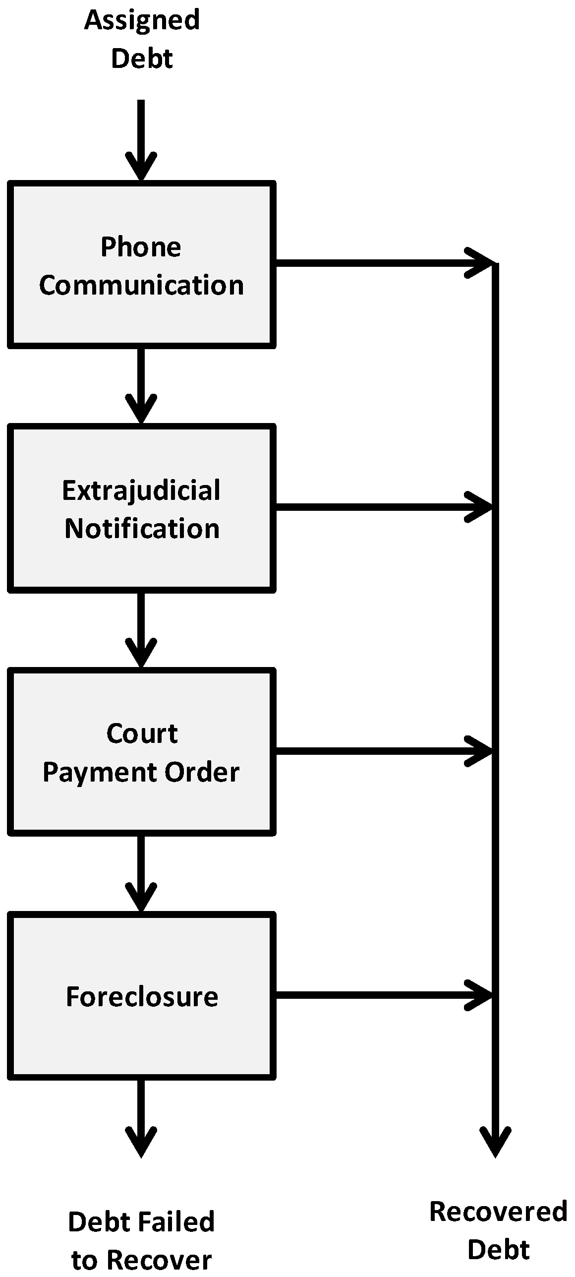
2. Process Description
- Phone communication and discussion with the debtor;
- Extrajudicial notification of the debt and debtor obligations;
- Court order of payment;
- Foreclosure in the case of existing real estate properties.
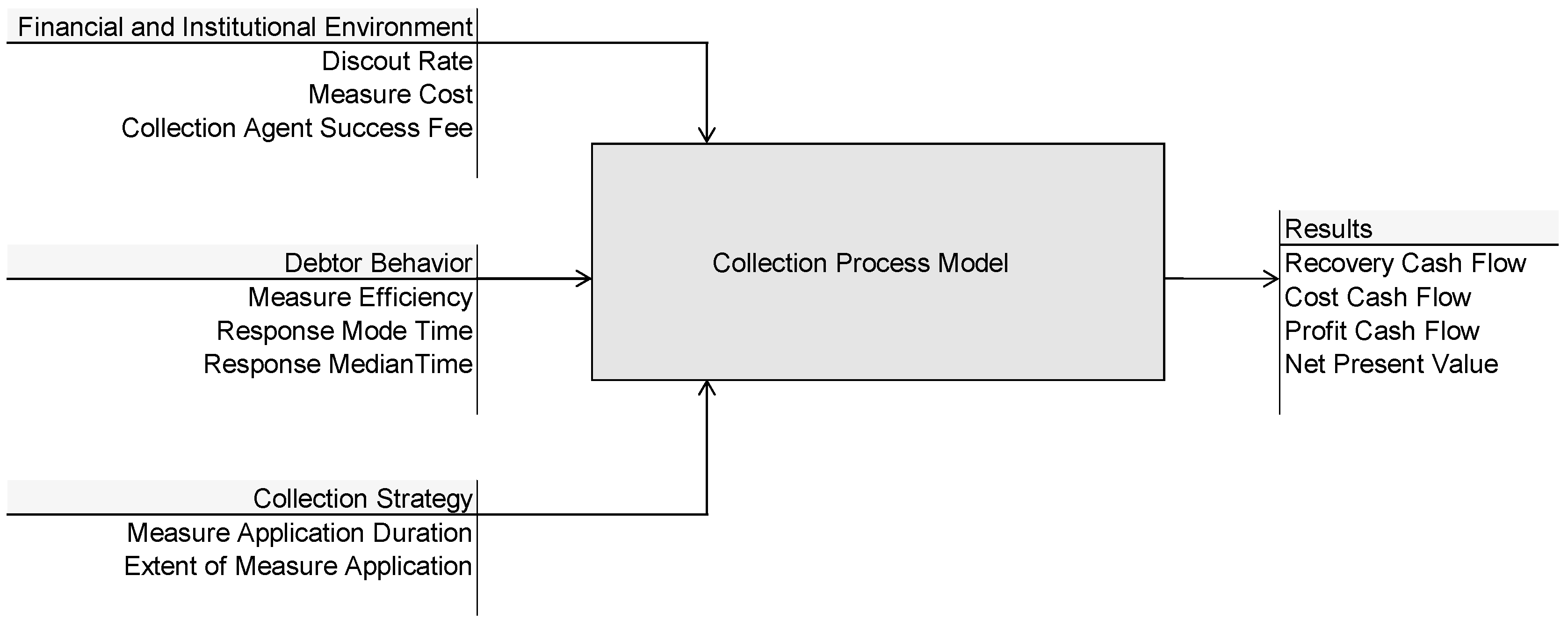
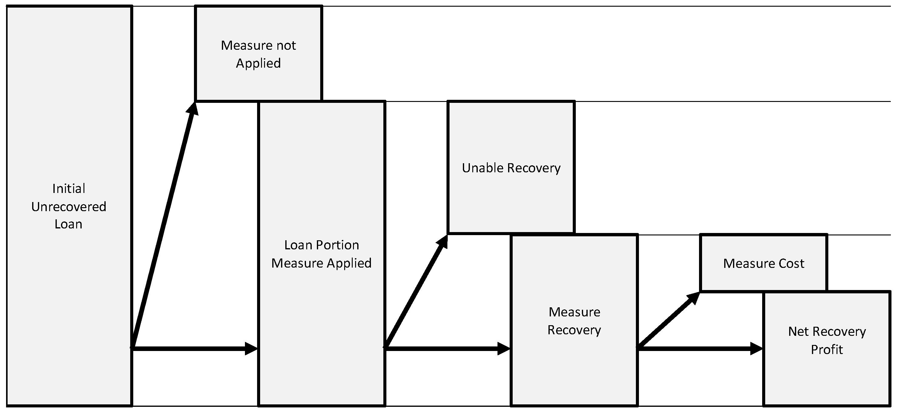
3. Process Model
3.1. Targets
- The recovery cash flow;
- The measure cost cash flow;
- The profit cash flow;
- The NPL portfolio Net Present Value.
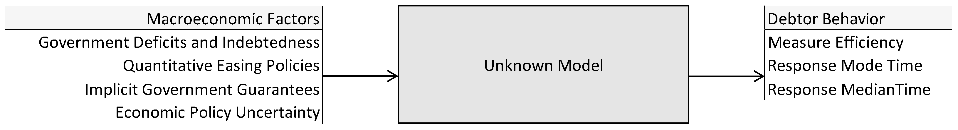
3.2. Factors
- The discount rate, which expresses the time value of money;
- The measure cost, which refers to various measure application costs;
- The success fee for the collection agency.
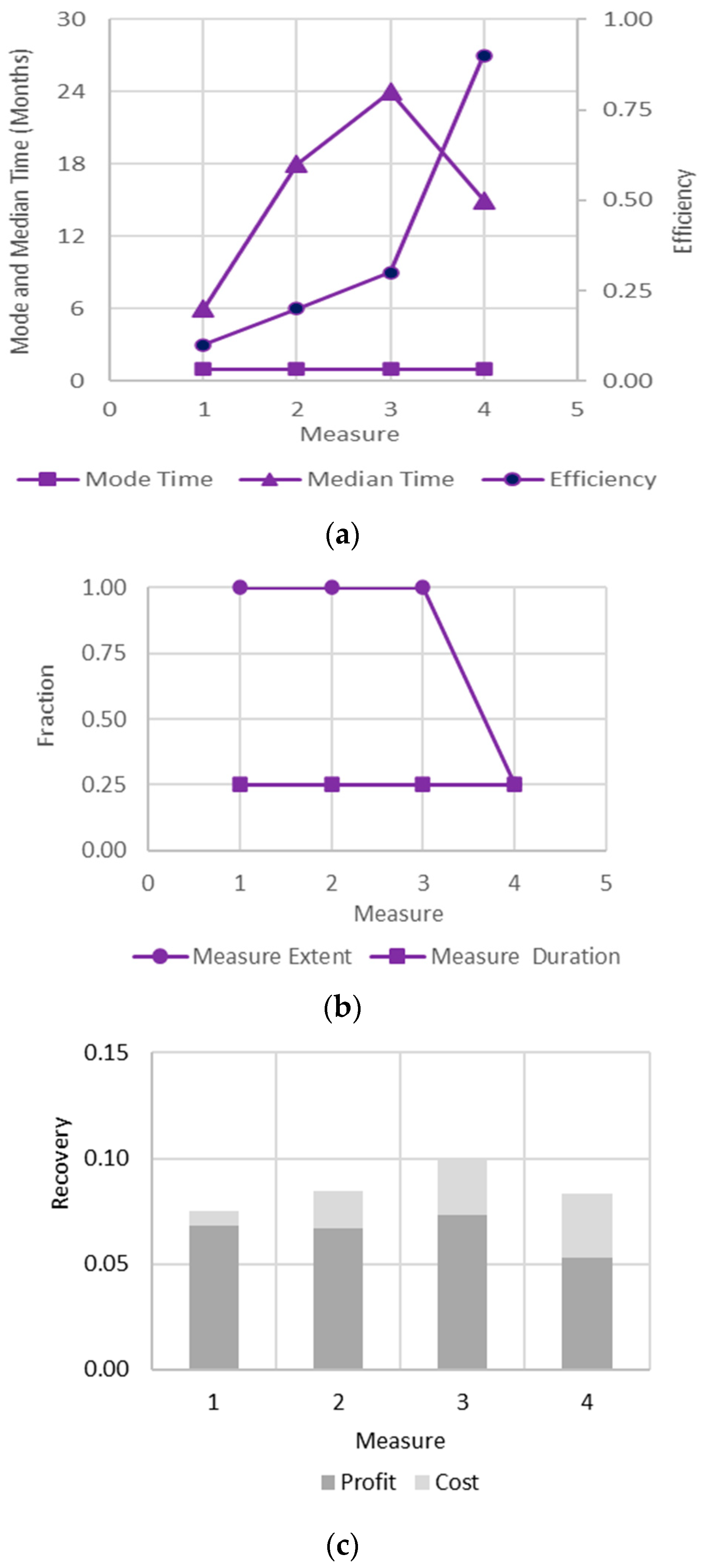
- The measure efficiency;
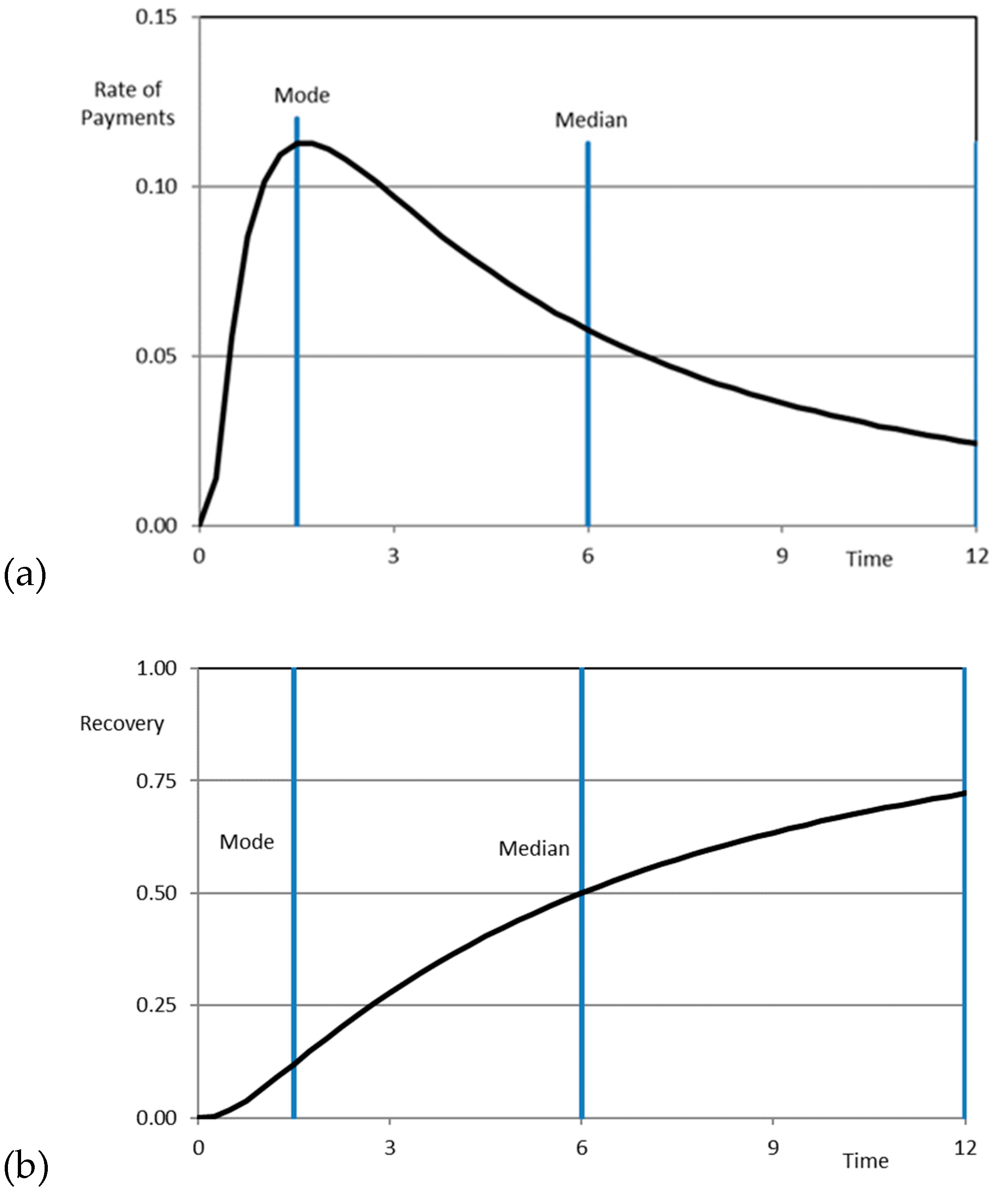
- The mode debtor response time;
- The median debtor response time.
- The debt fraction for which the measure is applied;
- The time interval for which the measure is kept active.
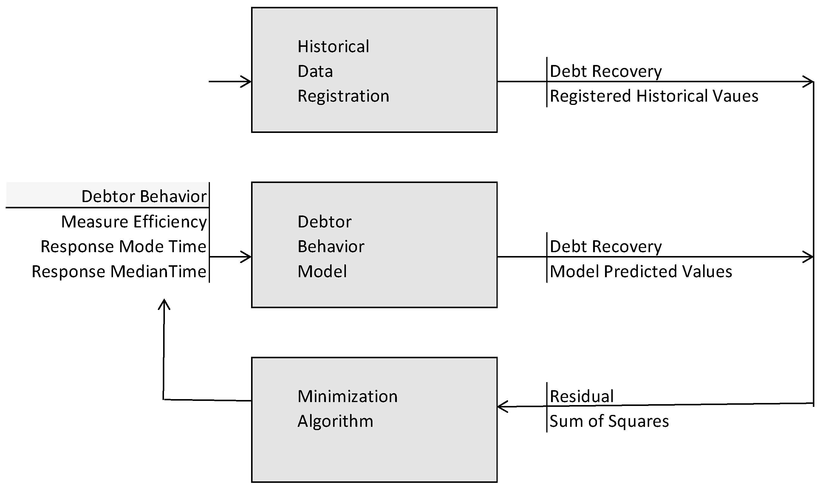
3.3. Parameter Estimation
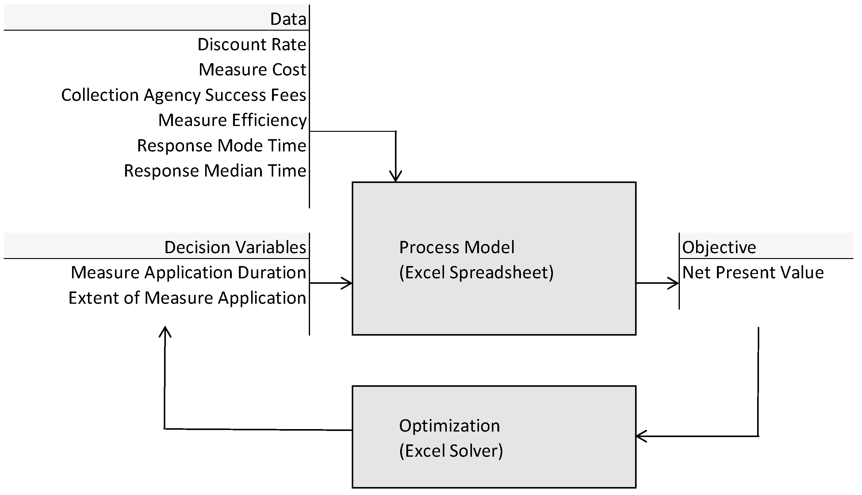
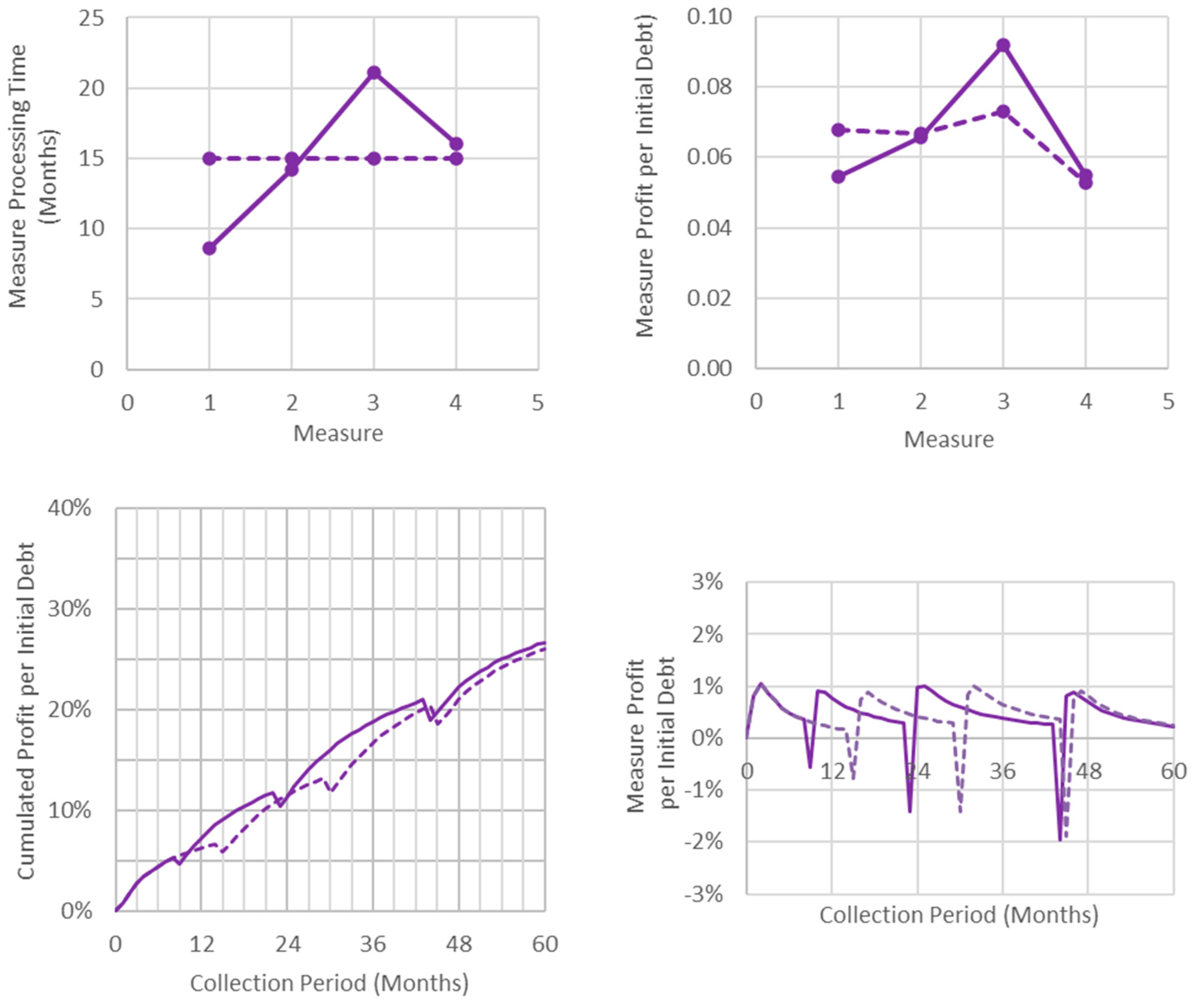
3.4. Process Optimization
- The extent of measure application (the debt fraction for which the measure is applied);
- The measurement duration (the time interval for which the measure is kept active).
3.5. Model Equations
3.6. The Case of Greece
4. Results and Discussion
4.1. Base Case
- The NPL portfolio consisted of personal loans and credit cards;
- The size of the loans had a medium average of about EUR 7500/case;
- Collaterals existed for 25% of the loans;
- Cost data were according to recently updated Greek legislation;
- Debtors’ behavior was according to the period of economic expansion in Greece;
- The collection period of 5 years was divided equally into 15 months per measure;
- The time value of money was 10% discount rate.
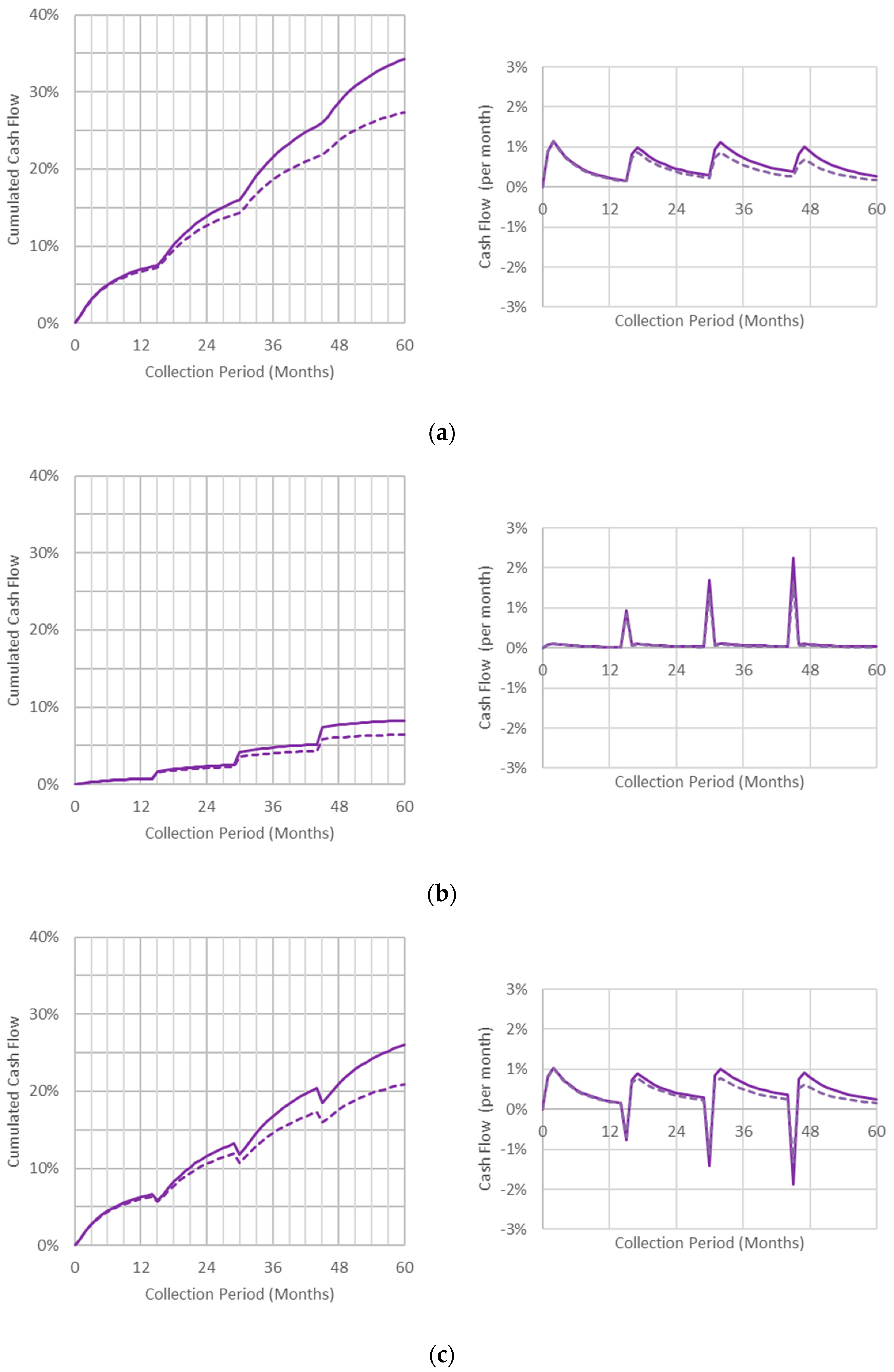
4.2. Optimization
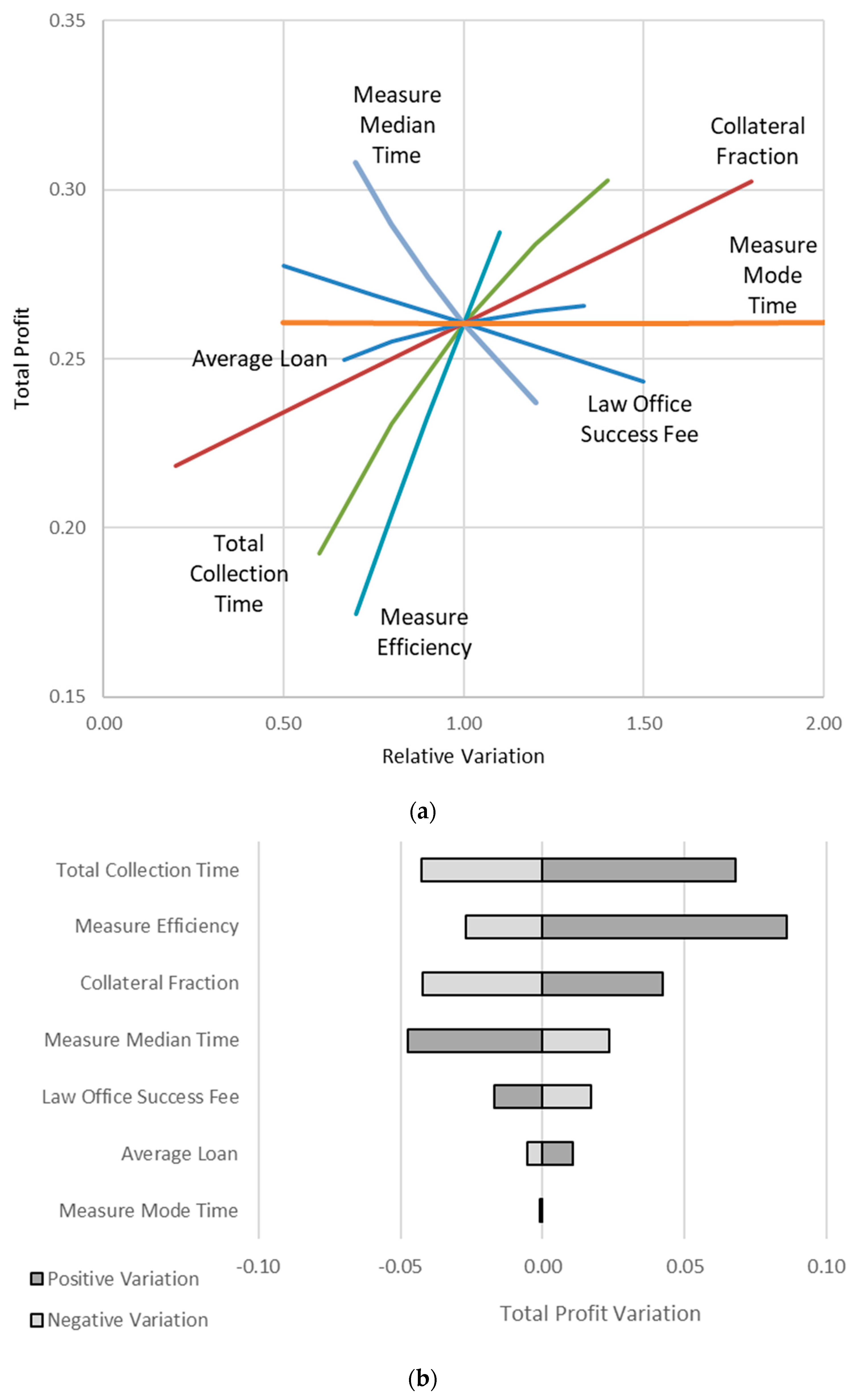
4.3. Sensitivity Analysis
- Debt Characteristics
- Debtors Behavior
- Cost Data
- Collection Strategy
5. Conclusions
Author Contributions
Funding
Data Availability Statement
Acknowledgments
Conflicts of Interest
References
- Alihodžić, Almir, and İbrahim Halil Ekşï. 2018. Credit growth and non-performing loans: Evidence from turkey and some balkan countries. Eastern Journal of European Studies 9: 229–49. [Google Scholar]
- Baker, Scott R., Nicholas Bloom, and Steven J. Davis. 2016. Measuring Economic Policy Uncertainty. The Quarterly Journal of Economics 131: 1593–636. [Google Scholar] [CrossRef]
- Beck, Roland, Petr Jakubik, and Anamaria Piloiu. 2015. Key determinants of non-performing loans: New evidence from a global sample. Open Economies Review 26: 525–50. [Google Scholar] [CrossRef]
- Bellotti, Anthony, Damiano Brigo, Paolo Gambetti, and Frédéric Vrins. 2021. Forecasting recovery rates on non-performing loans with machine learning. International Journal of Forecasting 37: 428–44. [Google Scholar] [CrossRef]
- Blanchard, Olivier, and Pedro Portugal. 2017. Boom, slump, sudden stops, recovery, and policy options. portugal and the euro. Portuguese Economic Journal 16: 149–68. [Google Scholar] [CrossRef]
- Bloom, Nicholas. 2009. The Impact of Uncertainty Shocks. Econometrica 77: 623–85. [Google Scholar] [CrossRef]
- Bolognesi, Enrica, Cristiana Compagno, Stefano Miani, and Roberto Tasca. 2020a. Non-performing loans and the cost of deleveraging: The italian experience. Journal of Accounting and Public Policy 39: 106786. [Google Scholar] [CrossRef]
- Bolognesi, Enrica, Patrizia Stucchi, and Stefano Miani. 2020b. Are NPL-backed securities an investment opportunity? Quarterly Review of Economics and Finance 77: 327–39. [Google Scholar] [CrossRef]
- Calabrese, Raffaella, and Michele Zenga. 2008. Measuring loan recovery rate: Methodology and empirical evidence. Statistica e Applicazioni 6: 193–214. [Google Scholar]
- Campello, Murillo, Gustavo S. Cortes, Fabrício d’Almeida, and Gaurav Kankanhalli. 2022. Exporting Uncertainty: The Impact of Brexit on Corporate America. Journal of Financial and Quantitative Analysis 57: 3178–22. [Google Scholar] [CrossRef]
- Carleo, Alessandra, Roberto Rocci, and Maria Sole Staffa. 2023. Measuring the recovery performance of a portfolio of NPLs. Computation 11: 29. [Google Scholar] [CrossRef]
- Carpinelli, Luisa, Giuseppe Cascarino, Silvia Giacomelli, and Valerio Vacca. 2017. The management of non-performing loans: A survey among the main italian banks. Politica Economica 33: 157–87. [Google Scholar] [CrossRef]
- Chaibi, Hasna, and Zied Ftiti. 2015. Credit risk determinants: Evidence from a cross-country study. Research in International Business and Finance 33: 1–16. [Google Scholar] [CrossRef]
- Chamboko, Richard, and Jorge M. Bravo. 2016. On the modelling of prognosis from delinquency to normal performance on retail consumer loans. Risk Management 18: 264–87. [Google Scholar] [CrossRef]
- Cortes, Gustavo S., George P. Gao, Felipe B. G. Silva, and Zhaogang Song. 2022. Unconventional Monetary Policy and Disaster Risk: Evidence from the Subprime and COVID–19 Crises. Journal of International Money and Finance 122: 102543. [Google Scholar] [CrossRef]
- Dantas, Manuela M., Kenneth J. Merkley, and Felipe B. G. Silva. 2023. Government Guarantees and Banks’ Income Smoothing. Journal of Financial Services Research 63: 123–73. [Google Scholar] [CrossRef]
- Dimitrios, Anastasiou, Louri Helen, and Tsionas Mike. 2016. Determinants of non-performing loans: Evidence from euro-area countries. Finance Research Letters 18: 116–19. [Google Scholar] [CrossRef]
- Foglia, Matteo. 2022. Non-Performing Loans and Macroeconomics Factor: The Italian Case. Risks 10: 21. [Google Scholar] [CrossRef]
- Ghosh, Amit. 2015. Banking-industry specific and regional economic determinants of non-performing loans: Evidence from US states. Journal of Financial Stability 20: 93–104. [Google Scholar] [CrossRef]
- Girardone, Claudia, Philip Molyneux, and Edward P. M. Gardener. 2004. Analysing the determinants of bank efficiency: The case of italian banks. Applied Economics 36: 215–27. [Google Scholar] [CrossRef]
- Karadima, Maria, and Helen Louri. 2020. Non-performing loans in the euro area: Does bank market power matter? International Review of Financial Analysis 72: 101593. [Google Scholar] [CrossRef]
- Karadima, Maria, and Helen Louri. 2021. Determinants of Non-Performing Loans in Greece: The Intricate Role of Fiscal Expansion. GreeSE Paper No. 160. London: Hellenic Observatory, LSE. [Google Scholar]
- Khairi, Ardhi, Bahri Bahri, and Bhenu Artha. 2021. A Literature Review of Non-Performing Loan. Journal of Business and Management Review 2: 366–73. [Google Scholar] [CrossRef]
- Konstantakis, Konstantinos N., Panayotis G. Michaelides, and Angelos T. Vouldis. 2016. Non-performing loans (NPLs) in a crisis economy: Long-run equilibrium analysis with a real time VEC model for Greece (2001–2015). Physica A: Statistical Mechanics and Its Applications 451: 149–61. [Google Scholar] [CrossRef]
- Li, Geng, Muzi Chen, and Xiaoguang Yang. 2022. Impact of centralized management on recovery rates of credit loans. Paper presented at the Chinese Control Conference, CCC, Hefei, China, July 25–27; pp. 7497–502. [Google Scholar] [CrossRef]
- Louzis, Dimitrios P., Angelos T. Vouldis, and Vasilios L. Metaxas. 2012. Macroeconomic and bank-specific determinants of non-performing loans in greece: A comparative study of mortgage, business and consumer loan portfolios. Journal of Banking and Finance 36: 1012–27. [Google Scholar] [CrossRef]
- Makri, Vasiliki, Athanasios Tsagkanos, and Athanasios Bellas. 2014. Determinants of non-performing loans: The case of eurozone. Panoeconomicus 61: 193–206. [Google Scholar] [CrossRef]
- Manz, Florian, Birgit Müller, and Dirk Schiereck. 2020. The pricing of European non-performing real estate loan portfolios: Evidence on stock market evaluation of complex asset sales. Journal of Business Economics 90: 1087–120. [Google Scholar] [CrossRef]
- Marouli, A. Z., Yannis. D. Caloghirou, and Eugenia. N. Giannini. 2015. Non-performing debt recovery: Effects of the greek crisis. International Journal of Banking, Accounting and Finance 6: 21–36. [Google Scholar] [CrossRef]
- Messai, Ahlem Selma, and Fathi Jouini. 2013. Micro and macro determinants of non-performing loans. International Journal of Economics and Financial Issues 3: 852–60. [Google Scholar]
- Nikolaidou, Eftychia, and Sofoklis D. Vogiazas. 2014. Credit risk determinants for the bulgarian banking system. International Advances in Economic Research 20: 87–102. [Google Scholar] [CrossRef]
- Nikolaidou, Eftychia, and Sofoklis Vogiazas. 2017. Credit risk determinants in sub-saharan banking systems: Evidence from five countries and lessons learnt from central east and south east european countries. Review of Development Finance 7: 52–63. [Google Scholar] [CrossRef]
- Orlando, Giuseppe, and Roberta Pelosi. 2020. Non-performing loans for italian companies: When time matters. an empirical research on estimating probability to default and loss given default. International Journal of Financial Studies 8: 68. [Google Scholar] [CrossRef]
- Perotti, Enrico C. 1993. Bank lending in transition economies. Journal of Banking and Finance 17: 1021–32. [Google Scholar] [CrossRef]
- Saulītis, Andris. 2023. Nudging debtors with non-performing loans: Evidence from three field experiments. Journal of Behavioral and Experimental Finance 37: 100776. [Google Scholar] [CrossRef]
- Scardovi, Claudio. 2015. Holistic Active Management of Non-Performing Loans. Berlin/Heidelberg: Springer, pp. 1–153. [Google Scholar] [CrossRef]
- Stijepović, Ristan. 2014. Recovery and reduction of non-performing loans-podgorica approach. Journal of Central Banking Theory and Practice 3: 101–18. [Google Scholar] [CrossRef]
- Tupayachi, Jose, and Luciano Silva. 2022. Better Efficiency on Non-performing Loans Debt Recovery and Portfolio Valuation Using Machine Learning Techniques. In Production and Operations Management. Edited by Jorge Vargas Florez, Irineu de Brito Junior, Adriana Leiras, Sandro Alberto Paz Collado, Miguel Domingo González Alvarez, Carlos Alberto González-Calderón, Sebastian Villa Betancur, Michelle Rodriguez and Diana Ramirez-Rios. Springer Proceedings in Mathematics & Statistics. Cham: Springer, vol. 391. [Google Scholar] [CrossRef]
- Wang, Siyi, Xing Yan, Bangqi Zheng, Hu Wang, Wangli Xu, Nanbo Peng, and Qi Wu. 2021. Risk and return prediction for pricing portfolios of non-performing consumer credit. Paper presented at the ICAIF 2021—2nd ACM International Conference on AI in Finance, Virtual Event, November 3–5. [Google Scholar]
- Ye, Hui, and Anthony Bellotti. 2019. Modelling recovery rates for non-performing loans. Risks 7: 19. [Google Scholar] [CrossRef]


| Phone | Extrajudicial | Order | Foreclosure | |
|---|---|---|---|---|
| Expansion | ||||
| Recovery (%) | 8.40 | 23.6 | 28.0 | 100 |
| Mode (mo) | 1.48 | 3.20 | 1.34 | 2.54 |
| Median (mo) | 4.44 | 22.8 | 19.1 | 25.2 |
| Recession | ||||
| Recovery (%) | 4.90 | 11.4 | 17.9 | 18.6 |
| Mode (mo) | 0.12 | 1.90 | 0.13 | 2.44 |
| Median (mo) | 1.80 | 11.6 | 43.5 | 12.5 |
| 1. Law Office | ||||||
| 1.1 Success Fees | 15 | % of Recovery | ||||
| 2. Extrajudicial | ||||||
| 2.1 Real Estate Check | 45 | € per Case | ||||
| 2.2 Notification | 30 | € per Case | ||||
| 3. Court Order | ||||||
| 3.1 Court Fees | 1 | % of the Loan | ||||
| 3.2 Lawyer Compensation | 64 | € for Loan less than | 12,000 | € | ||
| 139 | € for Loan between | 12,000 | and | 20,000 | € | |
| 268 | € for Loan greater than | 20,000 | € | |||
| 3.3 Notification | 20 | % of the Loan | ||||
| 4. Foreclosure | ||||||
| 4.1 Registration of Encumbrance | 1.72 | % of the Loan | ||||
| 4.2 Court Fees | 150 | € per Case | ||||
| 4.3 Βailiff Compensation | 53 | € for the loan portion less than | 590 | € | ||
| 2.50 | % for the loan portion between | 590 | and | 6500 | € | |
| 1.00 | % for the loan portion between | 6500 | and | 42,200 | € | |
| 0 | % for the loan portion greater than | 42,200 | € |
| Total Collection | Phone | Extra- Juditial | Court Order | Fore- Closure | Units | |
|---|---|---|---|---|---|---|
| Model Input Data | ||||||
| Case Study | Base Case | |||||
| Average Loan Size | 7500 | €/Case | ||||
| Financial and Institutional Environment | ||||||
| Measure Constant Cost | 0 | 75 | 75 | 150 | €/Case | |
| Measure Variable Cost | 0.00 | 0.00 | 0.01 | 0.10 | % Loan | |
| Collection Agent Success Fee | 0.10 | % Recovery | ||||
| Discount Rate | 0.10 | % | ||||
| Debtors Behavior Characteristics | ||||||
| Efficiency | 0.10 | 0.20 | 0.30 | 0.90 | % | |
| Mode Time | 1 | 1 | 1 | 1 | Months | |
| Median Time | 6 | 18 | 24 | 15 | Months | |
| Collection Strategy | ||||||
| Measure Extent | 1.00 | 1.00 | 1.00 | 0.25 | % | |
| Measure Duration | 0.25 | 0.25 | 0.25 | 0.25 | % Total | |
| Total Collection Processing Time | 60 | Months | ||||
| Model Results | ||||||
| Recovery | 0.343 | 0.075 | 0.085 | 0.100 | 0.083 | % |
| Cost | 0.083 | 0.008 | 0.018 | 0.027 | 0.031 | % |
| Profit | 0.260 | 0.068 | 0.067 | 0.073 | 0.053 | % |
| Net Present Value | 0.209 | % |
Disclaimer/Publisher’s Note: The statements, opinions and data contained in all publications are solely those of the individual author(s) and contributor(s) and not of MDPI and/or the editor(s). MDPI and/or the editor(s) disclaim responsibility for any injury to people or property resulting from any ideas, methods, instructions or products referred to in the content. |
© 2023 by the authors. Licensee MDPI, Basel, Switzerland. This article is an open access article distributed under the terms and conditions of the Creative Commons Attribution (CC BY) license (https://creativecommons.org/licenses/by/4.0/).
Share and Cite
Marouli, A.Z.; Giannini, E.N.; Caloghirou, Y.D. A Non-Performing Loans (NPLs) Portfolio Pricing Model Based on Recovery Performance: The Case of Greece. Risks 2023, 11, 96. https://doi.org/10.3390/risks11050096
Marouli AZ, Giannini EN, Caloghirou YD. A Non-Performing Loans (NPLs) Portfolio Pricing Model Based on Recovery Performance: The Case of Greece. Risks. 2023; 11(5):96. https://doi.org/10.3390/risks11050096
Chicago/Turabian StyleMarouli, Alexandra Z., Eugenia N. Giannini, and Yannis D. Caloghirou. 2023. "A Non-Performing Loans (NPLs) Portfolio Pricing Model Based on Recovery Performance: The Case of Greece" Risks 11, no. 5: 96. https://doi.org/10.3390/risks11050096