1. Introduction
The collapse of Lehman Brothers in 2008 sparked extensive debate about the appropriateness of government intervention to save struggling banks. In the event of a bank’s bankruptcy, the losses are typically borne by stakeholders such as creditors and shareholders. However, if a default is avoided through intervention by an external entity, such as a government, supranational organization, or central bank, the losses are spread among a wider population, such as taxpayers. Despite the Dodd–Frank reforms and Basel regulatory standards, which have helped to reduce risk in the financial sector, this topic remains highly relevant today.
Our paper presents a stochastic model that describes the dynamics of banks and is based on real-world financial assumptions. From a regulatory perspective, banks are required to assess their exposure to risk and maintain enough capital to prevent large losses. This capital serves as a buffer to absorb unexpected losses and maintain the ability to continue lending during times of stress, in order to maintain a stable financial system. The Federal Reserve and the Basel Committee on Banking Supervision have established guidelines and proposals for assessing financial stability, even in adverse scenarios. These requirements are outlined in the Comprehensive Capital Analysis Review (CCAR) for American bank holding companies or foreign bank holdings operating in the United States and in the Fundamental Review of the Trading Book (Basel 3.1). The latter, initially published in January 2016 and revised in January 2019, introduced new proposals for market risk-related capital requirements for banks. In this paper, we investigate the implications of these regulations from the perspective of the government or central bank when a bank does not comply with these capital requirements. We refer readers to the work of Bonollo et al. in
Bonollo et al. (
2018) for a comprehensive examination of the mathematical background of minimum capital requirements and the implementation of the Default risk charge, as well as other references
Bertagna et al. (
2020);
Cardone-Riportella et al. (
2013);
Srivastava and Dashottar (
2020) for further information. To simplify matters, in the following sections, we will refer to the external entity that is expected to support distressed banks as “government”.
From a mathematical perspective, we establish a probabilistic framework based on a standard filtered probability space
, where
is the “real-world” probability measure corresponding to the financial scenario we are analyzing, and the time variable
for a given horizon time
, following the approach proposed by Hugonnier and Morellec in
Hugonnier and Morellec (
2017), see also
Cordoni et al. (
2020) and references therein, in the context of impulsive stochastic control. We assume that banks’ financial assets consist of capital invested in risky assets, liquid reserves
S (such as cash, cash equivalents, marketable securities, and accounts receivable), liabilities
L, and deposits
D. In other words, tangible assets (such as inventories, property, plant, and equipment) and intangible assets (such as goodwill and patents) are not considered in this analysis as the focus is on the financial structure and solvency of the bank. For the sake of simplicity, all risky assets are summarized by a global one,
A, whose dynamics are determined by a drifted Brownian motion and a compound Poisson process
with initial value
, where
, the constants
and
are, respectively, the drift and the volatility of the bank’s asset value,
is the taxation rate paid continuously, and
is a Brownian motion (BM), while
denotes the compound Poisson process, adapted to the filtration
, such that
representing the sequence of random times at which the asset price process
experiences (negative) jumps, hence breaking the continuity of its path.
These
shocks, see, e.g.,
Nakagawa (
2007), have exponentially distributed inter-arrival times, the parameters
,
being the random magnitude of the negative jumps, assumed to be independently, exponentially distributed, with mean
. Alternatively, denoting by
the counting process for jumps that have occurred up to time
t, we may rewrite the dynamics of
Y as
.
1We denote by
E the cumulative earnings, whose dynamics are given by the following stochastic differential Equation (SDE):
where
and
are the bank’s payments, due to its depositors and creditors, respectively. Both the control
, and the parameters
,
, will be better specified after having defined the liquidity value.
Alongside the risky asset, the bank can decide to also hold risk-free reserves
S, which are liquid and are depleted by the bank’s dividend payments. Hence, the time behavior for
S is governed by the following differential equation
where
s is the starting value for the liquid reserve,
Z is a càdlàg process representing the cumulative dividend payments to the shareholders, and
G is the injection of capital made by the government or a financial supervisor aiming to avoid bank default. For a more detailed examination of the role played by the variable G (capital injection), refer to the study by Cordoni et al. in
Cordoni et al. (
2020). They use a probabilistic constraint approach to examine the government’s optimal capital injection problem. A different approach, called mean field game (MFG), can be found in works such as
Benazzoli et al. (
2020);
Huang (
2020) and their references. Both this current study and
Cordoni et al. (
2020) analyze the problem of a government or central bank trying to save struggling banks from default, but with a given tolerance and focus on the too-big-to-fail theory. In other words,
Cordoni et al. (
2020) suggest that the government is more likely to save banks that are crucial to the entire financial network, while this study argues that the government is more likely to assist banks that have not required interventions in the past. It is also worth mentioning the paper by Capponi and Chen in
Capponi and Chen (
2013) which examines the role of the lender of last resort in lending capital to systemic important banks in order to maintain an adequate level of wellness for the entire financial network, see also
Aguiar and Amador (
2020);
Carlson and Macchiavelli (
2020);
Kenny and Turner (
2020). The bank has the option to pay dividends using its liquid reserves (while keeping
S positive) and, if liquidity is negative, the government can inject the amount of capital
to save the bank. However, the government may not guarantee such intervention; see
Section 2 for further information on government strategies. In addition to paying dividends, the bank can also increase its liquid reserve by retaining earnings.
Let us define by
the sequence of times corresponding to moments when the bank reaches a liquidity level lower than a positive threshold below which the bank is experiencing a critical financial situation, namely
for
with
and
; the salvage mechanism can be activated whenever the bank enters the region
. We remark the fact that the government or financial institution can also intervene with capital injection for positive liquidity values in the
red region:
. One can represent the bank’s control by
, where
Z is the aforementioned càdlàg increasing process representing the bank’s cumulated dividend policy, which cannot exceed the liquidity value of the bank, i.e.,
. Once the bank is facing negative liquidity and the government decides not to intervene, the bank will go bankrupt. This occurrence is defined as
In this work, we do not focus on the problem of liabilities, assuming that both the liability value
L and
are determined internally. Instead, we assume that payments to depositors depend on the total value of deposits
D and whether the bank has received external funding from the government. Indeed, the interest rate paid to depositors increases every time the bank experiences a critical situation, as defined by
. Additionally, we assume that the government is available to save the bank an indeterminate number of times, and we will further examine this assumption by considering factors such as the number of past salvages and the criticality of the bank’s liquidity problem. The goal of the bank manager is to maximize the expected value of dividends until bankruptcy by choosing from a set of admissible control strategies, i.e., aiming at maximizing the following value function
where
is the set of all admissible strategies satisfying
,
is the liquidation payment to shareholders if the bank hold
in liquid reserves and given by
where
is the default recovery rate, while
V represents the present value of the infinite stream of cash flows generated by the risky assets, namely
2. Government Strategies
In this section, we focus on the main idea of the paper, namely: compare the following three possible government strategies:
Liberalism: The government does not intervene to affect the shortage of liquidity in the banking system. In this case, lack of liquid reserves for a bank implies its liquidation.
Transparency: Banks have perfect knowledge about the strategy of the government, i.e., they know under which conditions they will be rescued.
Uncertainty: Banks do not know exactly what is the government rescuing strategy, but they can make estimations on its savage plans.
Let us first consider the case where the government is available to save a bank only once, so that the interest rate paid to the depositors
reads as follow
After the bank enters in the critical zone
, the government announces the value of
where
Let us note that
corresponds to the case in which the government decides not to save the bank. Moreover, for any
, to avoid bankruptcy, the condition
has to be satisfied. Therefore, different government strategies can be expressed in terms of different measures assigned to
. In what follows, we will examine two common government strategies, known as
liberalism and
transparency, see, e.g.,
Chen et al. (
2022);
Daures-Lescourret and Fulop (
2022) and references therein, for insights. It is important to note that the goal of our study is to examine government strategies that involve multiple interventions, and take into account various factors such as the number of past capital injections and the current liquidity level.
Liberalism: This can be summarized by equation , which implies that the government will not intervene, regardless of the particular circumstances.
Transparency: ; therefore, with certainty, the government will inject capital trying to align the liquid reserve back to some fixed level , whenever the current reserve level is greater than . In this sense, the government’s strategy is transparent to the bank and the bank will make decisions based on this perfect knowledge.
Uncertainty: Any government strategy that deals with uncertainty about a bank’s financial status falls under this category of strategies. In this specific scenario, multiple government injection strategies could be defined. For example, a straightforward strategy could be
where
x is an independent Bernoulli distributed random variable with
. In this case, even if the bank’s liquid reserve satisfies
, the government will intervene to avoid bankruptcy
just with probability
.
A more interesting and realistic setting can be defined by
having assumed that the government has a set limit, represented by
, on the amount of capital it is willing to inject into a struggling bank. The amount of capital that the government ultimately injects, represented by
R, is determined by a random variable with a positive compact support of
. The distribution of this variable depends on the bank’s current liquidity level, represented by
. If multiple government interventions are permitted, the distribution of
R may also take into account the number of past interventions and the total amount of financial support already provided.
To provide a comprehensive overview, we will begin by discussing the known results about the liberalism case. Subsequently, we will focus on the uncertainty framework and demonstrate how it can be used to achieve the certainty framework as a specific instance of the former.
2.1. No Government Intervention: The Liberalism Framework
For the liberalism case, there will be no intervention by the government, hence the bank will default as soon as it runs out of liquid reserves. According to the results stated by Hugonnier et al. in (
Hugonnier and Morellec 2017, eq. 21), see also results proved in (
Hugonnier and Morellec 2017, sec. 3.2) according to the no-government, no-refinancing, intervention scenario, the optimal strategy depends on the constants
and
defined by
The reason why we make the reference explicit to
, while omitting other constants, is that later on, when we shall consider the intervention case,
’s value changes in time, according to (
6).
Let us consider the problem with respect to the possible relationships of a and :
Case 1. . It is optimal to immediately deplete the liquid reserve, meaning liquidating the auxiliary bank immediately, see Lemma A.1 in (
Hugonnier and Morellec 2017, eq. 21).
Case 2. . Recall that
is the cumulative earning at time
t. Using the same notation in
Hugonnier and Morellec (
2017), we first define the auxiliary function
where
is the first time
becomes negative and
is the
-scale function of the uncontrolled liquid reserves process, which is defined by
where
denote the three real roots of the cubic equation
Intuitively, the
-scale function
W is a solution of the characteristic function
where
is the generator of the uncontrolled process of reserve
.
Then the optimal strategy is of a barrier type with the optimal barrier
satisfying
Denote by
the barrier strategy with barrier
b, i.e.,
and
. Then the expected value of the auxiliary problem
has the form
The optimal barrier
corresponds to the maximum value
Remark 1. The liberalism case
provides the cornerstone for possible extensions. Indeed, the value function in (11) depends exclusively on the parameter , through the form of functions , and . After the financial crisis of 2008, the Financial Stability Board (FSB) and the G20 introduced a new tool called bail-in, see, e.g.,
Berger et al. (
2022);
Lambrecht and Tse (
2023) and references therein, to address the failure of financial institutions and reduce the risk of financial contagion. The goal was to create a framework that would shift the cost of failure from taxpayers to shareholders and creditors, which is known as a “liberalism” strategy, see, e.g.,
Cayla (
2022) for a discussion about it within the
Digital Economy scenario. However, it’s important to note that it is not possible to guarantee that this goal will always be achieved, as regulatory tools that were developed in response to past events may not be effective in different future situations. Even today, bail-in is still a relevant and ongoing topic.
The next section examines the case of government intervention, which can either be certain or uncertain. When government intervention is certain, it can be thought of as a deterministic problem, which is not particularly interesting from a mathematical or practical perspective. However, when government intervention is uncertain, it can be modeled as an optimal stochastic control problem that has a closed-end solution. This uncertain intervention case is particularly interesting when combined with multiple injections, as this is closer to the reality of the financial markets, where past government bailouts of financial institutions have created the perception of future implicit guarantees.
2.2. One-Time Injection with Uncertainty
Starting from the case of a government strategy based on liberalism, we proceed to examining the scenario of a single government intervention. Other studies, such as
Neuberg et al. (
2019), have looked at the effects of government intervention to rescue distressed banks in greater detail. In our analysis, we assume that the government’s decision to save the bank is based on the bank’s current financial condition, for example, its level of liquid reserves, liabilities, and deposits. Additionally, we assume that the bank has no choice but to accept the government’s capital injection, as is typically the case in real-world scenarios. To begin, we introduce various parameters that define the different regions of a bank’s reserve level
:
Definition 1. are constants such that:
If , the government will not save the bank and the bank has to declare bankruptcy.
If , the bank is considered as undergoing critical financial trouble and the government will save the bank’s reserve to level R with probability depending on the current reserve level , total value of deposits D, and liability L. Notice that the deposit rate only changes once, according to (6). If , the bank is considered to be safe and the government will not intervene.
Remark 2. The case , resp. , corresponds to the liberalism one, resp. to the case in which the government may save the bank even for an indeterminately large negative value. For , the sub-interval can be seen as a red zone where the bank will not face default provided the government does not intervene, nevertheless being a critical economic situation.
Assuming that the government will only rescue the bank once, if the bank is indeed salvaged, the optimal expected profit after the first rescue will be the same as that in the case of liberalism. If we call
the first time the reserve goes under
, namely
the optimal expected profit starting from
becomes
where
is the bankruptcy time of the bank, i.e.,
. Notice that if
, then
.
Having assumed that the salvage event follows a Bernoulli distribution with probability
,
, we have
Indeed, (
12) simply represents the optimal expected profit of the bank after the government’s salvage. More explicitly, with probability
, the government decides to inject capital, i.e.,
and the optimal expected profit of the bank after the salvage time is
. On the other hand, if the government decides not to inject capital, the bank will adopt the optimal strategy under liberalism and has the optimal profit
.
Back to the original optimal control problem (
3) for the bank, since
is a Markov process, by dynamic programming, the value function (
3) can be reformulated as
where
is defined as (
12). Therefore, after the salvage, the optimal strategy for the bank will be the optimal dividend distribution strategy in the liberalism case.
Remark 3. In the following section, we will make use of the function defined in (12). Specifically, it will be used in the derivation of the optimal policy and its uniqueness. For now, we will assume that the probability is a Bernoulli distribution with probability and the recovery level R is fixed. However, it is worth noting that the recovery level R can also be modeled as a random distribution whose probability distribution depends on the current liquidity s. In general, the government’s salvage strategy is determined by the conditional probabilityfor some function . Then the function form of g defined in (12) becomesNotice that (12) is just a special case of (14). 2.2.1. Viscosity Approach
Particular Case: Certain Government Intervention
As a starting step we consider the simplest case, hence taking and the salvage probability equal 1. In other words we remove the uncertainty, making the government rescue sure for the first time the bank faces negative liquidity. Therefore, for this particular case, we are fixing to one the probability of intervention, i.e., .
Consequently (
12) simplifies to
which is independent of the bank’s liquidity value and therefore the problem reduces to an optimal dividend distribution problem.
Let us denote by
the second order integro-differential infinitesimal generator associated with the liquidity process
S with no dividends and government intervention
where
is the exponential distribution associated with the wide shocks.
Extension to the General Uncertainty Framework
By modifying the assumption beyond the dividend strategy as
the bank is not allowed to enter the red zone voluntarily and the HJB (
16) can be extended to the general one time injection case by considering a liquidity dependent starting value function
given by (
12) instead of the constant function
. In what follows we provide an analogous result and determine the optimal barrier strategy. Furthermore, we provide an explicit solution of the problem.
Remark 4. The HJB satisfied by the value function associated with the uncertainty framework will be crucial in the case of multiple injections, see next section.
Proposition 1. The value function is the unique classical solution tosubjected to the boundary conditionand g given by (12). 2.2.2. Barrier Strategy Approach
We aim at explicitly computing the control strategy and the value function exploiting the dividend-penalty identity in
Gerber et al. (
2006). Let
and consider the barrier strategy
maintaining the reserve level at or below
b. The corresponding value is denoted by
Here we omit the
reference in the definition of
−scale function
in (
10) and simply denote it by
. The present value of the terminal cost for the uncontrolled system is given by
By the dividend-penalty identity in
Gerber et al. (
2006), we have
hence, the optimal barrier is determined by the minimizer
of the function
and, by verification theorem, the barrier strategy
is the optimal control to the problem. We are left to show that the minimizer
is unique. By (
17) we have
The first term in (
19) can be easily computed as
moreover, the potential measure of the uncontrolled liquid reserves process terminated at
evolves as follows
and the second term in (
19) can be computed as
By introducing the function
we have the following claim:
Claim 1. Assume thatthen we havewith coefficients defined by Proof. Due to the non-negativity of
and
, it is obvious that
. On the other hand, using the fact that
along with
and the assumption (
20), we have
□
Remark 5. We can follow a similar process as outlined in Hugonnier and Morellec (2017) with the exception that our terminal condition is instead of as previously mentioned in Hugonnier and Morellec (2017). It is important to note that a key aspect that we use in this claim is the monotonicity of in the range . By utilizing the information provided in Hugonnier and Morellec (2017), we can conclude that there is a unique optimal barrier, , for any value of and it also serves as the optimal solution to Equation (13). 3. Semi-Markov Multiple Injection
The previous section thoroughly examined the case of a one-time government injection. However, in reality, government assistance is not limited to just one instance. Usually, a “red zone” is established, represented by the range . If a bank’s situation falls within this red zone, the government will provide aid with varying intensity. In the one-time injection case, the government can save the bank only at the first time in which falls below the threshold . In contrast, in the case of multiple injections, aid is given with some probability density whenever . In both cases, the bank can continue operations as long as , but must declare bankruptcy if . It is worth noting that a specific scenario of the setting being considered can be obtained by setting . Another important feature of the multiple injection case is that the salvage rate for the government is no longer a Markov process, namely, it is not of the form . Instead, we assume that the salvage rate also depends on time passed since the last salvage event, denoted by h. In other words, the salvage rate is of the form . Let us also note that, since both L and D are fixed, we drop them from the parameters list.
If we denote the salvage time sequence by
, then
h is defined as
Notice that
can be
and in this case
for all
. In other terms, we have that the distribution of the next jump
at time
is given by the following formula
that is, we consider the strong Markov process
to be equal to
at time
t. From now on we will denote the conditional probability in Equation (
22) by
, that is the probability conditioned by
and
.
Remark 6. It is worth noting that h represents the amount of time passed since the last salvage event in which the bank has survived. Once a salvage event is triggered at time t, h resets to 0. It is thus reasonable to assume that is an increasing function of h. Indeed, the higher h, the healthier the bank and the government is thus more eager to save the bank.
There are still many options for determining the specifics of the multiple injection model. On the one hand, the relationship between
and
s is not fixed, and it is generally assumed that
increases as
s increases within the range of
and is equal to zero outside of this range. On the other hand, the amount of capital injection can also be subject to randomness. Specifically, the jump component in
can be a random variable defined in the range of
and its dynamics are determined by the following equation.
where its associated Lévy measure is denoted by
, or alternatively
:
, with jump rate function given by
for
. Therefore, the conditional probability that the process associated with the government intervention is in
A at a jump time, see (
22), is given by
that is, with (
24) we define the conditional probability of the jump process
immediately after a jump at time
. The arrival times are exponentially distributed with intensity
, i.e.,
We denote the number of salvage events happening between time 0 and time
t by
, defined as
We assume that the jump process has finite activity, which ensures that there will be a finite number of jumps within a finite time interval. This assumption can be satisfied by adding an upper barrier
, which represents the maximum number of events. Once this maximum number of events has been reached, no further action by the government or central bank should occur.
Finally, the semi-Markov multiple injection problem can be formulated as
subject to
with
and the previous capital injection happening in
, possibly
, and where
is the cumulated value of the pure jump process defined in Equations (
22)–(
24).
The generator of
becomes
It is important to note that the support of the function
is
, meaning that the government will not provide aid to the bank for any reserve level
s that is not within this range. The choice of
is flexible, for example one can choose the function
, where
is a constant. It is important to note that, when using this form of the function, the salvage rate density increases with respect to
h for any fixed
. An example simulation of the dynamics involved in the determination of the probability of Central Bank intervention can be seen in
Figure 1. In this scenario, we assumed some possible fixed values for the parameters in Equation (
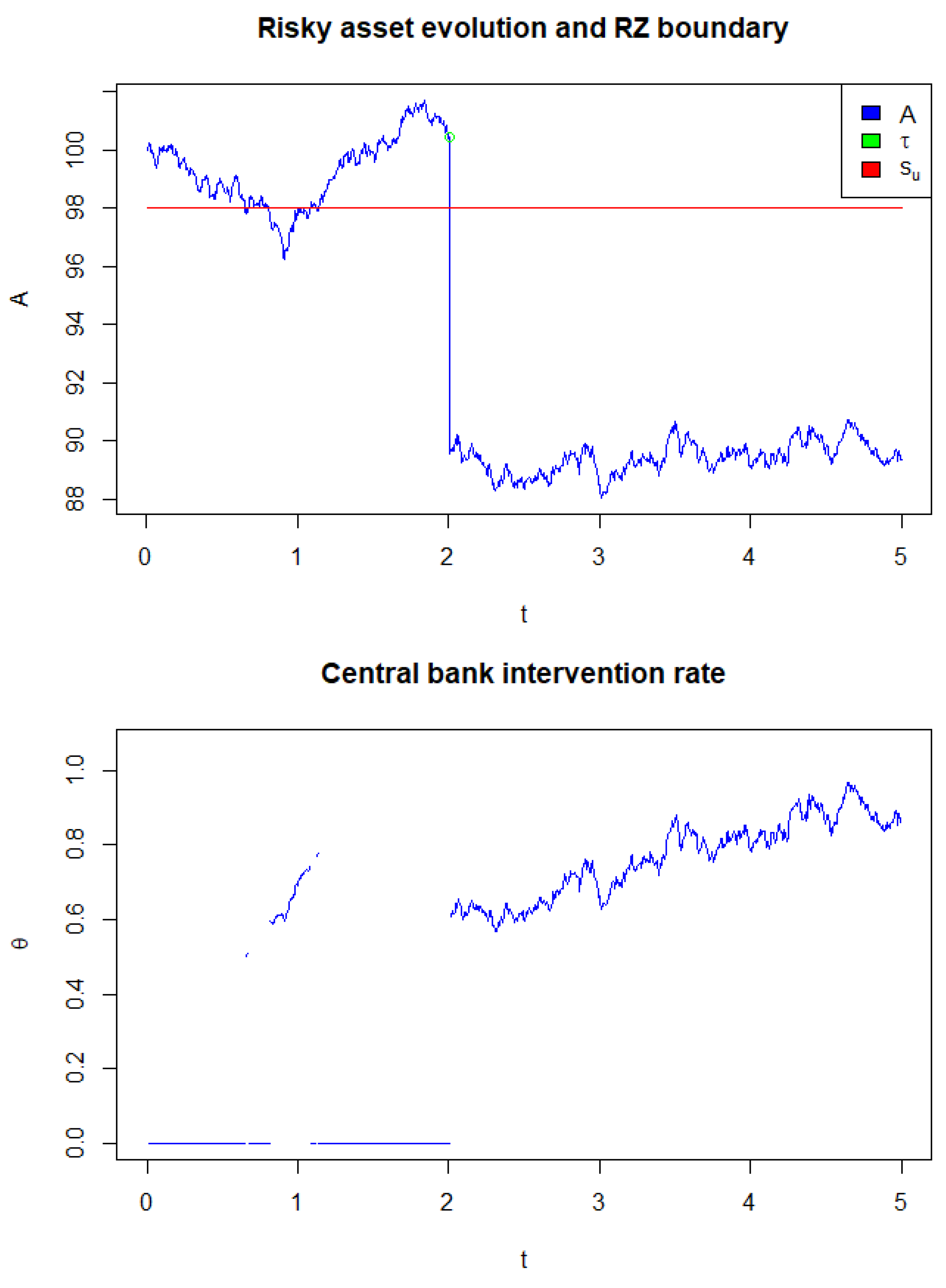
1) and also set that, if the reserve level drops by more than 20% from the current level, the bank is in a very critical economic condition. This means that, at the starting time, the bank is already in a stressed condition. Of course, other assumptions can be considered but, for the purpose of seeing possible multiple government interventions in the next five years, we chose this starting point. If the bank reserves drop by just 2%, the bank is in the “red region”, meaning that the government has the possibility to inject capital in order to contribute to the health of the bank. We also assumed some intensity of the negative jumps that may potentially bring the bank close to collapse despite being very liquid. This situation is similar to what can be seen during the great financial crisis, when some banks were assumed to be very liquid but, after a dramatic drop in their equity value, they were close to bankruptcy. Here, we do not consider the intervention event, which would depend on the intervention rate, in order to see the “natural” evolution of the processes
A and
.
The HJB equation after the introduction of the multiple injection feature becomes
where
is given by the following expression
Let us also underline that, when
,
becomes 0 and the last term in (
27) disappears.
Uniqueness of the Solution
It is worth noting that the arguments in the min-operator in (
28) for
can be split into two parts
The jump part corresponding to the government intervention, that is
We will focus on the component corresponding to the multiple injection of the government intervention, that is, Equation (
30).
The main result of this section is to show that (
26) is the unique viscosity solution of (
28). To prove it, we consider the following standard assumptions on the regularity of
and
:
is measurable on its domain;
There exists a constant dominating on its whole domain, i.e., ;
is measurable, and all ;
is a probability measure on .
see (
Bandini and Confortola 2017, Hyp. 2.1) for further details. Notice that
satisfies the above assumptions. As a result, we consider a setting similar to the one presented in
Bandini and Confortola (
2017) and we have the following result:
Corollary 1. Let us assume that the penalization component of the value function, that is , is measurable and bounded. If we further assume (29) to be measurable with respect to its sigma-algebra and bounded and to satisfy a growth condition, see (Bandini and Confortola 2017, Hyp. 2.3), then we have that Equation (28) has a unique solution in the viscosity sense and this solution is given by (26).
Clearly the liquidation payment function
defined in (
4) satisfies the assumption in Corollary 1.


