A Forward-Looking IFRS 9 Methodology, Focussing on the Incorporation of Macroeconomic and Macroprudential Information into Expected Credit Loss Calculation

Abstract

The International Financial Reporting Standard (IFRS) 9 relates to the recognition of an entity’s financial asset/liability in its financial statement, and includes an expected credit loss (ECL) framework for recognising impairment. The quantification of ECL is often broken down into its three components, namely, the probability of default (PD), loss given default (LGD), and exposure at default (EAD). The IFRS 9 standard requires that the ECL model accommodates the influence of the current and the forecasted macroeconomic conditions on credit loss. This enables a determination of forward-looking estimates on impairments. This paper proposes a methodology based on principal component regression (PCR) to adjust IFRS 9 PD term structures for macroeconomic forecasts. We propose that a credit risk index (CRI) is derived from historic defaults to approximate the default behaviour of the portfolio. PCR is used to model the CRI with the macroeconomic variables as the set of explanatory variables. A novice all-subset variable selection is proposed, incorporating business decisions. We demonstrate the method’s advantages on a real-world banking data set, and compare it to several other techniques. The proposed methodology is on portfolio-level with the recommendation to derive a macroeconomic scalar for each different risk segment of the portfolio. The proposed scalar is intended to adjust loan-level PDs for forward-looking information.

1. Introduction

During the financial crisis, the International Accounting Standard Board (IASB) and Financial Accounting Standard Board (FASB) joined their efforts to redesign accounting standards for an improved and simplified expected credit loss (ECL) framework, and released the International Financial Reporting Standard (IFRS) 9 in 2014 (IFRS 2014). It is common in risk management practices to split the calculation of credit losses into three components: the probability of default (PD), loss given default (LGD), and exposure at default (EAD). A simplified expression for calculating expected credit loss is $ECL=PD\times LGD\times EAD$. When using a PD term structure (marginal PDs), the expression changes as follows to calculate the ECL at account level:

$$EC{L}_i={{\displaystyle \sum }}_{t=1}^T{p}_{i,t}^m\times l_{i,t}\times e_{i,t},$$

(1)

where $p_{i,t}^m$ is the marginal PD, $l_{i,t}$ is the LGD when an account defaults at time $t$, and $e_{i,t}$ the EAD at time $t$, for account $i$ (see for e.g., (Breed et al. 2021) and (Schutte et al. 2020)).

The IFRS 9 standard (IFRS 2014) requires that the PD model accommodates the influence of the current and the forecasted macroeconomic conditions on default rates, enabling forward-looking estimates on impairments. This paper proposes a methodology for adjusting IFRS 9 PD term structures for macroeconomic forecasts in estimating IFRS 9 forward-looking losses. This paper assumes the existence of a PD term structure for IFRS 9 and will focus only on how to adjust the term structure for macroeconomic conditions. To read more about possible PD term structure methodologies for IFRS 9, see Breed et al. (2021) and Schutte et al. (2020).

IFRS 9, being a principle-based accounting standard. According to the Global Public Policy Committee (GPPC) (2016), IFRS 9 does not prescribe specific methodologies for adjusting PDs for macroeconomic conditions, and no single methodology is suitable for all portfolios. The literature on IFRS 9 specific PD methodologies and the incorporation of macroeconomic adjustments is scarce. Several possible ways of incorporating macroeconomic conditions in credit risk modelling are summarised in (Tasche 2013) and (Crook and Bellotti 2010). Several of these may be applied in the IFRS 9 context. In this paper, we consider a scalar approach. Therefore, the ECL in Equation (1) can be adjusted for forward-looking macroeconomic conditions by applying a scalar to each of the ECL components:

$$EC{L}_i^F={{\displaystyle \sum }}_{t=1}^T{p}_{i,t}^m\times s_t^p\times l_{i,t}\times s_t^l\times e_{i,t}\times s_t^e,$$

(2)

where $s_t^p$, $s_t^l$, and $s_t^e$ are the macroeconomic scalars at time $t$ for PD, LGD, and EAD, respectively. The scope of this paper will focus on the PD scalar.

We will use principal component regression (PCR) to derive a macroeconomic scalar. Principal component regression (PCR) is a regression analysis technique based on principal component analysis (PCA). Specifically, PCR is used to estimate the unknown regression coefficients in a standard linear regression model (Jolliffe 1982). Our research contribution is threefold: We will first establish a link between historic macroeconomic conditions and the corresponding impact on the default behaviour of the portfolio, called the credit risk index (CRI). Secondly, we propose a specific variable selection method in the IFRS 9 context. Thirdly, PCR is used to model the CRI with the macroeconomic variables as the set of explanatory variables. Note that, when we refer to macroeconomic variables, we include both the macroeconomic and macroprudential variables. The intended application of the CRI model proposed in the article is for it to be used in conjunction with a loan-level PD model, which is based on an appropriate method to predict both 12 month (Stage 1) and lifetime (Stage 2) PDs. The paper is structured as follows: In Section 2 we give a brief literature review. Section 3 describes our proposed methodology. In Section 3.1 we will discuss the derivation of the CRI and adjustment thereof for seasonality and volatility. Section 3.2 discusses the selection of the macroeconomic variables using PCA and the link to the CRI. Finally, Section 3.3 will derive the macroeconomic scalar. Section 4 illustrates the proposed PCR methodology described in Section 3 on a secured retail portfolio from one of the major banks in South Africa. Finally, Section 5 concludes the paper and discusses future recommendations.

2. Literature Review

The requirement that the PD model, according to IFRS 9 (IFRS 2014), should accommodate the influence of current and forecasted macroeconomic conditions on default rates, results in forward-looking estimates of impairments.

The work of Crook and Bellotti (2010) examined various classes of modelling techniques that can incorporate macroeconomic information. This work is not in the IFRS 9 context, but could be applied within IFRS 9 models. These classes are broadly categorised into portfolio-level and loan-level models. Under loan-level models, they discuss survival models, panel models, and correction factor models, and under portfolio-level models, they discuss loss distributions, Merton-type models, and econometric models.

Examples in literature where portfolio-level models were used can be found in Durović (2019) and Crook and Bellotti (2010). Bellini (2019) further lists the traditional VAR (vector auto-regression) and VEC (vector error-correction) models as the essential toolkit to deal with macroeconomic time series. Jacobs (2019) also used autoregressive vector modelling, specially VARMAX, which adds exogenous variables into the more traditional VAR models. Tasche (2015) utilises regression models to regress the default rate on macroeconomic variables, but emphasises that this approach has the disadvantage that long time series of observations are required. This disadvantage is true for all classes of modelling techniques that incorporate macroeconomic information. In Simons and Rolwes (2009), many techniques are listed under portfolio-level macroeconomic models, including logistic regression, econometric models, and vector autoregression models. Simons and Rolwes (2009) explored the relationship between the default rate and the macroeconomy by developing a logit model with macroeconomic parameters. This reasonably simple model had the following advantages: the model is straightforward, relatively easy to understand, and has robust results. In addition, portfolio-level models are easier to build because they typically require less data and can be implemented faster (Black 2016).

Several loan-level modelling techniques are listed in Bellini (2019) that can be used to model default, taking into account macroeconomic variables: generalised linear models, survival analysis, and many machine learning techniques (e.g., bagging, boosting, and random forests). However, loan-level models require reliable historical loan-level data (Black 2016), and are more difficult to build (more data), and might be slower to implement than portfolio-level models. The most popular loan-level modelling technique within the credit risk context is the use of proportional hazard models (Bellotti and Crook 2013). The benefits of using a hazard model include that time dummies can be utilised, and the effect of prepayment can be added to the modelling process. The option also exists to add competing risks to the modelling process when loan-level hazard models are used (Fine and Gray 1999).

We will investigate the use of PCR in the context of modelling macroeconomic variables. PCR is a regression analysis technique that is based on PCA. First, a PCA will be performed on all $C$ combinations of variables. PCs are linear combinations of all the variables constructed to be jointly uncorrelated, and to explain the original variables’ total variability, Pearson (1901) and Hotelling (1933). Next, a regression will be fitted on the PCA as variables. We propose using PCR since PCA is a multivariate statistical technique that removes multicollinearity and constructs a new set of independent uncorrelated and orthogonal macroeconomic (systematic) risk factors. Note that generally PCA is used as a dimension reduction technique, but in this paper, we do not use it for dimension reduction. Instead, we use it to ensure no multicollinearity exists and to utilise PCR. The PCR constructs a regression model based on these PCs instead of input variables. This paper will focus on portfolio-level models using PCR as the modelling technique.

3. Methodology

As mentioned in the introduction, the forward-looking adjustment of the ECL is made by multiplying the marginal PD $p_{i,t}^m$ with a macroeconomic scalar $s_t^p$ (for the sake of simplicity, we will drop the superscript $p$). The macroeconomic scalar at time $t$ can be estimated by

$${\widehat{s}}_t=\frac{Predicteddefaultrat{e}_t}{Basedefaultrate},$$

(3)

where the $Base default rate$ is an average default rate over that same period of construction of the marginal PD term structure, and $Predicted default rat{e}_t$ is the predicted default rate at time $t$ using macroeconomic variable forecasts.

A link needs to be established between historic macroeconomic conditions and the corresponding impact on the default behaviour of the portfolio. From historic defaults, the CRI is derived to approximate the default behaviour of the portfolio. Finally, PCR is used to model the CRI with the macroeconomic variables as the set of explanatory variables.

The PCR method is divided into three major steps:

• Perform PCA on the explanatory variables ${\mathit{X}}_{n\times p}={\left({\mathit{x}}_1,\dots ,{\mathit{x}}_{\mathit{n}}\right)}^T$ to obtain the principal components ${\mathit{W}}_{n\times p}={\left({\mathit{w}}_1,\dots ,{\mathit{w}}_n\right)}^T$, where $\mathit{W}=\mathit{V}\mathit{X}$ and ${\mathit{V}}_{p\times p}$ the orthonormal set of eigenvectors. Then, select a subset ${\mathit{W}}_{\kappa }=\mathit{X}{\mathit{V}}_{\kappa }$, with ${\mathit{V}}_{\kappa }=\left({\mathit{v}}_1,\dots ,{\mathit{v}}_{\kappa }\right)$, where $\kappa =\min \left\{\kappa :{{\displaystyle \sum }}_{j=1}^{\kappa }{\lambda }_j/{{\displaystyle \sum }}_{j=1}^p{\lambda }_j\ge \delta \right\};\delta \approx 1$ and ${\lambda }_j$ the $j$th eigenvalue of ${\mathit{X}}^T\mathit{X}$.
• Regress the observed vector ${\mathit{Y}}_{n\times 1}={\left(y_1,\dots ,y_n\right)}^T$ of outcomes on the selected principal components as covariates, $\mathit{Y}={\mathit{W}}_{\kappa }{\mathit{\gamma }}_{\kappa }+\mathit{ϵ}$, using ordinary least squares regression to obtain a vector of estimated regression coefficients, ${\widehat{\mathit{\gamma }}}_{\kappa }$, with dimension equal to the number of selected principal components $\kappa .$
• Transform the vector ${\widehat{\mathit{\gamma }}}_{\kappa }$ back to the scale of the actual covariates ${\widehat{\mathit{\beta }}}_{\mathit{\kappa }}={\mathit{V}}_{\kappa }{\widehat{\mathit{\gamma }}}_{\kappa }$, using the selected PCA loadings (the eigenvectors corresponding to the selected principal components) to obtain the final PCR estimator ${\widehat{\mathit{\beta }}}_{\kappa }$ (with dimension equal to the total number of covariates) for estimating the regression coefficients characterising the original model.

The benefits of using the PCR model are that no multicollinearity exists and that the coefficients of the macroeconomic variables in a PCR model are more balanced, i.e., the influence of variables is more evenly distributed amongst the majority of the variables such that no large weight is placed on any single variable. We would prefer that a single macroeconomic variable does not dominate the model by having a very high coefficient relative to the other variables. The benefits of the proposed selection criteria are to ensure: the intuitiveness of the signs and relationships between input variables and target are enforced; the optimal lags of each macroeconomic variables are selected; a larger subset of variables is used in the model, and as such, it is more likely to obtain a model that does not strongly rely on only one or two variables.

In Section 3.1, we will discuss the derivation of the CRI and adjustment thereof for seasonality and volatility. Section 3.2 discusses the selection of the macroeconomic variable using PCA and the link to the CRI. Finally, Section 3.3 contains the derivation of the macroeconomic scalar.

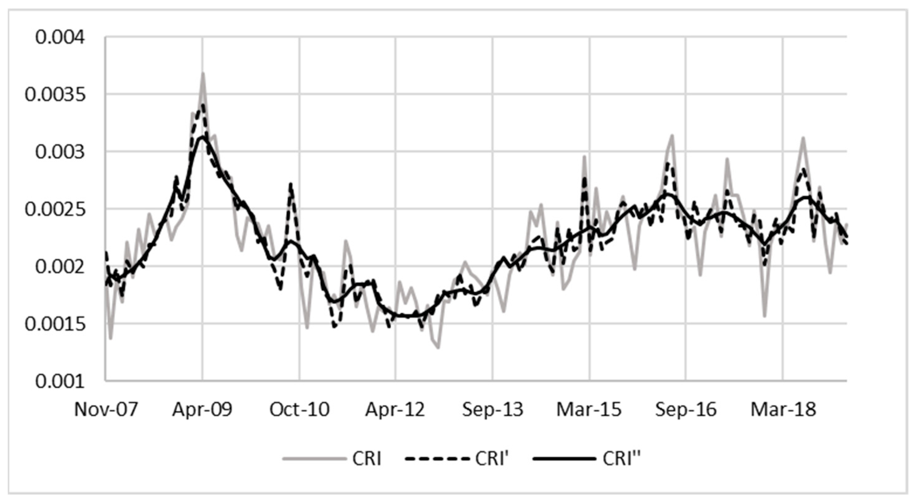
3.1. Credit Risk Index

The CRI, which approximates the default behaviour of the portfolio, is defined as the average marginal default rate with respect to a specific reference month. The concept of a CRI is not new and will typically be derived from historic defaults to approximate the default behaviour of the portfolio (Engelmann 2021). This credit index should be closely related to the specific portfolio a bank is modelling, e.g., country-wide default rates (Engelmann 2021). The vital criterion for such a CRI is the existence of a macroeconomic model that allows the estimation of an abstract state of the economy that imitates the macroeconomic conditions of a bank’s portfolio (Engelmann 2021). We propose a specific way to adapt the historical default rate to carefully capture the link between default behaviour and the macroeconomic environment. To define the CRI, let us consider the following notation, where $\left\{O_1,O_2,\dots ,O_N\right\}$ is the set of observation months e.g., {201509, 201510, …, 201609}. $d_{n,t}$ is the number of accounts that were performing as at the observation month $O_n$, and then defaulted in the period $\left(t-1,t\right]$ months after the observation month, and $a_n$ is the number of performing accounts as at the observation month $O_n$.

Table 1. Illustrative example of marginal defaults.

Observation Date $\mathbf{\left(}{\mathit{O}}_{\mathit{n}}\mathbf{\right)}$	Performing Accounts $\mathbf{\left(}{\mathit{a}}_{\mathit{n}}\mathbf{\right)}$	Months after Observation (t)
		1	2	3	4	5	6	7	8	9	10	11	12
201509	1167	4	7	12	41	45	40	34	41	32	36	35	35
201510	1180	4	7	10	46	42	35	44	36	40	38	37	40
201511	1208	4	7	20	45	38	45	38	43	40	42	42	40
201512	1221	3	13	18	40	48	38	43	44	43	44	43	34
201601	1220	7	10	13	49	39	41	42	43	44	44	34	36
201602	1251	5	8	19	40	44	42	45	47	48	38	38	51
201603	1295	4	13	14	47	48	48	52	53	43	44	58	49
201604	1311	7	10	15	49	49	48	53	44	46	59	51	60
201605	1329	6	11	13	52	54	51	45	49	63	54	63	69
201606	1367	6	9	9	56	55	46	52	66	57	67	74	59
201607	1421	6	7	9	58	54	59	76	65	76	85	69	67
201608	1461	4	6	8	57	64	79	69	81	93	73	74	64

presents the data for $d_{n,t}$ and $a_n$ for observation months {201509, 201510, …, 201609}.

To illustrate the calculation of the CRI, let us consider the data in Table 1. To calculate the CRI for 201609

$$CR{I}_{201609}=\left(\frac{4}{1461}+\frac{7}{1421}+\cdots +\frac{35}{1167}\right)/12.$$

(4)

Thus, the CRI for observation month 201609 is calculated as the average monthly marginal default rate, with respect to 201609 as the reference month, i.e., the highlighted cells in Table 1 are the monthly marginal default rates for 201609 as a reference concerning the previous 12 observation months.

Some motivation regarding our choice of the use of 12 months in Equation (4):

• Limiting the CRI to the observation that was observed in the last 12 months ensures having the same “horizons” for all observation months. If it is not limited to the last 12 months, some months will have a different number of observation months, and the denominator will not be equal over time.
• Using 12 months ensures that the changes in macroeconomic conditions are reflected in more recent populations and not confused with the behaviour far in the past (i.e., more than 12 months ago).
• The CRIs included in the development data are based only on up-to-date accounts. This is due to the assumption that an increase in credit risk has already impacted accounts that have missed at least one payment, and the behaviour of these accounts is thus more likely to be driven by a deteriorated probability of default than a deteriorated economic outlook. In addition, these up-to-date accounts have an expected lifetime of 12 months according to IFRS 9 principles (i.e., Stage 1), which serve as further motivation for specifically using a 12-month outcome period in the CRI calculation.

More generally, the CRI for observation month $n$ is defined as

$$CR{I}_n=\frac{{{\displaystyle \sum }}_{t=1}^{12}\frac{d_{n-t,t}}{a_{n-t}}}{12}.$$

(5)

Typically, monthly default rates will be influenced by non-macroeconomic factors impacting the shape of the CRI. Therefore, the following factors will be considered from a business perspective: seasonality and volatility in the CRI. These two factors will be illustrated in the results in Section 4.

Controlling the effect of seasonality and volatility will ensure that an appropriate CRI is used for modelling purposes that are not distorted by idiosyncratic effects.

Seasonality: Intra-year seasonality effects (e.g., higher default rates post the festive season/Easter break) are typical in default behaviour. The seasonality effects are reduced by adjusting the CRI, as follows

$$CR{I}_n^{\prime }=CR{I}_n+\left(\overline{CRI}-{\overline{CRI}}^h\right),$$

(6)

where $CR{I}_n$ is observation month $n$, $\overline{CRI}$ is the average CRI over the entire development history, ${\overline{CRI}}^h$ is the average CRI for a respective calendar month (i.e., $h=January, February,\dots ,December$), over the entire development history, and $h$ equal to the calendar month of the observation month. Therefore, each monthly CRI is shifted up or down based on how far the average CRI for the respective calendar month deviates from the overall average CRI for the entire sample.

Volatility: The second non-macroeconomic effect to control is volatility, which may be achieved by smoothing the CRI. LOESS (locally estimated scatterplot smoothing) regression is considered for the smoothing technique. With LOESS regression (Cleveland 1979), multiple non-parametric regression type models are combined in a k-nearest-neighbour model, i.e., each output observation from the LOESS regression is a combination (often weighted) of its k-nearest-neighbours (Cleveland 1981). It is a generalisation of a moving average/polynomial regression. It has the advantage that it often does well over the classic smoothing procedures. It does not require the user to specify the function class (i.e., it is non-parametric). We denote $CR{I}_n^{″}$ as the smoothed $CR{I}^{\prime }$ for observation month $n$.

It is important to capture the portfolio’s inherent default behaviour without business decisions to link to macroeconomic conditions.

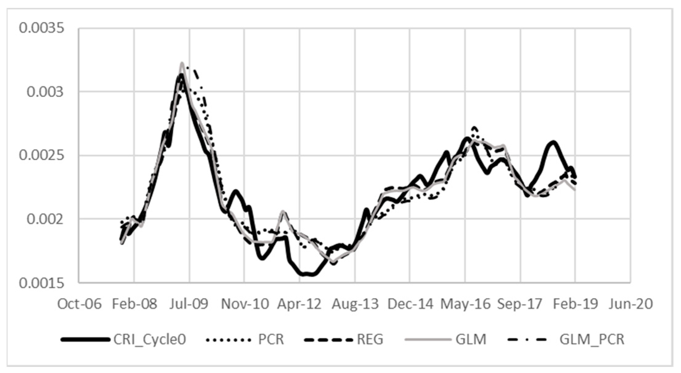
3.2. Principal Component Regression

Numerous possible macroeconomic variables may be used in the modelling process (refer to Section 2 for references). Several considerations should be taken into account when selecting the macroeconomic variables, for example, the reliability and availability of data. Another important aspect is the availability of forecasts for these variables. These forecasts usually consist of a baseline, upturn, and downturn scenario, for example, the forecast provided by Moody’s (PWC 2017). Lastly, input from business stakeholders should be taken into account.

Let ${\mathit{M}}_n=\left\{M_{n,1},M_{n,2},\dots M_{n,P}\right\}$ at observation month $n$ be the set of macroeconomic variables that were identified given the consideration above. Given the possible different scales of macroeconomic variables, we standardise the variables as ${\mathit{Z}}_n=\left\{Z_{n,1},Z_{t,2},\dots Z_{n,P}\right\}$, where $Z_{n,p}=\frac{M_{n,p}-{\overline{M}}_p}{{\sigma }_p}$, where $Z_{n,p}$ is the $p$-th standardised macroeconomic variable at observation month $n$ with ${\overline{M}}_p$, and ${\sigma }_p$, the mean and standard deviation, respectively.

When considering the macroeconomic variables, one should also consider the lags in these variables. Typical lags to be considered are 3, 6, 9, and 12 months, but the business should decide on the final set of lags. Now define the set of standardised lagged macroeconomic variables at observation month $n$ as ${\mathit{Z}}_{n,l}=\left\{Z_{n-l,1},Z_{n-l,2},\dots Z_{n-l,P}\right\}$, where $l$ indicates the lag, for example, $l=\left\{0, 3, 6, 9, 12\right\}$ (Note ${\mathit{Z}}_{n,0}=$ ${\mathit{Z}}_n$).

All possible combinations of variables will be considered, with a minimum of 3 variables in a combination, and a maximum of $P^{\prime }\le P$. These combinations will also include all lags but will be restricted not to include both a variable and its lag in the same combination. The reason for this requirement is to ensure that a single variable does not dominate the model (by appearing more than once in the model), and this requirement also decreases the chance of multicollinearity (typically, lags of variables are highly correlated). Let $I^c$ be the set of all these possible combinations ranging from size 3 to $P^{\prime }$, with $c=1,\dots ,C$ the number of combinations. $C$ can be calculated as $C={{\displaystyle \sum }}_{i=3}^{P^{\prime }}\left(\begin{array}{c}P\\ i\end{array}\right)\times L^i$ where $L$ is the number of lags considered. Then, let ${\mathit{Z}}_n^c$ be the vector with elements ${\left\{Z_{n-l,i}\right\}}_{i\in I^c}$. In the PCR, the set of exploratory variables $\mathit{X}={\left({\mathit{x}}_1,\dots ,{\mathit{x}}_n\right)}^T$ are therefore ${\mathit{x}}_n={\left({\mathit{Z}}_n^c\right)}^T$, i.e., $\mathit{X}={\mathit{Z}}^c={\left({\mathit{Z}}_1^c,\dots ,{\mathit{Z}}_n^c\right)}^T$.

As an example, assume there are three macroeconomic variables, $Z_{n-l,1},Z_{n-l,2}{Z}_{n-l,3}$, and lags 0, 3, and 6 are considered. Then, the $C=27$ combinations considered are given in

Table 2. Illustrative example of combinations sets.

$\left(Z_{n,1},Z_{n,2}{Z}_{n,3}\right)$	$\left(Z_{n,1},Z_{n,2}{Z}_{n-3,3}\right)$	$\left(Z_{n,1},Z_{n,2}{Z}_{n-6,3}\right)$
$\left(Z_{n-3,1},Z_{n,2}{Z}_{n,3}\right)$	$\left(Z_{n-3,1},Z_{n,2}{Z}_{n-3,3}\right)$	$\left(Z_{n-3,1},Z_{n,2}{Z}_{n-6,3}\right)$
$\left(Z_{n-6,1},Z_{n,2}{Z}_{n,3}\right)$	$\left(Z_{n-6,1},Z_{n,2}{Z}_{n-3,3}\right)$	$\left(Z_{n-6,1},Z_{n,2}{Z}_{n-6,3}\right)$
$\left(Z_{n,1},Z_{n-3,2}{Z}_{n,3}\right)$	$\left(Z_{n,1},Z_{n-3,2}{Z}_{n-3,3}\right)$	$\left(Z_{n,1},Z_{n-3,2}{Z}_{n-6,3}\right)$
$\left(Z_{n-3,1},Z_{n-3,2}{Z}_{n,3}\right)$	$\left(Z_{n-3,1},Z_{n-3,2}{Z}_{n-3,3}\right)$	$\left(Z_{n-3,1},Z_{n-3,2}{Z}_{n-6,3}\right)$
$\left(Z_{n-6,1},Z_{n-3,2}{Z}_{n,3}\right)$	$\left(Z_{n-6,1},Z_{n-3,2}{Z}_{n-3,3}\right)$	$\left(Z_{n-6,1},Z_{n-3,2}{Z}_{n-6,3}\right)$
$\left(Z_{n,1},Z_{n-6,2}{Z}_{n,3}\right)$	$\left(Z_{n,1},Z_{n-6,2}{Z}_{n-3,3}\right)$	$\left(Z_{n,1},Z_{n-6,2}{Z}_{n-6,3}\right)$
$\left(Z_{n-3,1},Z_{n-6,2}{Z}_{n,3}\right)$	$\left(Z_{n-3,1},Z_{n-6,2}{Z}_{n-3,3}\right)$	$\left(Z_{n-3,1},Z_{n-6,2}{Z}_{n-6,3}\right)$
$\left(Z_{n-6,1},Z_{n-6,2}{Z}_{n,3}\right)$	$\left(Z_{n-6,1},Z_{n-6,2}{Z}_{n-3,3}\right)$	$\left(Z_{n-6,1},Z_{n-6,2}{Z}_{n-6,3}\right)$

below:

The PCR is fitted to all the possible combinations of macroeconomic variables sets ${\mathit{Z}}^c$ with $CR{I}_n^{\prime }$ as the target variable. Out of all the fitted models, we selected only the models that fulfil the following criteria:

• The estimated sign for the regression coefficients ${\widehat{\mathit{\beta }}}_{\kappa }^c$ of the macroeconomic variables should be in line with economic expectations. For example, the estimated sign for the GDP coefficient should be negative since we expect default rates to decrease when GDP increases (see Durović 2019).
• All estimated coefficients of ${\widehat{\mathit{\gamma }}}_{\kappa }^c$ are statistically significant at $\alpha \%$ significance level, for example, $\alpha =0.05$ (see Durović 2019).

The remaining models can be ranked using some measure of model fit, for example, $R$-square, AIC (Akaike’s information criterion), AICC (corrected AIC), BIC (Sawa Bayesian information criterion), or the RMSE (root mean square error). In our case study below, we used the AICC. The AICC, therefore, is used to determine the ‘optimal’ variable combination. The best model, $c^{\prime }$, can then be selected, taking into account other business considerations.

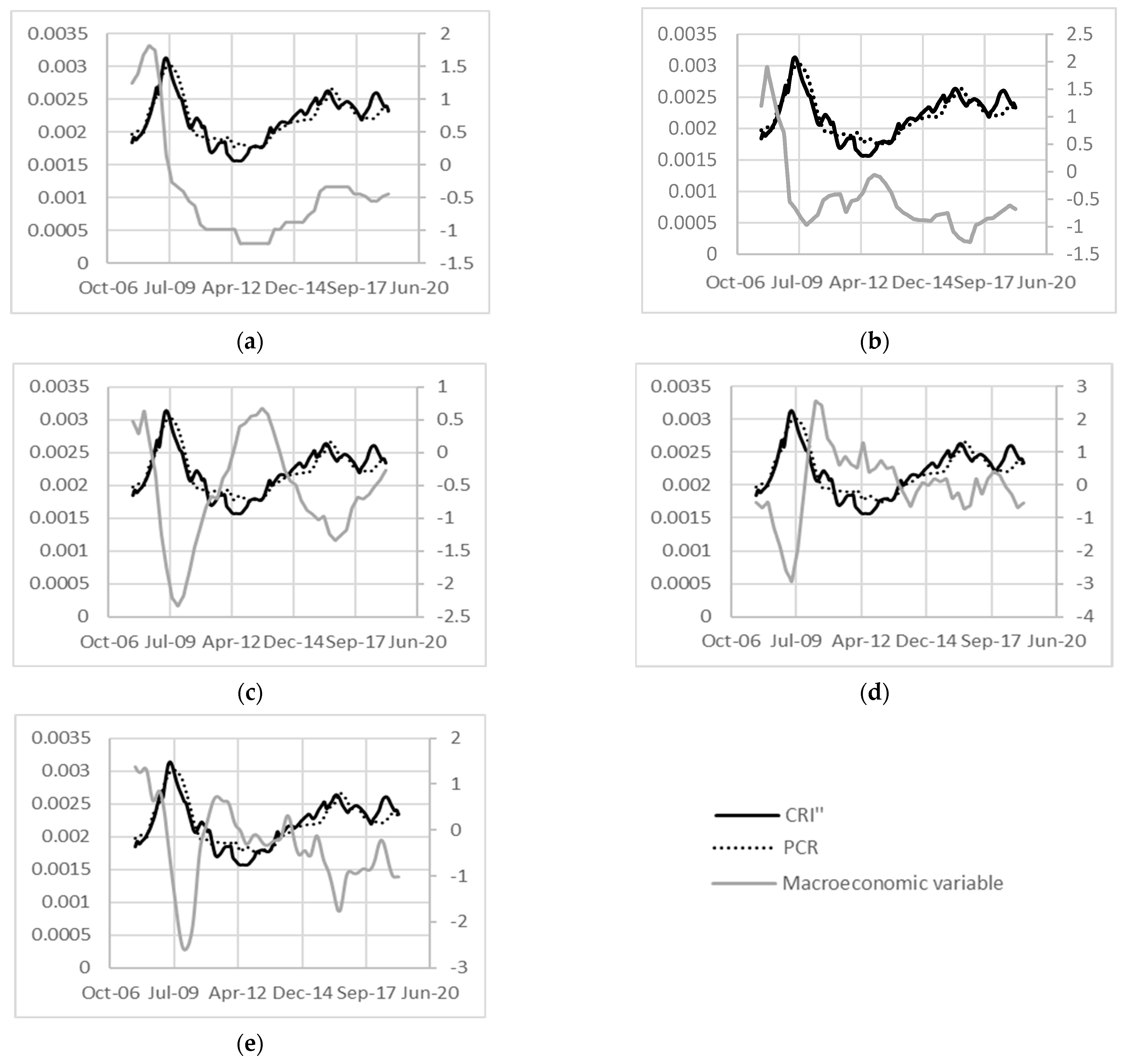
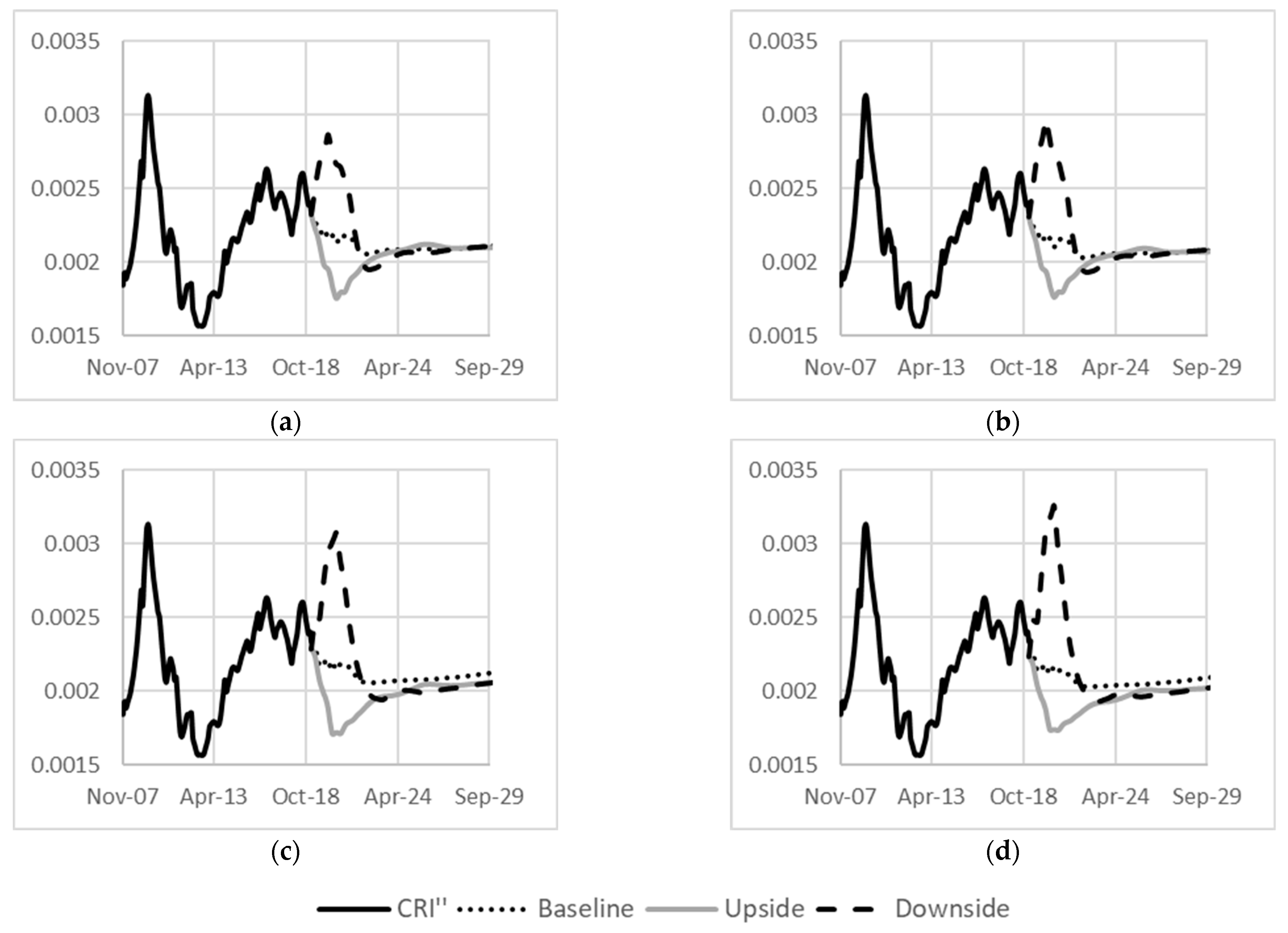
3.3. Derivation of the Macroeconomic Scalar

Let ${\mathit{M}}_t^{c^{\prime },g}$ be the forecasts for time $t$ of the macroeconomic variables selected in the final model $c^{\prime }$. Several forward-looking macroeconomic scenarios $g$ can be considered, for example, a baseline, upside, and downside scenario, along with scenario weightings. The number of scenarios used may be based on several factors, for example, PWC (2017). The scenario weightings are determined by both statistical analysis and expert credit judgment, taking into account the range of possible outcomes each selected scenario represents.

Given macroeconomic scenario $g$, the macroeconomic scalar for time $t$ from Equation (3) can be written as

$${\widehat{s}}_t^g=\frac{{\widehat{CRI}}_t^g}{CR{I}_{base}},$$

(7)

where the base default rate, $CR{I}_{base}$, is the weighted average modelled CRI over the period, $O^{\prime }\subset \left\{O_1,O_2,\dots ,O_N\right\}$, aligned to the development period of the PD term structure and calculated as

$$CR{I}_{base}=\frac{{{\displaystyle \sum }}_{n\in O^{\prime }}^{}CR{I}_n^{″}\times w_n}{{{\displaystyle \sum }}_{n\in O^{\prime }}^{}{w}_n},$$

(8)

with weights $w_n$ determined by business considerations. ${\widehat{CRI}}_t^g$ is the forecasted CRI using the macroeconomic forecasts ${\mathit{M}}_t^{c^{\prime },g}$

$${\widehat{CRI}}_t^g={\widehat{\mathit{\beta }}}_{\kappa }^{c^{\prime }}{\mathit{Z}}_t^{c^{\prime },g},$$

(9)

where ${\widehat{\mathit{\beta }}}_{\kappa }^{c^{\prime }}$ the estimated regression coefficients for the selected model $c^{\prime }$ and ${\mathit{Z}}_t^{c^{\prime },g}$, the standardised macroeconomic forecasts for time $t$ and scenario $g$.

Note that the weights in (8) are optional and could also be omitted from Equation (8). There are many ways to determine the weights. Some banks might decide to give lower weights in an extremely volatile economic time-period (such as the Covid pandemic). In this example, outcome months that contributed more to the calculation of CRI received higher weights.

It is possible to segment a portfolio into distinct risk groups (Schutte et al. 2020), and then a macroeconomic scalar can be derived for each different segment. This extension can be researched further, and is listed in Section 5 as a future recommendation.

4. Case Study

This section illustrates the proposed PCR methodology described in Section 3 on a secured retail portfolio from one of the major banks in South Africa. Limited information will be provided due to the data’s confidential nature, and the case study aims to show how our proposed methodology can be implemented. The results were altered (CRI values multiplied by a random value) for confidentiality. In Section 4.1, the data used will be discussed, including the CRI, and adjustments and macroeconomic variables used. In Section 4.2, we will discuss the PCR results and benchmark them against other methods. The resulting macroeconomic scalar will be presented in Section 4.3. We conclude the case study with a section on practical considerations.

4.1. Data

The dataset contains the constructed CRI over the period of November 2007 to February 2019 for up-to-date customers. We typically would like to use a time-span that includes at least a full economic cycle when attempting to model the macroeconomic effect in a portfolio (Crook and Bellotti 2010). The rationale behind using up-to-date customers for development is that macroeconomic factors impact the probability of these customers more intuitively, as customers who are already in arrears (Stage 2 and 3) at observation have already experienced a loss event, and the impact of future-looking information is found to be less significant on their behaviour.

We also have macroeconomic variables over the same period, as well as forecasts for a baseline, upside, and downside scenario over the period March 2019 to December 2048. In total, 13 macroeconomic variables were considered for which forecasts were available:

• Real gross domestic product (GDP);
• Nominal gross domestic product (NGDP);
• Consumer price index (CPI);
• House price index (HPI);
• Prime rate (PR);
• Total disposable household income (DHI);
• Household debt to disposable income (HDDI);
• Debt Service Ratio (DSR);
• New vehicle sales (NVS);
• Credit extended to households (CEH);
• Monetary credit extended (MCE);
• Instalment debtors (ID);
• Overdrafts and loans (OL).

Of these 13, NGDP, HDDI, MCE, and OL were not used due to business decisions and univariate analysis with the target variable. To ensure stationarity, some macroeconomic variables were transformed into year-on-year growth rates.

From Figure 1, seasonality effects are evident in the historical behaviour of the CRI, which are especially prevalent from 2013 onwards, where the CRI is typically higher when observed during May, June, or July. The seasonally adjusted CRI curve ($CR{I}^{\prime }$) in Figure 1 shows the reduction in the increased CRI levels for the seasonal periods. Note, however, that, while some of the observed volatility is reduced because of the seasonality adjustments, high levels of volatility in $CR{I}^{\prime }$ are still observed.

The smoothing of volatility is achieved through LOESS regression. The smoothing parameter used by this approach is a number between 0 and 1, and can be interpreted as the proportion of data used to smooth a region. A low smoothing parameter leads to a smoothed curve that closely follows the input curve (with a value of 0 resulting in the input curve), while a high parameter will lead to a flatter and more smoothed curve (with a value of 1 leading to a flat curve). The optimal (rounded to the second decimal) smoothing parameter was chosen to minimise the AICC criteria (SAS Institute 2013). The optimal smoothing parameter (0.05) provided a good balance between retaining the severity levels of the peaks and troughs, while also minimising the volatility without removing the true underlying trend from the data, as seen in Figure 1 for $CR{I}^{″}$.

4.2. PCR

As mentioned above, we consider nine ($P=9$) macroeconomic variables and used lags 0, 3, and 6. ($L=3$) due to business reasons. We have considered all combinations with a minimum of three variables and a maximum of seven ($P^{\prime }=7$). Given the formula $C={{\displaystyle \sum }}_{i=3}^{P^{\prime }}\left(\begin{array}{c}P\\ i\end{array}\right)\times L^i$, we have a total number of 183060 combinations. When selecting the number of PCs in the PCR, we used at least two PCs, i.e., $\kappa =\max \left(2,\min \left\{\kappa :{{\displaystyle \sum }}_{j=1}^{\kappa }{\lambda }_j/{{\displaystyle \sum }}_{j=1}^p{\lambda }_j\ge \delta \right\};\delta \approx 1\right)$. All macroeconomic variables were standardised.

The PCR was fitted to all the possible combinations of macroeconomic variables, with $CR{I}^{″}$ as the target variable. As discussed in Section 3.2, out of all the fitted models, we only consider the models where the estimated signs for the regression coefficients (${\widehat{\mathit{\beta }}}_{\kappa }^c$) of the macroeconomic variables are in line with economic expectations, and all the estimated PCR coefficients (${\widehat{\mathit{\gamma }}}_{\kappa }^c$) are statistically significant at 5%.

Table 3. Expected regression coefficient (${\widehat{\mathit{\beta }}}_{\kappa }^c$) signs.

Variable Name	Expected Sign
Real gross domestic product (GDP)	Negative
New vehicle sales (NVS)	Negative
Total disposable household income (DHI)	Negative
Consumer price index (CPI)	Positive
Debt Service Ratio (DSR)	Positive
Prime rate (PR)	Positive
Instalment debtors (ID)	Negative
House price index (HPI)	Negative
Credit extended to households (CEH)	Negative

presents the expected signs as provided by the business. The remaining models were ranked using AICC.

Table 4. Top three PCR models ranked by AICC.

Description	Model 1	Model 2	Model 3
Combination number	32680	3819	32483
PC used	2	2	2
AIC	−1914.20	−1910.28	−1909.75
AICC	−1913.89	−1909.98	−1909.44
BIC	−1902.55	−1898.63	−1898.10
RMSE	0.000206	0.000209	0.000210
Number of variables	5	4	5
Variable 1	NVS	NVS	NVS
Variable 2	PR	PR	PR_L3
Variable 3	CEH	CEH	CEH
Variable 4	ID	ID_L3	ID
Variable 5	GDP_L6		GDP_L6
Intercept	0.00208	0.00205	0.00208
Coefficient of variable 1	−0.00022	−0.00028	−0.00020
Coefficient of variable 2	0.00017	0.00019	0.00019
Coefficient of variable 3	−0.00009	−0.00021	−0.00009
Coefficient of variable 4	−0.00026	−0.00036	−0.00025
Coefficient of variable 5	−0.00018		−0.00017

below gives the results from the top three PCR models ranked by AICC. Note that the coefficient values are the resulting regression coefficients (${\widehat{\mathit{\beta }}}_{\kappa }^c$) calculated from the PCA loading (${\mathit{V}}_{\kappa }^c$) and PCR coefficients (${\widehat{\mathit{\gamma }}}_{\kappa }^c$). It is noted that the AICCs of the top three models are close. The variable combinations are similar between the three models deferring only in lags and number of variables.

For PCR Model 32680 (the best PCR model), the PC loadings (${\mathit{V}}_{\kappa }^c$) for PC1 and PC2 were −0.0001 and −0.0004, respectively. The PCR coefficients (${\widehat{\mathit{\gamma }}}_{\kappa }^c$) are depicted in

Table 5. Model 32680 PCR coefficients.

Description	PCA1	PCA2
Coefficient of NVS	−0.24520	0.60779
Coefficient of PR	0.41841	−0.54217
Coefficient of CEH	0.57044	0.03736
Coefficient of ID	0.40922	0.50460
Coefficient of GDP_L6	0.52148	0.28396

, indicating the effect of the principal components of the regression coefficients (${\widehat{\mathit{\beta }}}_{\kappa }^c$).

Our proposed methodology (PCR) was compared to other traditional modelling techniques. We have considered regression (REG), generalised linear models (GLM), and GLM applied on PCR (GLM-PCR).

For the REG model, we regress the $CR{I}^{″}$ directly against the possible combinations of macroeconomic variables sets ${\mathit{Z}}^c$. In the GLM model, we regress the $CR{I}^{″}$ against the possible combinations of macroeconomic variables sets ${\mathit{Z}}^c$ using logit linked function and the inverses Gaussian distribution. The logit linked function is selected since $CR{I}^{″}$ is a value between 0 and 1. The GLM-PCR model is again our original PCR model, however, as with the logit linked function and the inverses, Gaussian distribution is used.

We employed the same variable selection process over the combination set of 183,060 combinations. As with the PCR, we have checked the estimated signs for the regression coefficients (${\widehat{\mathit{\beta }}}_{\kappa }^c$) for all techniques, and only considered models where the estimated coefficients are statistically significant at 5%. For PCR and GLM-PCR, the estimated PCR coefficients (${\widehat{\mathit{\gamma }}}_{\kappa }^c$) are used, and for REG and GLM, the estimated regression coefficients (${\widehat{\mathit{\beta }}}_{\kappa }^c$) are used.

Table 6. Best model for PCR, GLM-PCR, REG and GLM.

Description	PCR	GLM_PCR	REG	GLM
Combination number	32680	32680	3181	3181
PC used	2	2	NA	NA
RMSE	0.000206	0.000233	0.000188	0.000195
Number of variables	5	5	4	4
Variable 1	NVS	NVS	NVS	NVS
Variable 2	PR	PR	DSR	DSR
Variable 3	CEH	CEH	CEH_L3	CEH_L3
Variable 4	GDP_L6	GDP_L6	GDP_L3	GDP_L3
Variable 5	ID	ID
Intercept	0.00208	−4.08182	0.00182	−4.17746
Coefficient of variable 1	−0.00022	−0.07228	−0.00015	−0.04021
Coefficient of variable 2	0.00017	0.05578	0.00054	0.19122
Coefficient of variable 3	−0.00009	−0.02992	−0.00066	−0.23253
Coefficient of variable 4	−0.00018	−0.06145	−0.00014	−0.03765
Coefficient of variable 5	v0.00026	−0.08667

presents the results from the best model for PCR, GLM-PCR, REG, and GLM ranked according to the root mean squared error (RMSE). Note that the best model based on RMSE is the regression model, with our methodology ranking second. In addition, note that the variable combinations are similar between the four models deferring in lags and number of variables, with three of the variables overlapping. Interestingly, the GLM (GLM-PCR) did not improve the REG (PCR), since we expected that the logit link function would be intuitive, given the target variable is bounded between 0 and 1. We also used the probit link function, which did not improve the results.

Table 6 shows that the REG model performs slightly better than the proposed PCR model. However, the benefit of using the PCR model is also seen in the weights of the estimated coefficients, which are more evenly distributed (no single macroeconomic variable dominates the model).

In Figure 2, we observe the fitted models for PCR, GLM-PCR, REG, and GLM against the $CR{I}^{″}$. The different models follow the $CR{I}^{″}$ closely. Figure 3 below displays the proposed PCR model against the selected macroeconomic variables and $CR{I}^{″}$. As expected with our proposed selection criteria, the intuitiveness of the signs and relationships between the macroeconomic variables and the $CR{I}^{″}$ are clear (positive for PR and negative for NVS, CEH, GDP_L6, and ID).

In Figure 4, we show the forecasted $CR{I}^{″}$ for the PCR, GLM-PCR, REG, and GLM models using the selected macroeconomic variables for baseline, upside and downside scenarios. Short-term, we expect that the forecasted $CR{I}^{″}$ will be higher for the downside than the upside scenario. This is true for all four models. However, in the long-term, we expect the three scenarios to converge (see PWC (2017)) and at least be positive. Figure 4 shows that this is somewhat true for all four models. However, the PCR based model converges better.

4.3. Macroeconomic Scalar

In Figure 5, we show the forecasted macroeconomic scalar (${\widehat{s}}_t^g$) for the PCR, GLM-PCR, REG, and GLM models, using the selected macroeconomic variables for baseline, upside, and downside scenarios. As with the forecasted $CR{I}^{″}$, we expect that the short-term forecasted macroeconomic scalar will be higher for the downside than the upside scenario, and the long-term macroeconomic scalar scenarios should converge. Again, this is somewhat true for all four models, however, the PCR based model converges better.

Furthermore, for the macroeconomic scalars, we expect the upside scenario to be lower than one and the downside scenario to be higher than one over the short-term. In the long-term, we expect the macroeconomic scalar to converge to the long-term economic outlook, as captured in the forecasts of the macroeconomic variables. As seen in Figure 4, the current $CR{I}_{base}$ will be higher than the forecasted long-term $CR{I}^{″}$, and therefore, the long-term macroeconomic scalar will be below one in Figure 5.

Note from Figure 4 and Figure 5 that, in our case study, the term $p_{i,t}^m\times s_t^p$ in Equation (2), i.e., the adjusted PD will remain between 0 and 1. If this is not the case, we propose a manual adjustment to ensure this, for example, capping the PD at 1 or flooring at 0.

5. Conclusions & Future Recommendations

This paper proposed a portfolio-level methodology for adjusting IFRS 9 PD term structures for macroeconomic forecasts to estimate IFRS 9 forward-looking losses. The PD adjusted for forward-looking macroeconomic conditions by applying a scalar to the PD component. To derive this macroeconomic scalar, we used principal component analysis and regression. Note that our methodology is on a portfolio-level, but it is recommended that a macroeconomic scalar is then derived for each different risk segment of the portfolio. The scalar (on portfolio or segment-level) is intended to adjust loan-level PDs for forward-looking information.

Our research contribution was threefold: We first established a link between historic macroeconomic conditions and the corresponding impact on the default behaviour of the portfolio, called the credit risk index. Secondly, we proposed a specific variable selection method in the IFRS 9 context. Thirdly, PCR was used to model the CRI with the macroeconomic variables as the set of explanatory variables.

The benefits of using the PCR model are that no multicollinearity exists, and the coefficients of the macroeconomic variables in a PCR model are more balanced in the sense that no large weight is placed on a single variable. The benefits of the proposed selection criteria are to ensure: the intuitiveness of the signs and relationships between input variables and target are enforced; the optimal lags of each macroeconomic variables are selected; a larger subset of variables is used in the model and, as such, it is more likely to obtain a model that does not strongly rely on only one or two variables.

Note that this paper provides a methodology to incorporate macroeconomic forecasts and assumes that these forecasts are accurate. An area for future research is to measure the accuracy of these forecasts and their impact on ECL.

Note that the methodology is built on the assumption that only macroeconomic and macroprudential variables drive the CRI. A future research idea is to analyse this assumption and investigate alternatives. Some alternatives that might be investigated are the possibility of modelling on loan-level. While some disadvantages of loan-level modelling include that it is more difficult to build, many possible advantages could be listed. This includes the opportunity of including competing risks and, therefore, incorporating the effect of prepayment and attrition into the modelling process. Our proposed methodology adjusts loan-level PDs by using a portfolio or segment-level scalar. A future recommendation could be to directly model loan-level PDs that incorporate the macroeconomic information, e.g., model loan-level PDs by using application, behavioural, and macroeconomic variables simultaneously in a model.

Note that a future research recommendation is to investigate the use of machine learning modelling techniques to incorporate macroeconomic information into IFRS 9 PD models. Note that, in the PD modelling case, there has been a lot of success in the use of machine learning techniques (see e.g., Jiang 2022 and Lessmann et al. 2015), but the use of machine learning in the incorporation of macroeconomic variables has not been well documented. We conducted an initial investigation but struggled to ensure the theoretical relationship between macroeconomic variables and the default rate (when using more complex techniques, e.g., VARMAX and random forests). The forecasts that we substitute in the scalar are provided by the bank’s Group Economics department. Typically, these forecasts are very dependent on the theoretical relationships expected between macroeconomic variables and default rate (e.g., we assume if GDP goes up, defaults will go down). This does not necessarily happen in real life. Sometimes, the actual observed relationship is not as straightforward. When building complex models, it is difficult to ensure that the theoretical relationship expected is ensured in these techniques. A future research idea is to investigate the use of machine learning techniques in macroeconomic modelling, and specific research methods to ensure that the “business sense” is captured. This will ensure that the resulting scalars make business sense. In other words, we would like the scalar to be higher than one if we substitute downside forecasts into the macroeconomic model, and we expect a scalar of less than one if we substitute upside forecasts into the model.

References

1. Bellini, Tiziano. 2019. IFRS 9 and CECL Credit Risk Modelling and Validation: A Practical Guide with Examples Worked in R and SAS, 1st ed. London: Elsevier. [Google Scholar]
2. Bellotti, Tony, and Jonathan Crook. 2013. Forecasting and stress testing credit card default using dynamic models. International Journal of Forecasting 29: 563–74. [Google Scholar] [CrossRef] [Green Version]
3. Black, Barnaby. 2016. Probability-Weighted Outcomes Under A Macroeconomic Approach. Available online: https://www.moodysanalytics.com/webinars-on-demand/2016/probablility-weighted-outcomes-macroeconomic-approach (accessed on 9 January 2023).
4. Breed, Douw Gerbrand, Niel van Jaarsveld, Carsten Gerken, Tanja Verster, and Helgard Raubenheimer. 2021. Development of an Impairment Point in Time Probability of Default Model for Revolving Retail Credit Products: South African Case Study. Risks 9: 208. [Google Scholar] [CrossRef]
5. Cleveland, William S. 1979. Robust Locally Weighted Regression and Smoothing Scatterplots. Journal of the American Statistical Association 74: 829–36. [Google Scholar] [CrossRef]
6. Cleveland, William S. 1981. LOWESS: A program for smoothing scatterplots by robust locally weighted regression. The American Statistician 35: 54. [Google Scholar] [CrossRef]
7. Crook, Jonathan, and Tony Bellotti. 2010. Time varying and dynamic models for default risk in consumer loans. Journal of the Royal Statistical Society: Series A (Statistics in Society) 173: 283–305. [Google Scholar] [CrossRef] [Green Version]
8. Durović, Andrija. 2019. Macroeconomic Approach to Point in Time Probability of Default Modeling—IFRS 9 Challenges. Journal of Central Banking Theory and Practice 1: 209–23. [Google Scholar] [CrossRef] [Green Version]
9. Engelmann, Bernd. 2021. A Simple and Consistent Credit Risk Model for Basel II/III, IFRS 9 and Stress Testing when Loan Data History Is Short. Available online: http://dx.doi.org/10.2139/ssrn.3926176 (accessed on 14 February 2022).
10. Fine, Jason P., and Robert J. Gray. 1999. A Proportional Hazards Model for the Subdistribution of a Competing Risk. Journal of the American Statistical Association 94: 496–509. [Google Scholar] [CrossRef]
11. Global Public Policy Committee (GPPC). 2016. The Implementation of IFRS 9 Impairment Requirements by Banks: Considerations for Those Charged with Governance of Systemically Important Banks. Global Public Policy Committee. Available online: http://www.ey.com/Publication/vwLUAssets/Implementation_of_IFRS_9_impairment_requirements_by_systemically_important_banks/$File/BCM-FIImpair-GPPC-June2016%20int.pdf (accessed on 7 September 2021).
12. Hotelling, Harold. 1933. Analysis of a Complex of Statistical Variables into Principal Components. Journal of Educational Psychology 24: 417–441, 498–520. [Google Scholar] [CrossRef]
13. IFRS. 2014. IRFS9 Financial Instruments: Project Summary. Available online: http://www.ifrs.org/Current-Projects/IASB-Projects/Financial-Instruments-A-Replacement-of-IAS-39-Financial-Instruments-Recognitio/Documents/IFRS-9-Project-Summary-July-2014.pdf (accessed on 31 January 2016).
14. Jacobs, Michael. 2019. An Analysis of the Impact of Modeling Assumptions in the Current Expected Credit Loss (CECL) Framework on the Provisioning for Credit Loss. Journal of Risk & Control 6: 65–112. [Google Scholar]
15. Jiang, Yixiao. 2022. A Primer on Machine Learning Methods for Credit Rating Modeling. In Econometrics-Recent Advances and Applications. London: IntechOpen. [Google Scholar] [CrossRef]
16. Jolliffe, Ian T. 1982. A note on the Use of Principal Components in Regression. Journal of the Royal Statistical Society, Series C 31: 300–3. [Google Scholar] [CrossRef] [Green Version]
17. Lessmann, Stefan, Bart Baesens, Hsin-Vonn Seow, and Lyn Thomas. 2015. Benchmarking state-of-the-art classification algorithms for credit scoring: An update of research. European Journal of Operational Research 247: 124–36. [Google Scholar] [CrossRef] [Green Version]
18. Pearson, Karl. 1901. On Lines and Planes of Closest Fit to Systems of Points in Space. Philosophical Magazine 6: 559–72. [Google Scholar] [CrossRef] [Green Version]
19. PWC. 2017. In Depth IFRS 9 Impairment: How to Include Multiple Forward-Looking Scenarios. London: PWC. [Google Scholar]
20. SAS Institute. 2013. SAS/STAT 13.1 User’s Guide: The LOESS Procedure. Cary: SAS Institute Inc. [Google Scholar]
21. Schutte, Willem Daniel, Tanja Verster, Derek Doody, Helgard Raubenheimer, and Peet Jacobus Coetzee. 2020. A proposed benchmark model using a modularised approach to calculate IFRS9 expected credit loss. Cogent Economics & Finance 8: 1735681. [Google Scholar]
22. Simons, Dietske, and Ferdinand Rolwes. 2009. Macroeconomic Default Modeling and Stress Testing. International Journal of Central Banking 5: 177–204. [Google Scholar]
23. Tasche, Dirk. 2013. The art of probability-of-default curve calibration. Journal of Credit Risk 9: 63–103. [Google Scholar] [CrossRef] [Green Version]
24. Tasche, Dirk. 2015. Forecasting Portfolio Credit Default Rates. Available online: https://www.bayes.city.ac.uk/__data/assets/pdf_file/0015/256101/TASCHE-Dirk-10.02.2015.pdf (accessed on 22 April 2022).
Figure 1. Constructed, seasonality adjusted and LOESS smoothed CRI.
Risks 11 00059 g001
Figure 2. Fitted models for PCR, GLM-PCR, REG, and GLM against C R I .
Risks 11 00059 g002
Figure 3. PCR model against macroeconomic variables and C R I . (a) PR; (b) CEH; (c) ID; (d) NVS; (e) GDP_L6.
Risks 11 00059 g003
Figure 4. Forecasted C R I for PCR, GLM-PCR, REG and GLM with baseline, upside, and downside macroeconomic scenarios. (a) PCR; (b) GLM-PCR; (c) REG; (d) GLM-REG.
Risks 11 00059 g004
Figure 5. Macroeconomic scalar for PCR, GLM-PCR, REG, and GLM with baseline, upside, and downside macroeconomic scenarios. (a) PCR; (b) GLM-PCR; (c) REG; (d) GLM-REG.
Risks 11 00059 g005