

Enhanced Preprocessing Approach Using Ensemble Machine Learning Algorithms for Detecting Liver Disease

Abstract
:1. Introduction
2. Literature Survey
3. Problem Statement
4. Proposed Architecture Using Ensemble Learning with Enhanced Preprocessing
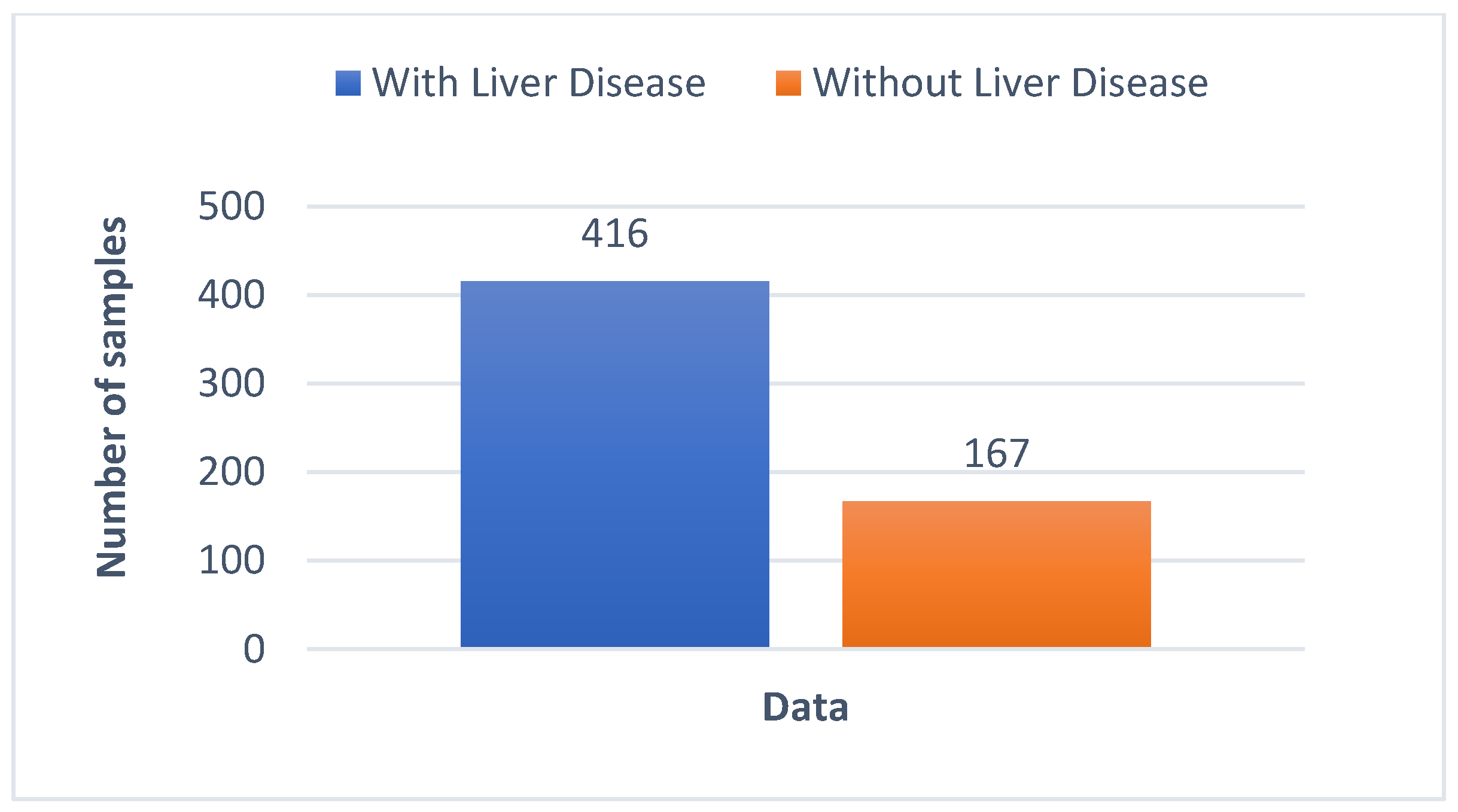
4.1. Dataset to Perform Liver Disease Classification
4.2. Methodology and Architecture to Classify Liver and Non-Liver Diseases
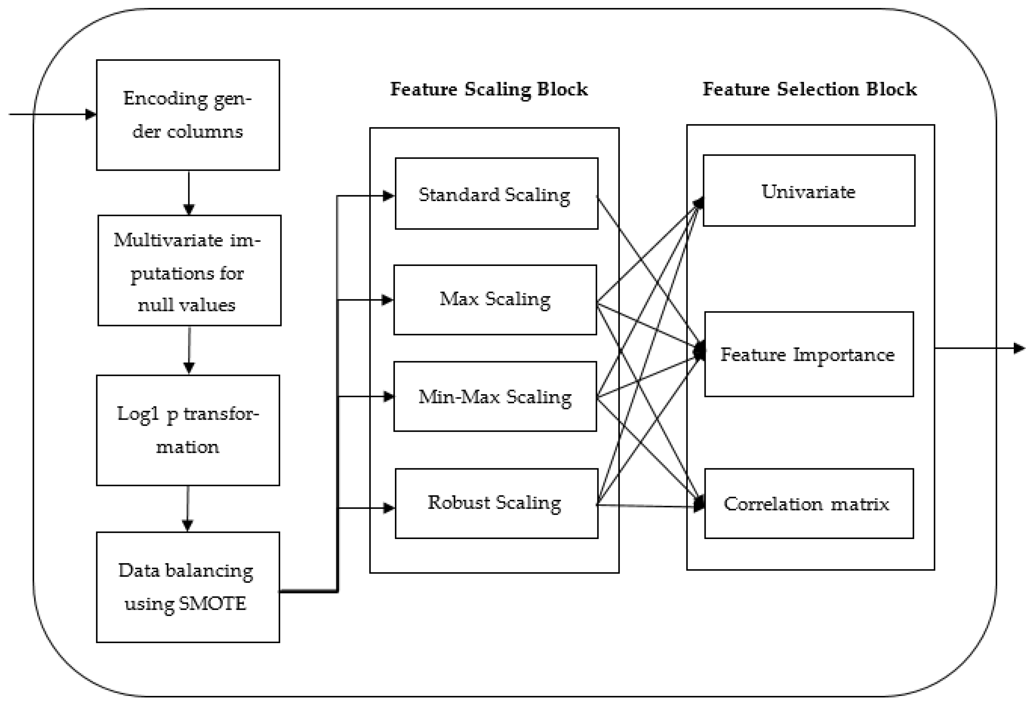
4.2.1. Data Preprocessing
Data Encoding
Data Imputation
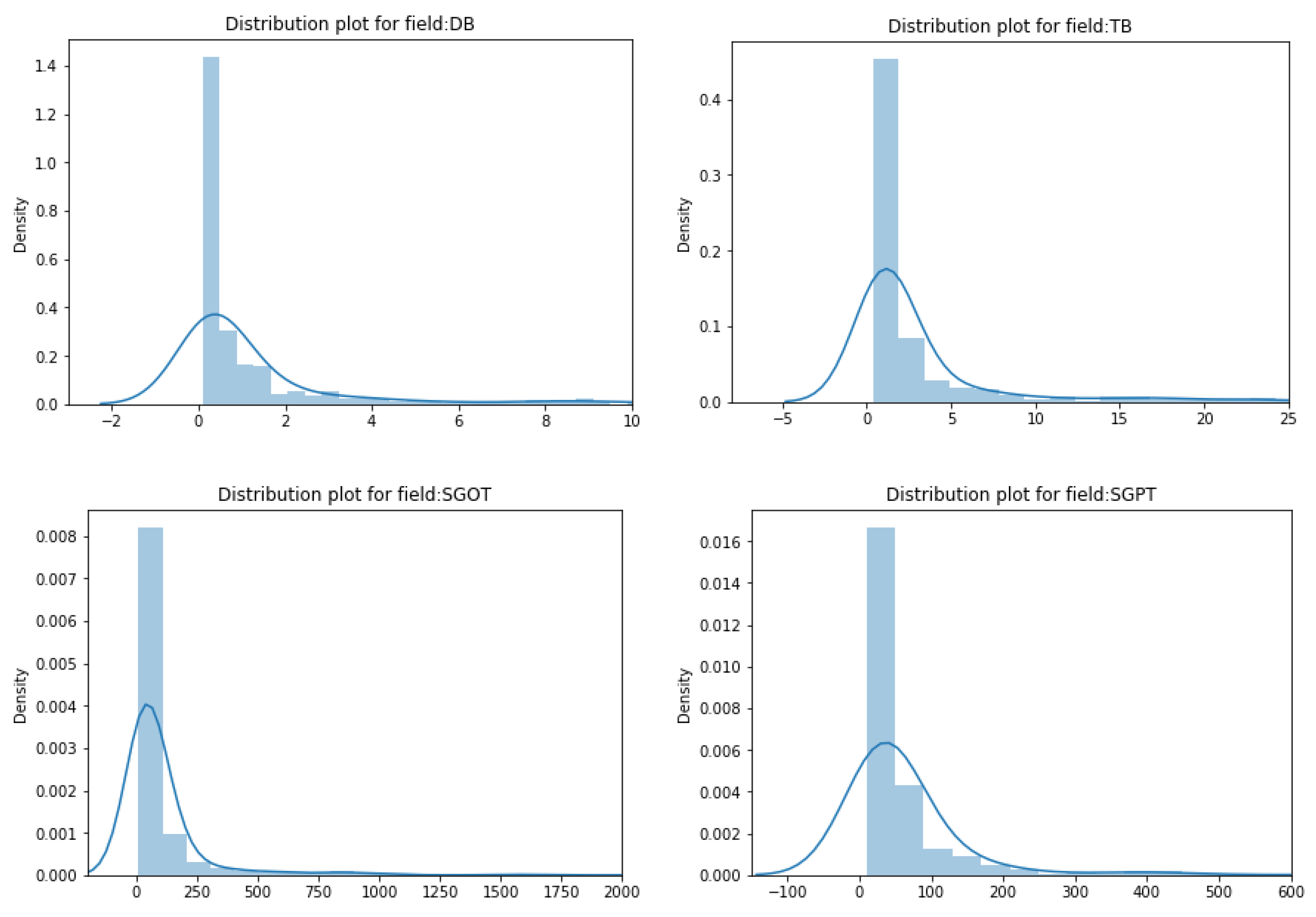
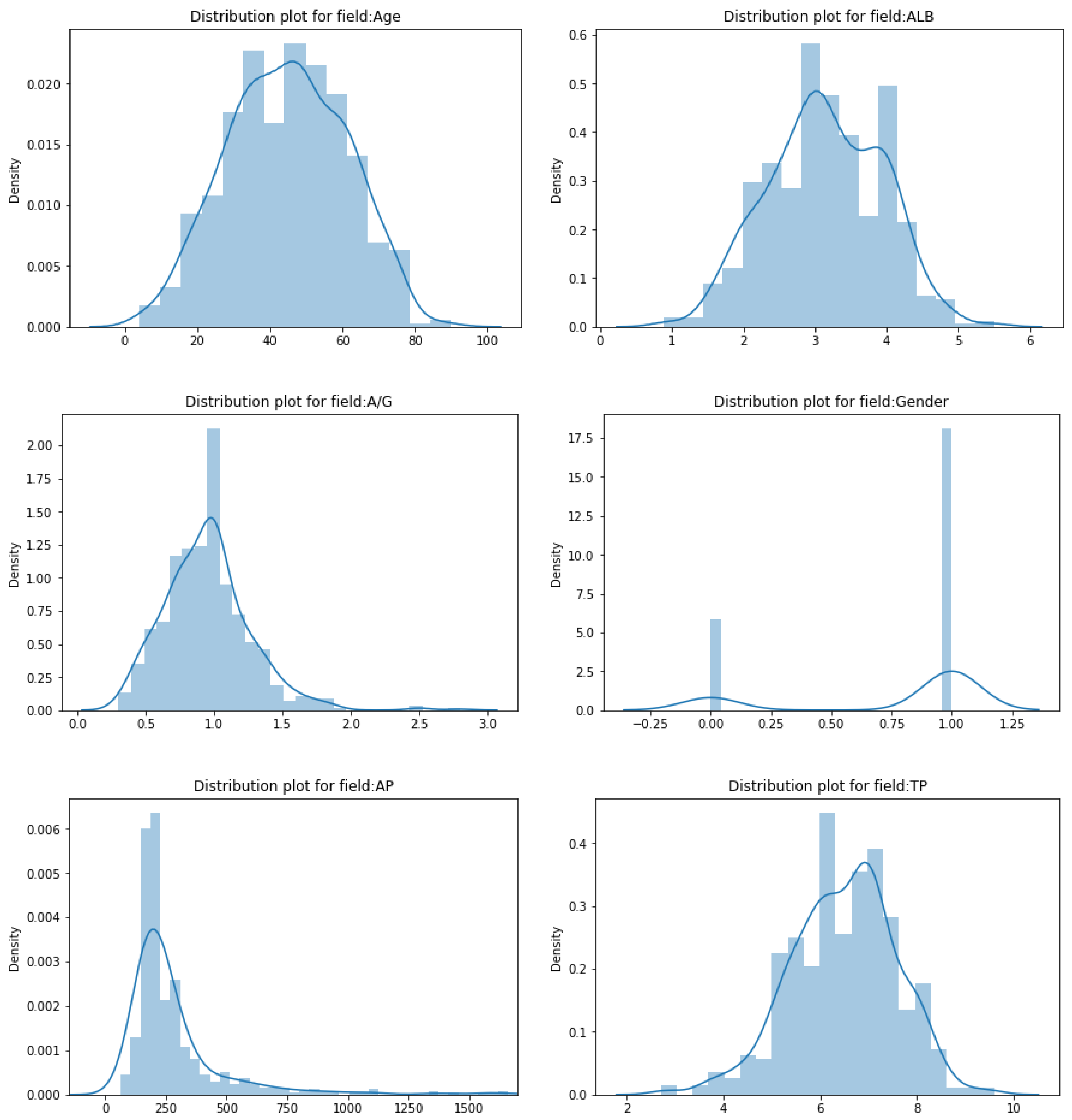
Transforming Skewed Data
Data Balancing
Feature Scaling
- Min–max normalization: This feature scaling method involves shifting and rescaling values to make them fall between 0 and 1. This technique is prone to outliers. The formula used is given in Equation (2).
- Maximum absolute scaling: After applying this technique to features, its value ranges between −1 and +1. In this method, the values in a feature are divided by the absolute max value, as shown in Equation (3).
- Standardization: In standardization, the z value is calculated so the values are rescaled to have a distribution with 0 mean value and variance equal to 1 [26]. The formula used for the standardization is given in Equation (4).
- Robust scaling: It is a feature scaling technique that is robust to outliers. In this method, the feature values are subtracted from their median and divided by the Inter-Quartile Range (IQR) value of that feature. IQR is the difference between Q1 (first quartile) and Q3 (third quartile). The robust scaling formula is given in Equation (5).
Feature Selection
- Univariate feature selection: Univariate statistical tests are used in this strategy to determine the important features. In this, the relationship of a single feature is analyzed with the target variable ignoring other features. Hence, it is called univariate feature selection. From all the scores, features with top scores are selected. There are three tests used for feature selection in this work using the sklearn library. They are the chi-squared test, F-test, and mutual_info_classif test. The chi-squared test is used only for non-negative features and classes. It gauges the interdependence of stochastic variables [28]. The F-test, which is also known as the one-way ANOVA test, is based on the ANOVA F-value. The mutual information is computed for the discrete target variable in the mutual_info_classif test. Mutual information (MI), which evaluates the interdependence between two random variables, is a non-negative value [29].
- Feature importance: The feature importances of each feature of the dataset can be obtained for the target variable using the models. Each data feature is given a score; the higher the score, the more meaningful the feature. To obtain the feature importances of the models, it is trained on the dataset first. Based on the training, the scores are decided. Usually, tree-based classification models are used. In this work, models such as extra tree classifier, random forest, and LGBM classifier were used. All of these models are ensemble models.
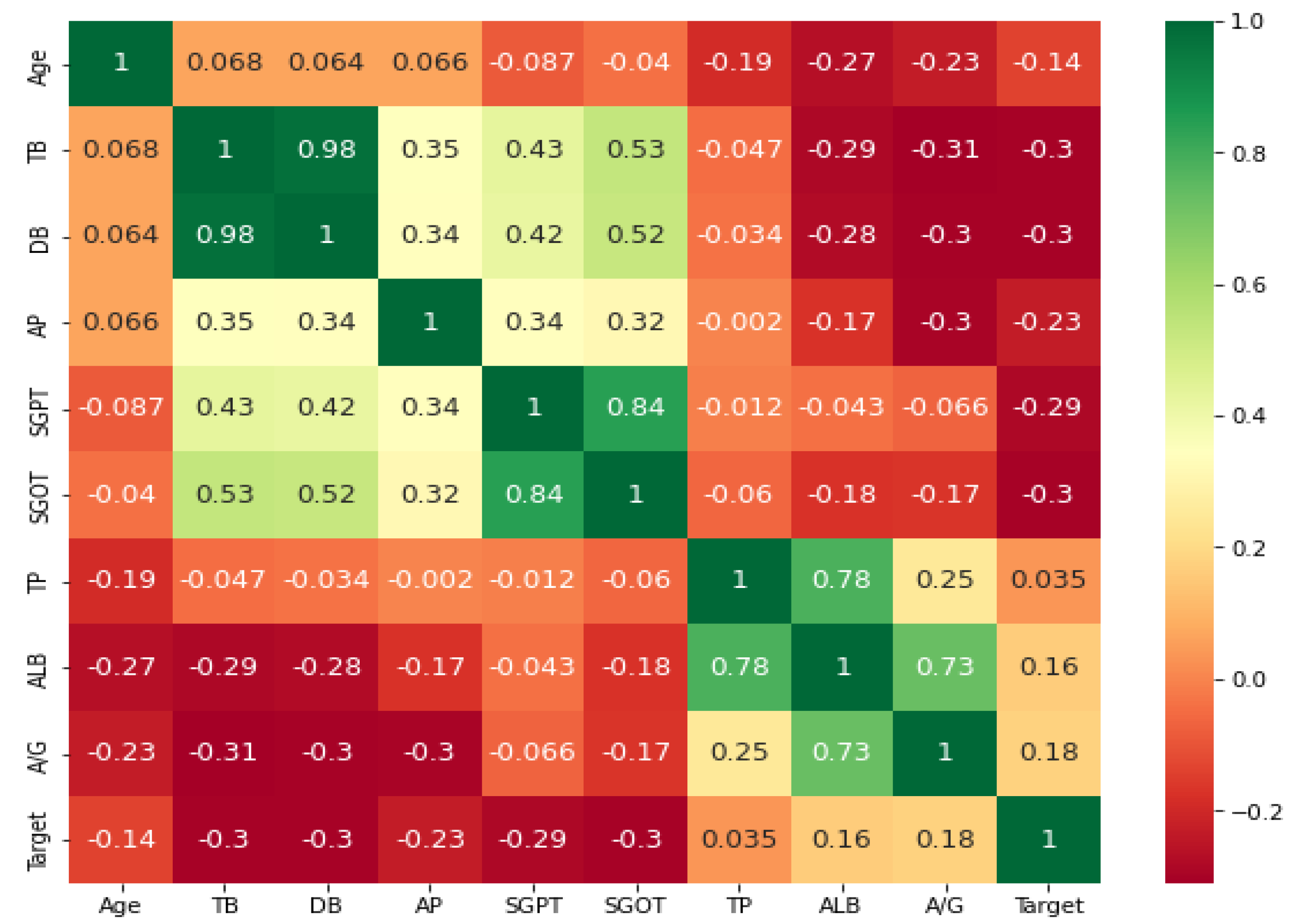
- Correlation coefficient matrix: Correlation is used to determine the relationship between the features or the output variable. It measures the linear relationship between variables. The correlation coefficient can be positive (the output variable value increases as one feature value increases), negative (the output variable value decreases as one feature value increases), or zero (no relation between variables) [30]. The correlation matrix is a matrix containing the correlation value of each feature with every other feature in the dataset including the target. Ideally, features selected should be highly correlated to the target variable and not related to each other, otherwise the feature will not add any additional information. Hence, if two features are correlated, we can remove one of them. Typically, the correlation between characteristics is determined using Pearson’s correlation coefficient.
4.2.2. Machine Learning Algorithms to Predict Liver Disease Using Enhanced Preprocessing
- Performance: A single model may not be able to give reliable results. Combining multiple models helps to increase prediction accuracy [32].
- Robustness: An ensemble helps in reducing the spread in the average performance of the machine learning model [32].
- Low variance: Ensembles help in reducing the variance (error) of the prediction by combining multiple models [32].
Gradient Boosting Classification Algorithm to Predict Liver Disease
- Loss function: It determines how well a model is doing a prediction. More loss means the model could do better and vice versa [34]. Gradient descent is used to minimize this loss function value.
- Weak learner: A weak learner classifies data very poorly and can be comparable to random guessing. It has a high rate of errors. Usually, decision trees are used in this [34].
- Additive model: In this approach, trees are added iteratively and sequentially one at a time. After each iteration, the model is usually closer to the actual target [34].
| Algorithm 1 Gradient Boosting to Predict Liver Disease |
| Input: Training set record Output: Class of record (liver disease or no liver disease) Generating Algorithm Begin Step 1: Calculate the initial log(odds) for the entire dataset Step 2: Calculate the initially predicted probability for each record If the value is greater than 0.5 then positive class else negative class. Step 3: Calculate the Residual for each record Step 4: Build a decision tree with leaves as residuals Step 5: Calculate the output value of the leaf for each record O/P value = Step 6: Calculate the updated log(odds) log(odds) = log(odds) + ( γ X o/p value) Step 7: Calculate the updated predicted probability for each record Repeat steps 3 to 8 till residuals are small or till the number of trees specified Step 8: Calculate the testing probability of each record Step 8.1: Calculate log(odds) log(odds) = log(odds) + ∑ γ × o/p value of leaf Step 8.2: Calculate the predicted probability End |
XGBoosting Classification Algorithm to Predict Liver Disease
Bagging Classification Algorithm to Predict Liver Disease
| Algorithm 2 Bagging to Predict Liver Disease |
| Input: Training set record Output: Class of record (liver disease or no liver disease) Generating Algorithm Begin Step 1: Split data into bootstrap subsets equal to the number of classifiers say n taking all features Step 2: Train n subsets on n base estimators, respectively Step 3: Testing Step 3.1: Calculate the output of the test record on each base learner Step 3.2: Calculate the final predicted value by using the voting method End |
Random Forest Classification Algorithm to Predict Liver Disease
| Algorithm 3 Random Forest Classification to Predict Liver Disease |
| Input: Training set record Output: Class of record (liver disease or no liver disease) Generating Algorithm Begin Step 1: Split data into subsets equal to the number of classifiers say n with random feature selection and best split Step 2: Train n subsets on n decision trees, respectively Step 3: Testing Step 3.1: Calculate the output of the test record on each base learner Step 3.2: Calculate the final predicted value by using the voting method End |
Extra Tree Classification Algorithm to Predict Liver Disease
| Algorithm 4 Extra Tree Classification to Predict Liver Disease |
| Input: Training set record Output: Class of record (liver disease or no liver disease) Generating Algorithm Begin Step 1: Randomly split data into subsets equal to the number of classifiers say n with random feature selection and random-split Step 2: Train n subsets on n decision trees, respectively Step 3: Testing Step 3.1: Calculate the output of the test record on each base learner Step 3.2: Calculate the final predicted value by using the voting method End |
Ensemble Stacking Classification Algorithm to Predict Liver Disease
| Algorithm 5 Ensemble Stacking Classification to Predict Liver Disease |
| Input: Training set record Output: Class of record (liver disease or no liver disease) Generating Algorithm Begin Step 1: Train the entire dataset on n-base learners Step 2: Feed output of base learners to meta learner Base learners used: extra tree classifier, random forest, and xgboost Step 3: Train meta learner on-base learner output Meta learner used: logistic regression Step 4: Testing Step 4.1: Pass each record through base learners Step 4.2: Feed output of base learners to meta learner Step 4.3: Meta-learner output gives final prediction End |
5. Evaluation and Analysis
5.1. Experimental Setup
5.2. Evaluation Metrics
- True Positive (TP)—when positive values are predicted as positive.
- True Negative (TN)—when negative values are predicted as negative.
- False Positive (FP)—when negative values are predicted as positive.
- False Negative (FN)—when positive values are predicted as negative.
5.3. Experimental Results
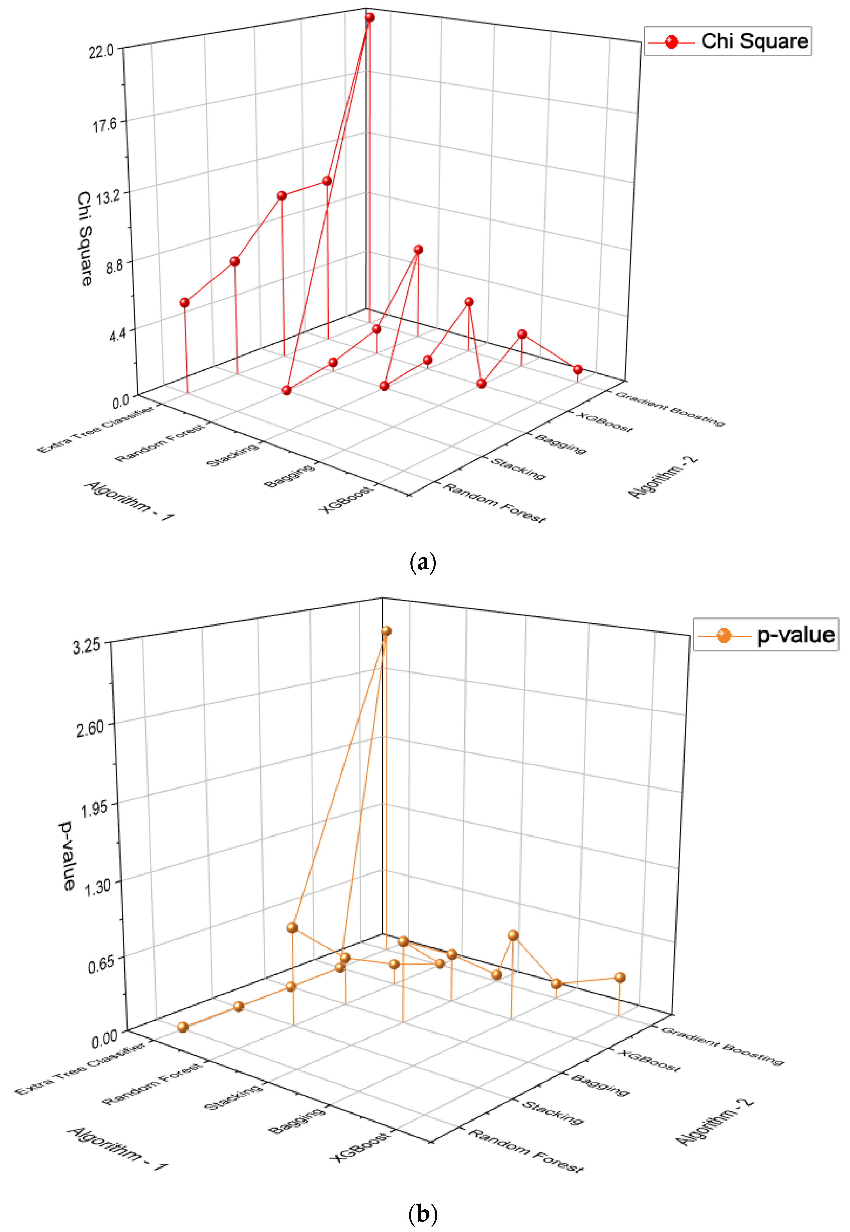
5.3.1. Statistical Test Results
5.3.2. Visualization of Features
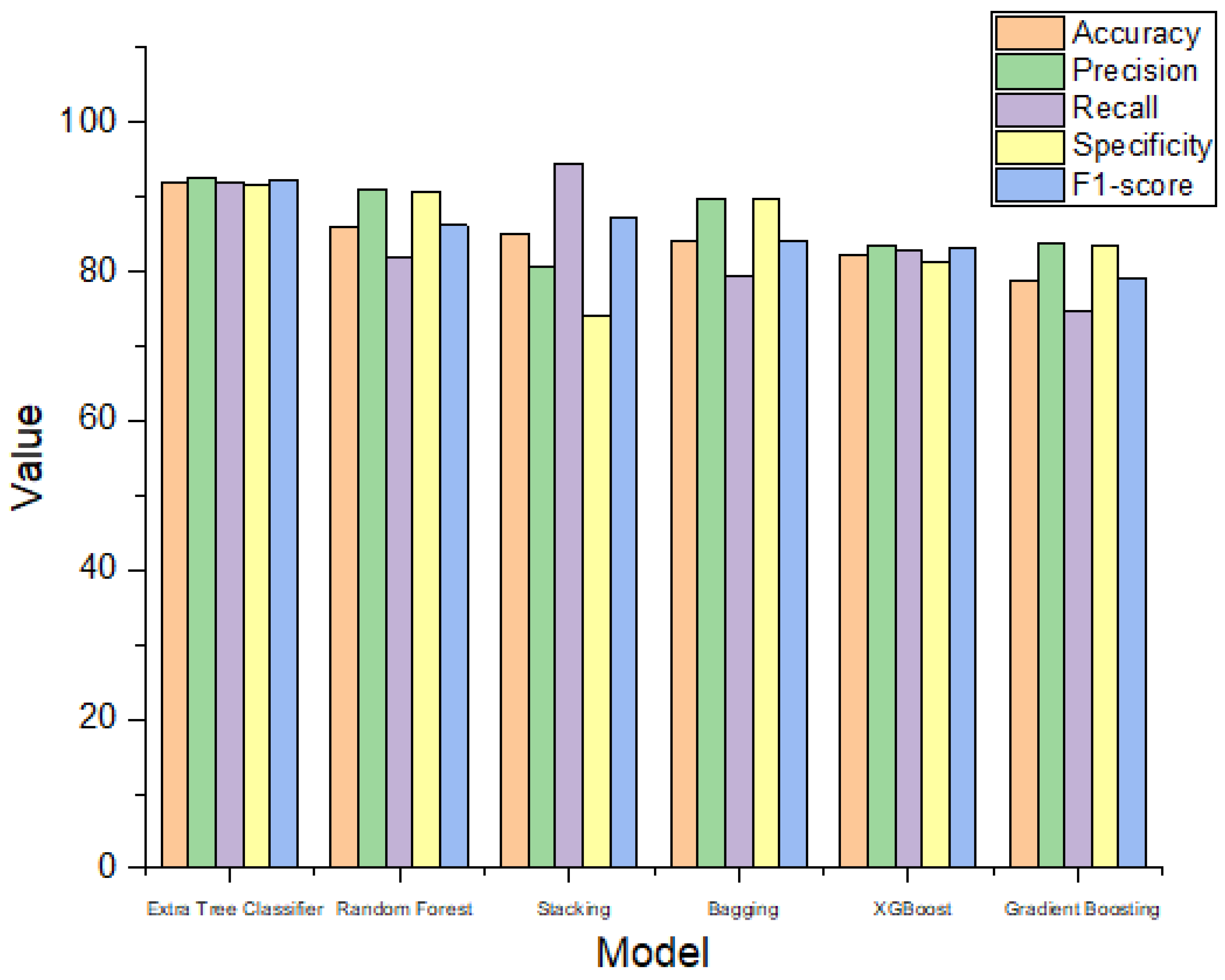
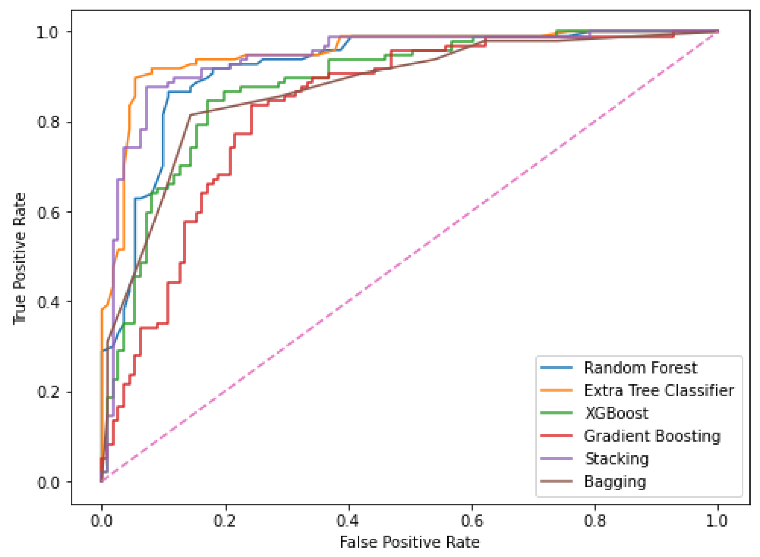
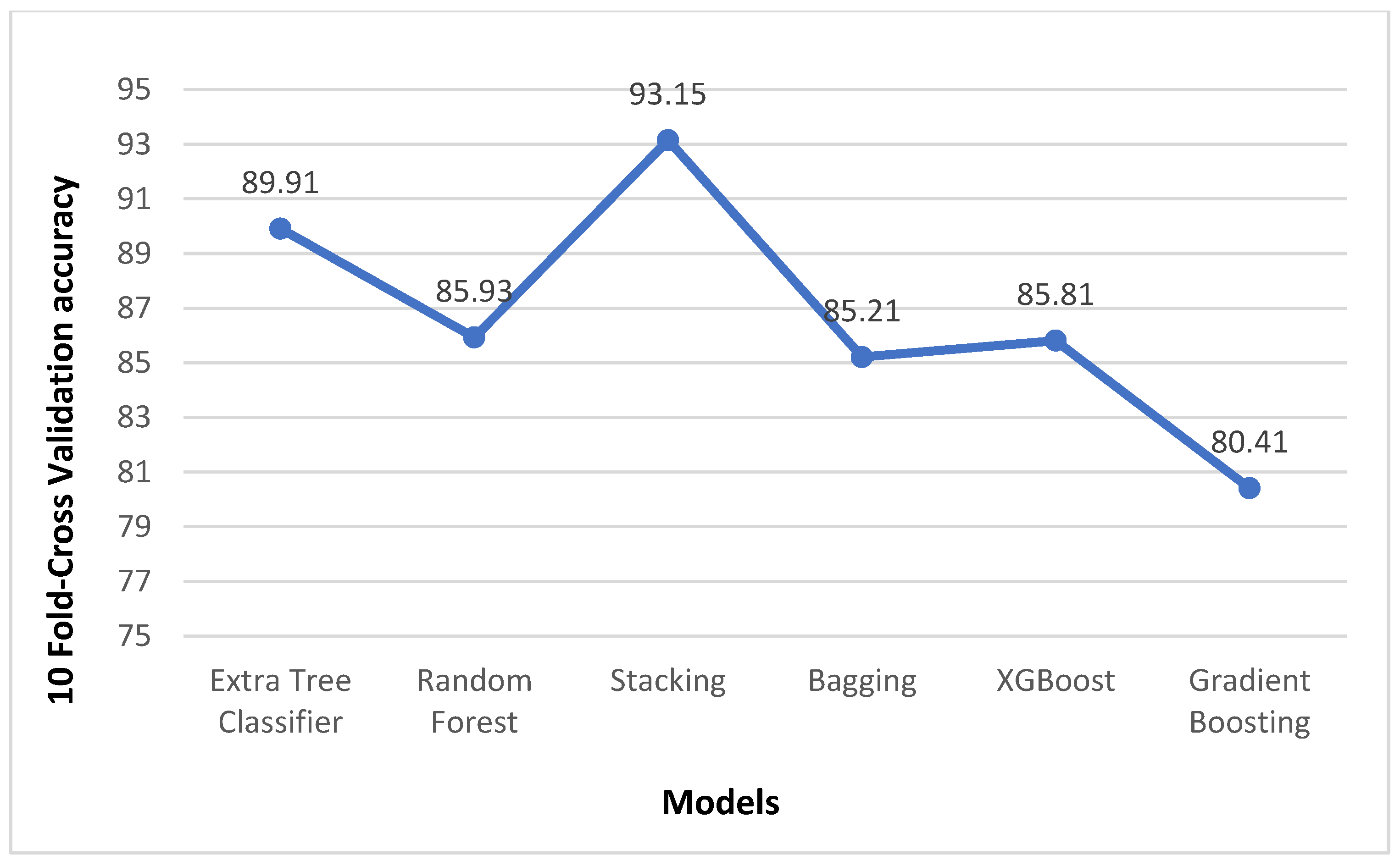
5.4. Performance Comparison
6. Conclusions
Author Contributions
Funding
Institutional Review Board Statement
Informed Consent Statement
Data Availability Statement
Acknowledgments
Conflicts of Interest
References
- “Liver Disease in India,” World Life Expectancy. Available online: https://www.worldlifeexpectancy.com/india-liver-disease (accessed on 14 April 2022).
- Sindhuja, D.R.J.P.; Priyadarsini, R.J. A survey on classification techniques in data mining for analyzing liver disease disorder. Int. J. Comput. Sci. Mob. Comput. 2016, 5, 483–488. [Google Scholar]
- Shaheamlung, G.; Kaur, H.; Kaur, M. A Survey on machine learning techniques for the diagnosis of liver disease. In Proceedings of the 2020 International Conference on Intelligent Engineering and Management (ICIEM), London, UK, 17–19 June 2020. [Google Scholar]
- Sun, Q.-F.; Ding, J.-G.; Xu, D.-Z.; Chen, Y.-P.; Hong, L.; Ye, Z.-Y.; Zheng, M.-H.; Fu, R.-Q.; Wu, J.-G.; Du, Q.-W.; et al. Prediction of the prognosis of patients with acute-on-chronic hepatitis B liver failure using the model for end-stage liver disease scoring system and a novel logistic regression model. J. Viral Hepat. 2009, 16, 464–470. [Google Scholar] [CrossRef] [PubMed]
- Liu, K.-H.; Huang, D.-S. Cancer classification using Rotation Forest. Comput. Biol. Med. 2008, 38, 601–610. [Google Scholar] [CrossRef]
- Ramana, B.V.; Babu, M.S.P.; Venkateswarlu, N.B. A critical study of selected classification algorithms for liver disease diagnosis. Int. J. Database Manag. Syst. 2011, 3, 101–114. [Google Scholar] [CrossRef]
- Ramana, B.V.; Babu, M.P.; Venkateswarlu, N.B. Liver classification using modified rotation forest. Int. J. Eng. Res. Dev. 2012, 6, 17–24. [Google Scholar]
- Kumar, Y.; Sahoo, G. Prediction of different types of liver diseases using rule based classification model. Technol. Health Care 2013, 21, 417–432. [Google Scholar] [CrossRef] [PubMed]
- Ayeldeen, H.; Shaker, O.; Ayeldeen, G.; Anwar, K.M. Prediction of liver fibrosis stages by machine learning model: A decision tree approach. In Proceedings of the 2015 Third World Conference on Complex Systems (WCCS), Marrakech, Morocco, 23–25 November 2015. [Google Scholar]
- Hashem, S.; Esmat, G.; Elakel, W.; Habashy, S.; Raouf, S.A.; Elhefnawi, M.; Eladawy, M.; ElHefnawi, M. Comparison of machine learning approaches for prediction of advanced liver fibrosis in chronic hepatitis C patients. IEEE/ACM Trans. Comput. Biol. Bioinform. 2018, 15, 861–868. [Google Scholar]
- Sontakke, S.; Lohokare, J.; Dani, R. Diagnosis of liver diseases using machine learning. In Proceedings of the 2017 International Conference on Emerging Trends & Innovation in ICT (ICEI), Pune, India, 3–5 February 2017. [Google Scholar]
- Ma, H.; Xu, C.-F.; Shen, Z.; Yu, C.-H.; Li, Y.-M. Application of machine learning techniques for clinical predictive modeling: A cross-sectional study on nonalcoholic fatty liver disease in China. Biomed. Res. Int. 2018, 2018, 4304376. [Google Scholar] [CrossRef] [PubMed] [Green Version]
- Jacob, J.; Mathew, J.C.; Mathew, J.; Issac, E. Diagnosis of liver disease using machine learning techniques. Int. Res. J. Eng. Technol. 2018, 5, 412–423. [Google Scholar]
- Sivakumar, D.; Varchagall, M.; Gusha, S.A. Chronic Liver Disease Prediction Analysis Based on the Impact of Life Quality Attributes. Int. J. Recent Technol. Eng. (IJRTE) 2019, 7, 2111–2117. [Google Scholar]
- Durai, V.; Ramesh, S.; Kalthireddy, D. Liver disease prediction using machine learning. Int. J. Adv. Res. Ideas Innov. Technol. 2019, 5, 1584–1588. [Google Scholar]
- Gogi, V.J. Prognosis of Liver Disease: Using Machine Learning Algorithms. In Proceedings of the Conference on Recent Innovations in Electrical, Electronics & Communication Engineering (ICRIEECE), Bhubaneswar, India, 27–28 July 2018. [Google Scholar]
- Ambesange, S.; Vijayalaxmi; Uppin, R.; Patil, S.; Patil, V. Optimizing Liver disease prediction with Random Forest by various Data balancing Techniques. In Proceedings of the 2020 IEEE International Conference on Cloud Computing in Emerging Markets (CCEM), Bengaluru, India, 6–7 November 2020. [Google Scholar]
- Geetha, C.; Arunachalam, A.R. Evaluation based Approaches for Liver Disease Prediction using Machine Learning Algorithms. In Proceedings of the 2021 International Conference on Computer Communication and Informatics (ICCCI), Coimbatore, India, 27–29 January 2021. [Google Scholar]
- Lin, R.-H. An intelligent model for liver disease diagnosis. Artif. Intell. Med. 2009, 47, 53–62. [Google Scholar] [CrossRef] [PubMed]
- Kim, Y.S.; Sohn, S.Y.; Kim, D.K.; Kim, D.; Paik, Y.H.; Shim, H.S. Screening test data analysis for liver disease prediction model using growth curve. Biomed. Pharmacother. 2003, 57, 482–488. [Google Scholar] [CrossRef] [PubMed]
- Wu, C.-C.; Yeh, W.-C.; Hsu, W.-D.; Islam, M.; Nguyen, P.A.; Poly, T.N.; Wang, Y.-C.; Yang, H.-C.; Li, Y.-C. Prediction of fatty liver disease using machine learning algorithms. Comput. Methods Programs Biomed. 2019, 170, 23–29. [Google Scholar] [CrossRef] [PubMed]
- “UCI Machine Learning Repository: ILPD (Indian Liver Patient Dataset) Data Set,” Uci.edu. Available online: https://archive.ics.uci.edu/ml/datasets/ILPD+(Indian+Liver+Patient+Dataset) (accessed on 14 April 2022).
- “6.4. Imputation of Missing Values,” Scikit-Learn. Available online: https://scikit-learn.org/stable/modules/impute.html (accessed on 14 April 2022).
- “Transforming Skewed Data for machine Learning,” Open Data Science—Your News Source for AI, Machine Learning & More. 24 June 2019. Available online: https://opendatascience.com/transforming-skewed-data-for-machine-learning/ (accessed on 14 April 2022).
- “ML,” GeeksforGeeks. 2 July 2018. Available online: https://www.geeksforgeeks.org/ml-feature-scaling-part-2 (accessed on 14 April 2022).
- Eddie_, “Feature Scaling Techniques,” Analytics Vidhya. 18 May 2021. Available online: https://www.analyticsvidhya.com/blog/2021/05/feature-scaling-techniques-in-python-a-complete-guide/ (accessed on 14 April 2022).
- “Sklearn.Feature_Selection.Chi2,” Scikit-Learn. Available online: https://scikit-learn.org/stable/modules/generated/sklearn.feature_selection.chi2.html (accessed on 14 April 2022).
- “Sklearn.Feature_Selection.Mutual_info_Classif,” Scikit-Learn. Available online: https://scikit-learn.org/stable/modules/generated/sklearn.feature_selection.mutual_info_classif.html (accessed on 14 April 2022).
- Shaikh, R. Feature Selection Techniques in Machine Learning with Python. Towards Data Science. 28 October 2018. Available online: https://towardsdatascience.com/feature-selection-techniques-in-machine-learning-with-python-f24e7da3f36e (accessed on 14 April 2022).
- Alhamid, M. Ensemble Models. Towards Data Science. 15 March 2021. Available online: https://towardsdatascience.com/ensemble-models-5a62d4f4cb0c (accessed on 14 April 2022).
- Brownlee, J. Why Use Ensemble Learning? Machine Learning Mastery. 25 October 2020. Available online: https://machinelearningmastery.com/why-use-ensemble-learning/ (accessed on 14 April 2022).
- Nelson, D. Gradient Boosting Classifiers in Python with Scikit-Learn. Stack Abuse. 17 July 2019. Available online: https://stackabuse.com/gradient-boosting-classifiers-in-python-with-scikit-learn/ (accessed on 14 April 2022).
- Kurama, V. Gradient Boosting for Classification. Paperspace Blog. 29 March 2020. Available online: https://blog.paperspace.com/gradient-boosting-for-classification/ (accessed on 14 April 2022).
- Morde, V. XGBoost Algorithm: Long May She Reign! Towards Data Science. 8 April 2019. Available online: https://towardsdatascience.com/https-medium-com-vishalmorde-xgboost-algorithm-long-she-may-rein-edd9f99be63d (accessed on 14 April 2022).
- Nelson, D. Ensemble/Voting Classification in Python with Scikit-Learn. Stack Abuse. 22 January 2020. Available online: https://stackabuse.com/ensemble-voting-classification-in-python-with-scikit-learn/ (accessed on 14 April 2022).
- Le, N.Q.K.; Ho, Q.-T.; Nguyen, V.-N.; Chang, J.-S. BERT-Promoter: An improved sequence-based predictor of DNA promoter using BERT pre-trained model and SHAP feature selection. Comput. Biol. Chem. 2022, 99, 107732. [Google Scholar] [CrossRef] [PubMed]
- Kha, Q.-H.; Ho, Q.-T.; Le, N.Q.K. Identifying SNARE proteins using an alignment-free method based on multiscan convolutional neural network and PSSM profiles. J. Chem. Inf. Model. 2022, 62, 4820–4826. [Google Scholar] [CrossRef] [PubMed]
- Raschka, S. Model evaluation, model selection, and algorithm selection in machine learning. arXiv 2018. [Google Scholar] [CrossRef]
- Raschka, S. Ftest: F-Test for Classifier Comparisons. Github.io. Available online: http://rasbt.github.io/mlxtend/user_guide/evaluate/ftest/ (accessed on 29 January 2023).
- Srivenkatesh, D.M. Performance evolution of different machine learning algorithms for prediction of liver disease. Int. J. Innov. Technol. Explor. Eng. 2019, 9, 1115–1122. [Google Scholar] [CrossRef]


| Characteristics | Patients | ||||||
|---|---|---|---|---|---|---|---|
| All | With Liver Disease | Without Liver Disease | |||||
| Number | % | Number | % | Number | % | ||
| Patients Enrolled | 583 | 100 | 416 | 71.36 | 167 | 28.65 | |
| Age (in years) | Median | 45 | 46 | 40 | |||
| Range | 4 to 90 | 7 to 90 | 4 to 85 | ||||
| Gender | Male | 441 | 75.64 | 324 | 77.88 | 117 | 70.06 |
| Female | 142 | 24.36 | 92 | 22.12 | 50 | 29.94 | |
| Total Bilirubin (TB) | Median | 1 | 1.4 | 0.8 | |||
| Range | 0.4 to 75 | 0.4 to 75 | 0.5 to 7.3 | ||||
| Direct Bilirubin(DB) | Median | 0.3 | 0.5 | 0.2 | |||
| Range | 0.1 to 19.7 | 0.1 to 19.7 | 0.1 to 3.6 | ||||
| Alkaline Phosphotase(AP) | Median | 208 | 229 | 186 | |||
| Range | 63 to 2110 | 63 to 2110 | 90 to 1590 | ||||
| Alamine Aminotransferase (SGPT) | Median | 35 | 41 | 27 | |||
| Range | 10 to 2000 | 12 to 2000 | 10 to 181 | ||||
| Aspartate Aminotransferase (SGOT) | Median | 42 | 52.5 | 29 | |||
| Range | 4 to 4929 | 11 to 4929 | 10 to 285 | ||||
| Total Proteins (TP) | Median | 6.6 | 6.55 | 6.6 | |||
| Range | 2.7 to 9.6 | 2.7 to 9.6 | 3.7 to 9.2 | ||||
| Albumin | Median | 3.10 | 3.00 | 3.4 | |||
| Range | 0.9 to 5.5 | 0.9 to 5.5 | 1.4 to 5.0 | ||||
| Albumin and Globulin Ratio | Median | 0.93 | 0.90 | 1 | |||
| Range | 0.3 to 2.8 | 0.3 to 2.8 | 0.37 to 1.9 | ||||
| Ensemble Models | Ranges of Hyperparameters | Optimal Value |
|---|---|---|
| Random Forest | n_estimators: [100, 150, 200, 500] | 100 |
| criterion: [gini, entropy] | gini | |
| min_samples_split: [1.0, 2, 4, 5] | 2 | |
| min_samples_leaf: [1, 2, 4, 5] | 1 | |
| max_leaf_nodes: [4, 10, 20, 50, None] | None | |
| Extra Tree Classifier | n_estimators: [100, 150, 200, 500] | 100 |
| criterion: [gini, entropy] | entropy | |
| min_samples_split: [1.0, 2, 4,5] | 2 | |
| min_samples_leaf: [1, 2, 4, 5] | 1 | |
| max_leaf_nodes: [4, 10, 20, 50, None] | None | |
| XGBoost | n_estimators: [100, 200, 500] | 500 |
| learning_rate: [0.01, 0.05, 0.1] | 0.05 | |
| booster: [gbtree, gblinear] | gbtree | |
| gamma: [0, 0.5, 1] | 0 | |
| reg_alpha: [0, 0.5, 1] | 0 | |
| ‘reg_lambda’: [0.5, 1, 5] | 0.5 | |
| ‘base_score’: [0.2, 0.5, 1] | 0.2 | |
| Gradient Boosting | ‘n_estimators’: [100, 200, 500], | 200 |
| ‘learning_rate’: [0.1, 0.2, 0.5], | 0.5 | |
| ‘criterion’: [‘friedman_mse’, ’mse’, ‘mae’], | friedman_mse | |
| ‘min_samples_split’: [2, 4, 5], | 2 | |
| ‘min_samples_leaf’: [1, 2, 4, 5] | 1 | |
| Bagging | ‘n_estimators’: [100, 200, 300] | 200 |
| Algorithm | Accuracy (95% CI) | Precision (95% CI) | Recall (95% CI) | Specificity (95% CI) |
|---|---|---|---|---|
| Extra Tree Classifier | 91.82 (87.88–95.19) | 92.72 (87.50–97.17) | 91.89 (86.54–96.43) | 91.75 (85.44–95.48) |
| Random Forest | 86.06 (81.25–90.38) | 91.00 (85.00–96.04) | 81.98 (74.54–88.50) | 90.72 (84.27–95.79) |
| Stacking | 85.10 (80.29–89.44) | 80.76 (73.55–87.50) | 94.59 (90.10–98.15) | 74.22 (64.83–82.05) |
| Bagging | 84.13 (78.85–88.47) | 89.79 (83.33–95.56) | 79.27 (71.31–86.33) | 89.69 (82.95–95.40) |
| XGBoost | 82.21 (76.92–87.50) | 83.63 (76.72–90.27) | 82.88 (75.73–90.09) | 81.44 (73.33–88.79) |
| Gradient Boosting | 78.85 (73.08–84.13) | 83.83 (76.29–90.91) | 74.77 (66.09–82.24) | 83.50 (76.19–90.39) |
| Algorithm | F1-Score | ROC_AUC | 10-Fold Cross Validation Accuracy |
|---|---|---|---|
| Extra Tree Classifier | 92.30 | 91.82 | 89.91 |
| Random Forest | 86.25 | 86.35 | 85.93 |
| Stacking | 87.13 | 84.41 | 93.15 |
| Bagging | 84.21 | 84.48 | 85.21 |
| XGBoost | 83.25 | 82.16 | 85.81 |
| Gradient Boosting | 79.04 | 79.13 | 80.41 |
| S. No. | Features | Scores |
|---|---|---|
| 1 | DB | 129.48 |
| 2 | TB | 121.47 |
| 3 | SGOT | 98.36 |
| 4 | SGPT | 92.54 |
| 5 | AP | 83.92 |
| 6 | A/G | 54.79 |
| 7 | ALB | 31.55 |
| 8 | Age | 13.34 |
| 9 | Gender | 03.69 |
| 10 | TP | 00.29 |
| Algorithm 1 | Algorithm 2 | Chi-Square | p-Value |
|---|---|---|---|
| Extra Tree Classifier | Random Forest | 6.05 | 0.0139 |
| Extra Tree Classifier | Stacking | 7.6818 | 0.0055 |
| Extra Tree Classifier | Bagging | 11.1304 | 0.0008 |
| Extra Tree Classifier | XGBoost | 11.2813 | 0.0008 |
| Extra Tree Classifier | Gradient Boosting | 21.8064 | 3.0158 |
| Random Forest | Stacking | 0.0294 | 0.8638 |
| Random Forest | Bagging | 0.64 | 0.4237 |
| Random Forest | XGBoost | 1.75 | 0.1859 |
| Random Forest | Gradient Boosting | 6.3226 | 0.0119 |
| Stacking | Bagging | 0.1290 | 0.7194 |
| Stacking | XGBoost | 0.625 | 0.4292 |
| Stacking | Gradient Boosting | 3.5122 | 0.0609 |
| Bagging | XGBoost | 0.1026 | 0.7488 |
| Bagging | Gradient Boosting | 2.25 | 0.1336 |
| XGBoost | Gradient Boosting | 0.8780 | 0.3487 |
| S. No. | Source | Algorithm | Accuracy (in %) |
|---|---|---|---|
| 1 | Bendi et al. [7] | Bayesian Network | 71.30 |
| 2 | Bendi et al. [7] | MLP | 71.53 |
| 3 | Bendi et al. [7] | KStar | 73.07 |
| 4 | Sumedh et al. [12] | Back Propagation | 73.2 |
| 5 | Srivenkatesh et al. [40] | Random Forest | 74.57 |
| 6 | Geetha et al. [19] | SVM | 75.04 |
| 7 | Srivenkatesh et al. [40] | Logistic Regression | 76.27 |
| 8 | Ensemble Learning (EL) With Enhanced Preprocessing (EP) | Random Forest | 86.06 |
| 9 | Ensemble Learning (EL) With Enhanced Preprocessing (EP) | Extra Tree Classifier | 91.82 |
Disclaimer/Publisher’s Note: The statements, opinions and data contained in all publications are solely those of the individual author(s) and contributor(s) and not of MDPI and/or the editor(s). MDPI and/or the editor(s) disclaim responsibility for any injury to people or property resulting from any ideas, methods, instructions or products referred to in the content. |
© 2023 by the authors. Licensee MDPI, Basel, Switzerland. This article is an open access article distributed under the terms and conditions of the Creative Commons Attribution (CC BY) license (https://creativecommons.org/licenses/by/4.0/).
Share and Cite
Md, A.Q.; Kulkarni, S.; Joshua, C.J.; Vaichole, T.; Mohan, S.; Iwendi, C. Enhanced Preprocessing Approach Using Ensemble Machine Learning Algorithms for Detecting Liver Disease. Biomedicines 2023, 11, 581. https://doi.org/10.3390/biomedicines11020581
Md AQ, Kulkarni S, Joshua CJ, Vaichole T, Mohan S, Iwendi C. Enhanced Preprocessing Approach Using Ensemble Machine Learning Algorithms for Detecting Liver Disease. Biomedicines. 2023; 11(2):581. https://doi.org/10.3390/biomedicines11020581
Chicago/Turabian StyleMd, Abdul Quadir, Sanika Kulkarni, Christy Jackson Joshua, Tejas Vaichole, Senthilkumar Mohan, and Celestine Iwendi. 2023. "Enhanced Preprocessing Approach Using Ensemble Machine Learning Algorithms for Detecting Liver Disease" Biomedicines 11, no. 2: 581. https://doi.org/10.3390/biomedicines11020581