
“Realistic Choice of Annual Matrices Contracts the Range of λS Estimates” under Reproductive Uncertainty Too


Abstract
:1. Introduction
2. Materials and Methods
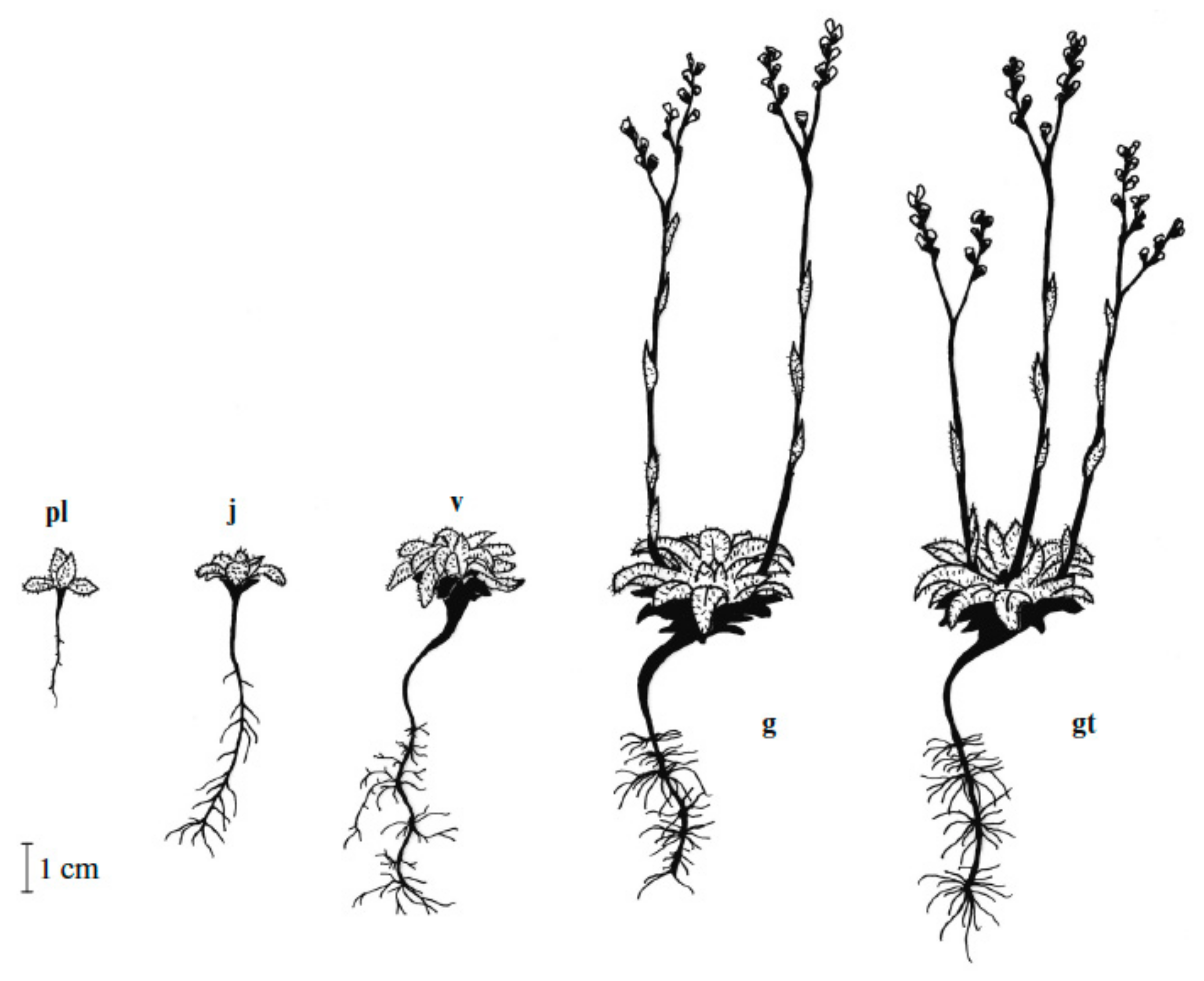
2.1. Case Study of Eritrichium Caucasicum
- –
- –
- –
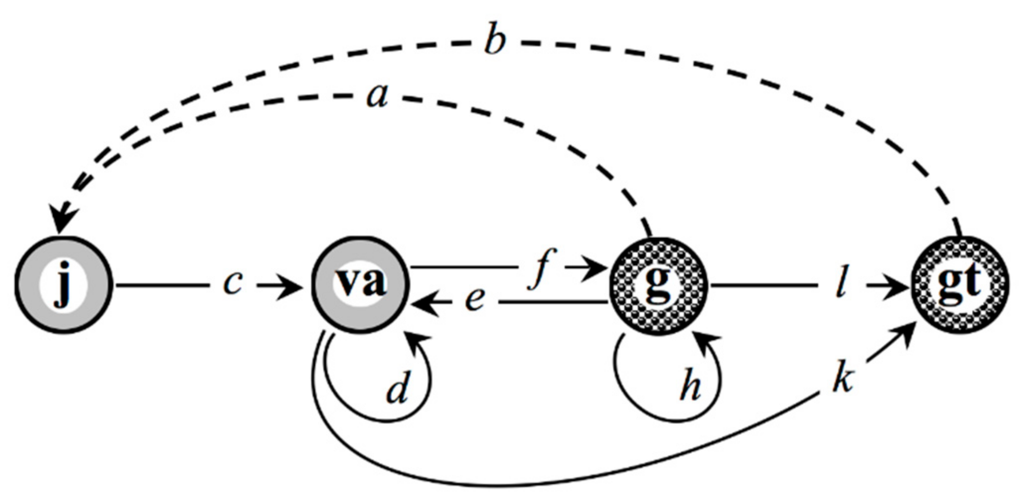
- accelerated transitions va ⤻ gt as a manifestation of polyvariant ontogeny in E. caucasicum under the conditions of the alpine belt in north-western Caucasus.
2.2. Stochastic Growth Rate, λS
2.3. Local Meteodata, Statistical Treatment
2.4. Revealing the Pattern of Transition Matrix and Estimating Its Elements
2.5. Estimating λS by the Direct MC Method with a Markov Chain
3. Results
3.1. Transition Matrix of the Governing Markov Chain
3.2. Estimates of λS
4. Discussion
5. Conclusions
Supplementary Materials
Author Contributions
Funding
Acknowledgments
Conflicts of Interest
Appendix A. Diverging/Vanishing Sequences and a Remedy to Cope with
References
- Logofet, D.O.; Golubyatnikov, L.L.; Ulanova, N.G. Realistic choice of annual matrices contracts the range of λS estimates. Mathematics 2020, 8, 2252. [Google Scholar] [CrossRef]
- Caswell, H. Matrix Population Models: Construction, Analysis and Interpretation, 2nd ed.; Sinauer Associates: Sunderland, MA, USA, 2001. [Google Scholar]
- Logofet, D.O. Projection matrices revisited: A potential-growth indicator and the merit of indication. J. Math. Sci. 2013, 193, 671–686. [Google Scholar] [CrossRef]
- Horn, R.A.; Johnson, C.R. Matrix Analysis; Cambridge University Press: Cambridge, UK, 1990. [Google Scholar]
- Logofet, D.O. Matrices and Graphs: Stability Problems in Mathematical Ecology; CRC Press: Boca Raton, FL, USA, 1993. [Google Scholar]
- Logofet, D.O.; Ulanova, N.G.; Belova, I.N. Adaptation on the ground and beneath: Does the local population maximize its λ1? Ecol. Complex. 2014, 20, 176–184. [Google Scholar] [CrossRef]
- Logofet, D.O. Projection matrices in variable environments: λ1 in theory and practice. Ecol. Model. 2013, 251, 307–311. [Google Scholar] [CrossRef]
- Logofet, D.O.; Kazantseva, E.S.; Belova, I.N.; Onipchenko, V.G. Local population of Eritrichium caucasicum as an object of mathematical modelling. I. Life cycle graph and a nonautonomous matrix model. Biol. Bull. Rev. 2017, 7, 415–427. [Google Scholar] [CrossRef]
- Logofet, D.O.; Kazantseva, E.S.; Belova, I.N.; Onipchenko, V.G. Local population of Eritrichium caucasicum as an object of mathematical modelling. II. How short does the short-lived perennial live? Biol. Bull. Rev. 2018, 8, 415–427. [Google Scholar] [CrossRef]
- Logofet, D.O. Convexity in projection matrices: Projection to a calibration problem. Ecol. Model. 2008, 216, 217–228. [Google Scholar] [CrossRef]
- Logofet, D.O.; Kazantseva, E.S.; Belova, I.N.; Onipchenko, V.G. How long does a short-lived perennial live? A modelling approach. Biol. Bull. Rev. 2018, 8, 406–420. [Google Scholar] [CrossRef]
- Logofet, D.O.; Kazantseva, E.S.; Belova, I.N.; Onipchenko, V.G. Local population of Eritrichium caucasicum as an object of mathematical modelling. III. Population growth in the random environment. Biol. Bull. Rev. 2019, 9, 453–464. [Google Scholar] [CrossRef]
- Tuljapurkar, S.D. Population Dynamics in Variable Environments; Springer: New York, NY, USA, 1990. [Google Scholar]
- Kazantseva, E.S. Population Dynamics and Seed Productivity of Short-Lived Alpine Plants in the North-West Caucasus. Candidate of Science (Biology) Dissertation, Moscow State University, Moscow, Russia, 2016. (In Russian). [Google Scholar]
- Körner, C. Alpine Plant Life: Functional Plant Ecology of High Mountain Ecosystems, 2nd ed.; Springer: Berlin/Heidelberg, Germany, 2003. [Google Scholar]
- Rabonov, T.A. Life Cycle of Perennial Herbaceous Plants in Meadow Phytocoenoses; Tr. BIN Academy of Sciences of the USSR. Geobotany. USSR Academy of Sciences: Moscow, Russia, 1950; Volume 6, pp. 7–204. (In Russian) [Google Scholar]
- Rabotnov, T.A. Fitotsenologiya (Phytocenology); Moscow State University Publisher: Moscow, Russia, 1978. (In Russian) [Google Scholar]
- Bender, M.H.; Baskin, J.M.; Baskin, C.C. Age of maturity and life span in herbaceous, polycarpic perennials. Bot. Rev. 2000, 66, 311–349. [Google Scholar] [CrossRef]
- Keller, R.; Vittoz, P. Clonal growth and demography of a hemicryptophyte alpine plant: Leontopodium alpinum Cassini. Alp. Bot. 2015, 125, 31–40. [Google Scholar] [CrossRef]
- Nakhutsrishvili, G.S.; Gamtsemlidze, Z.G. Zhizn’ Rastenii v Extremal’nykh Usloviyakh Vysokogorii: Na Primere Tsentralnogo Kavkasa (Plant Life in Extreme High Altitude Conditions by Example of the Central Caucasus); Nauka: Leningrad, Russia, 1984. [Google Scholar]
- Onipchenko, V.G. (Ed.) Alpine Ecosystems in the Northwest Caucasus; Kluwer: Dordrecht, The Netherlands, 2004. [Google Scholar]
- Furstenberg, H.; Kesten, H. Products of random matrices. Annals Math. Stat. 1960, 31, 457–469. [Google Scholar] [CrossRef]
- Oseledec, V.I. A multiplicative ergodic theorem: Ljapunov characteristic numbers for dynamical systems. Trans. Moscow Math. Soc. 1968, 19, 197–231. [Google Scholar]
- Cohen, J.E. Ergodicity of age structure in populations with Markovian vital rates, I: Countable states. J. Am. Stat. Ass. 1976, 71, 335–339. [Google Scholar] [CrossRef]
- Richardson, C.W. Stochastic simulation of daily precipitation, temperature and solar radiation. Water Resour. Res. 1981, 17, 182–190. [Google Scholar] [CrossRef]
- Johnson, G.L.; Hanson, C.L.; Hardegree, S.P.; Ballard, E.B. Stochastic weather simulation—Overview and analysis of two commonly used models. J. Appl. Meteorol. 1996, 35, 1878–1896. [Google Scholar] [CrossRef] [Green Version]
- Johnson, G.L.; Daly, C.; Taylor, G.H.; Hanson, C.L. Spatial variability and interpolation of stochastic weather simulation model parameters. J. Appl. Meteorol. 2000, 39, 778–796. [Google Scholar] [CrossRef]
- Dubrovsky, M.; Zalud, Z.; Stastna, M. Sensitivity of CERES–Maize yields to statistical structure of daily weather series. Clim. Chang. 2000, 46, 447–472. [Google Scholar] [CrossRef]
- Cohen, J.E. Ergodicity of age structure in populations with Markovian vital rates, II: General states. Adv. Appl. Prob. 1977, 9, 18–37. [Google Scholar] [CrossRef]
- Sanz, L. Conditions for growth and extinction in matrix models with environmental stochasticity. Ecol. Model. 2019, 411, 108797. [Google Scholar] [CrossRef]
- Steinsaltz, D.; Tuljapurkar, S.; Horvitz, C. Derivatives of the stochastic growth rate. Theor. Popul. Biol. 2011, 80, 1–15. [Google Scholar] [CrossRef] [Green Version]
- Morris, W.F.; Tuljapurkar, S.; Haridas, C.V.; Menges, E.S.; Horvitz, C.C.; Pfister, C.A. Sensitivity of the population growth rate to demographic variability within and between phases of the disturbance cycle. Ecol. Lett. 2006, 9, 1331–1341. [Google Scholar] [CrossRef] [PubMed]
- Rees, M.; Ellner, S.P. Integral projection models for populations in temporally varying environments. Ecol. Monogr. 2009, 79, 575–594. [Google Scholar] [CrossRef] [Green Version]
- Logofet, D.O. Does averaging overestimate or underestimate population growth? It depends. Ecol. Model. 2019, 411, 108744. [Google Scholar] [CrossRef]
- Shapiro, S.S.; Wilk, M.B. An analysis of variance test for normality (complete samples). Biometrika 1965, 52, 591–611. [Google Scholar] [CrossRef]
- Pinheiro, J.; Bates, D.; DebRoy, S.; Sarkar, D.; R Core Team. nlme: Linear and Nonlinear Mixed Effects Models. R Package Version 3.1-128. Available online: http://CRAN.R-project.org/package=nlme (accessed on 20 October 2021).
- R Core Team. R: A Language and Environment for Statistical Computing; R Foundation for Statistical Computing: Vienna, Austria, 2016; Available online: https://www.R-project.org/ (accessed on 20 October 2021).
- Kemeny, J.G.; Snell, J.L. Finite Markov Chains; Van Nostrand: Princeton, NJ, USA, 1960. [Google Scholar]
- Box, G.E.P.; Muller, M.E. A Note on the generation of random normal deviates. Ann. Math. Stat. 1958, 29, 610–611. [Google Scholar] [CrossRef]
- Logofet, D.O.; Kazantseva, E.S.; Onipchenko, V.G. Seed bank as a persistent problem in matrix population models: From uncertainty to certain bounds. Ecol. Model. 2020, 438, 109284. [Google Scholar] [CrossRef]
- Logofet, D.O. Aggregation may or may not eliminate reproductive uncertainty. Ecol. Modell. 2017, 363, 187–191. [Google Scholar] [CrossRef]
- Logofet, D.O.; Ulanova, N.G.; Belova, I.N. From uncertainty to an exact number: Developing a method to estimate the fitness of a clonal species with polyvariant ontogeny. Biol. Bull. Rev. 2017, 7, 387–402. [Google Scholar] [CrossRef]
- Versaci, M.M.; Morabito, F.C. Fuzzy time series approach for disruption prediction in Tokamak reactors. IEEE Trans. Magn. 2003, 39, 1503–1506. [Google Scholar] [CrossRef]
- Zamotaylov, A.S. (Ed.) Red Book of the Adygea Republic: Rare and Endangered Objects of Fauna and Flora. In 2 Parts, Part 1: Plants and Fungi, 2nd ed.; Kachestvo: Maykop, Russia, 2012. (In Russian) [Google Scholar]
- Litvinskaya, S.A. (Ed.) Red Book of the Krasnodar Territory (Plants and Mushrooms), 3rd ed.; Design Bureau No. 1: Krasnodar, Russia, 2017. (In Russian) [Google Scholar]
- Matsumoto, M.; Nishimura, T. Mersenne twister: A 623-dimensionally equidistributed uniform pseudo-random number generator. ACM Trans. Model. Comput. Simul. 1998, 8, 3–30. [Google Scholar] [CrossRef] [Green Version]
- Nishimura, T. Tables of 64-bit Mersenne twisters. ACM Trans. Model. Comput. Simul. 2000, 10, 348–357. [Google Scholar] [CrossRef]


| Abbreviations and Notations | Meaning |
|---|---|
| LCG | Life Cycle Graph |
| PPM | Population Projection Matrix |
| i.i.d. | Independent, identically distributed |
| MPM | Matrix Population Model |
| MC | Monte Carlo |
| x(t) | Vector of population structure |
| j(t), v(t), g(t), gt(t) | Components of x(t) for Eritrichium caucasicum |
| a(t), b(t) | Uncertain fertility rates for E. caucasicum at time t |
| Positive orthant of the n-dimension vector space | |
| L(t) | PPM at time t |
| L(t; a) | PPM at time t for parameter value a |
| {L(t; a)} | A set of PPMs at time t for all feasible values of a |
| λ1(L) | Dominant eigenvalue of matrix L |
| ρ(L) | Spectral radius of matrix L |
| λ1(t; a) | Dominant eigenvalue of matrix L(t; a) |
| Λ(t; a) | A set of λ1(t; a)s at time t for all feasible values of a |
| λ1min, λ1max | The minimal and maximal values of λ1 over a set Λ |
| x* | Positive eigenvector corresponding to λ1(L) |
| λS | The stochastic growth rate |
| P = [pij], | Markov chain transition matrix and its elements |
| ss* | Steady-state distribution of Markov chain states |
| θ(t) | Observed time series of the temperature index, θ |
| t i = t − 2008 | Matrix L(t; a) = Li(a) | Recruitment Equation; {a Values} a°, λ1(a°) 1 | Range of λ1(L(t)) | |
|---|---|---|---|---|
| λ1min | λ1max | |||
| 2009 1 | 10a + 4b = 31; {0, , , …, } , 0.948257 | 0.9035 | 0.9949 | |
| 2010 2 | 9a + b = 150; {0, , , …, } , 1.383299 | 1.2460 | 1.5201 | |
| 2011 3 | 10a + 3b = 211; {0, , , …, } , 1.371439 | 1.2476 | 1.4948 | |
| 2012 4 | 9a + 7b = 119; {0, , , …, } , 1.010985 | 0.9213 | 1.1004 | |
| 2013 5 | 6a + b = 99; {0, , , …, } , 0.822941 | 0.7864 | 0.8588 | |
| 2014 6 | 11a + 4b = 49; {0, , , …, } , 0.874279 | 0.8376 | 0.9119 | |
| 2015 7 | 17a + 8b = 73; {0, , , …, } , 0.685245 | 0.6719 | 0.6987 | |
| 2016 8 | a + b = 13; {0, 1, 2, …, 13} 5, 0.712283 | 0.6449 | 0.7902 | |
| 2017 9 | 5a + b = 49; {0, , , …, } , 0.942585 | 0.9396 | 0.9456 | |
| 2018 10 | 3a + b = 72; {0, , , …, } , 0.651261 | 0.6061 | 0.6976 | |
| 2019 11 | a + b = 7; {0, 1, 2, …, 7} 2, 1.237478 | 1.0000 | 1.4955 | |
| Incoming States | Outgoing States | Eigenvec-tor, ss* | ||||||||||
|---|---|---|---|---|---|---|---|---|---|---|---|---|
| 2009 | 2010 | 2011 | 2012 | 2013 | 2014 | 2015 | 2016 | 2017 | 2018 | 2019 | ||
| 2009 | 8/22 | 2/6 | 2/4 | 0 | 0 | 0 | 4/7 | 3/6 | 2/4 | 0 | 1 | 0.385367 |
| 2010 | 4/22 | 0 | 0 | 0 | 0 | 0 | 1/7 | 0 | 0 | 0 | 0 | 0.086159 |
| 2011 | 2/22 | 1/6 | 0 | 0 | 0 | 0 | 0 | 1/6 | 0 | 0 | 0 | 0.066525 |
| 2012 | 0 | 0 | 1/4 | 0 | 0 | 0 | 0 | 0 | 0 | 0 | 0 | 0.016631 |
| 2013 | 0 | 0 | 0 | 1 | 0 | 0 | 0 | 0 | 0 | 2/4 | 0 | 0.048484 |
| 2014 | 0 | 0 | 0 | 0 | 1/3 | 0 | 0 | 0 | 0 | 0 | 0 | 0.016161 |
| 2015 | 1/22 | 2/6 | 0 | 0 | 0 | 1 | 1/7 | 1/6 | 1/4 | 0 | 0 | 0.112644 |
| 2016 | 4/22 | 0 | 1/4 | 0 | 0 | 0 | 1/7 | 0 | 0 | 0 | 0 | 0.102790 |
| 2017 | 2/22 | 0 | 0 | 0 | 0 | 0 | 0 | 1/6 | 0 | 1/4 | 0 | 0.068091 |
| 2018 | 0 | 1/6 | 0 | 0 | 2/3 | 0 | 0 | 0 | 1/4 | 0 | 0 | 0.063705 |
| 2019 | 1/22 | 0 | 0 | 0 | 0 | 0 | 0 | 0 | 0 | 1/4 | 0 | 0.033443 |
| Column sum | 1 | 1 | 1 | 1 | 1 | 1 | 1 | 1 | 1 | 1 | 1 | 1 |
| Product ”Length” | Number of Realizations | Range of Variations in the Estimates of λS; Range Length: | ||
|---|---|---|---|---|
| Markov Chain Series | i.i.d. Series | ss* i.i.d. Series | ||
| 1 × 10⁵ | 13 | (0.920773, 0.923780) 0.0030069 | (0.972350, 0.976529) 0.0041788 | (0.941310, 0.943347) 0.0020375 |
| 33 | (0.920588, 0.923780) 0.0031915 | (0.971819, 0.976529) 0.0047104 | (0.940334, 0.944282) 0.0039485 | |
| 100 | (0.920191, 0.923780) 0.0035883 | (0.971202, 0.977042) 0.0058391 | (0.940334, 0.944282) 0.0039485 | |
| 2 × 10⁵ | 13 | (0.921190, 0.922904) 0.0017140 | (0.972791, 0.974847) 0.0020564 | (0.941034, 0.943227) 0.0021931 |
| 33 | (0.921071, 0.922904) 0.0018323 | (0.972791, 0.975908) 0.0031171 | (0.941034, 0.943227) 0.0021931 | |
| 100 | (0.920568, 0.923068) 0.0024998 | (0.972447, 0.975908) 0.0034615 | (0.940959, 0.943427) 0.0024672 | |
| 3 × 10⁵ | 13 | (0.921528, 0.922558) 0.0010302 | (0.973440, 0.975091) 0.0016510 | (0.941333, 0.942742) 0.0014095 |
| 33 | (0.921234, 0.922863) 0.0016290 | (0.972836, 0.975091) 0.0022541 | (0.941272, 0.942742) 0.0014701 | |
| 100 | (0.921030, 0.922863) 0.0018331 | (0.972359, 0.975091) 0.0027315 | (0.940817, 0.942944) 0.0021265 | |
| 5 × 10⁵ | 13 | (0.921215, 0.922159) 0.0009435 | (0.973368, 0.974421) 0.0010530 | (0.941407, 0.942535) 0.0011275 |
| 33 | (0.921215, 0.922447) 0.0012320 | (0.972962, 0.974421) 0.0014588 | (0.941183, 0.942535) 0.0013520 | |
| 100 | (0.921215, 0.922741) 0.0015256 | (0.972796, 0.974960) 0.0021640 | (0.941082, 0.942820) 0.0017376 | |
| 1 × 10⁶ | 13 | (0.921529, 0.922326) 0.0007971 | (0.972836, 0.974286) 0.0014502 | (0.941703, 0.942316) 0.0006123 |
| 33 | (0.921434, 0.922375) 0.0009410 | (0.972836, 0.974336) 0.0015003 | (0.941538, 0.942562) 0.0010235 | |
| 100 | (0.921433, 0.922403) 0.0009697 | (0.972836, 0.974572) 0.0017355 | (0.941509, 0.942562) 0.0010530 | |
| 1000 | (0.921158, 0.922505) 0.0013463 | (0.972768, 0.974922) 0.0021542 | (0.941256, 0.942702) 0.0014461 | |
Publisher’s Note: MDPI stays neutral with regard to jurisdictional claims in published maps and institutional affiliations. |
© 2021 by the authors. Licensee MDPI, Basel, Switzerland. This article is an open access article distributed under the terms and conditions of the Creative Commons Attribution (CC BY) license (https://creativecommons.org/licenses/by/4.0/).
Share and Cite
Logofet, D.O.; Golubyatnikov, L.L.; Kazantseva, E.S.; Ulanova, N.G. “Realistic Choice of Annual Matrices Contracts the Range of λS Estimates” under Reproductive Uncertainty Too. Mathematics 2021, 9, 3007. https://doi.org/10.3390/math9233007
Logofet DO, Golubyatnikov LL, Kazantseva ES, Ulanova NG. “Realistic Choice of Annual Matrices Contracts the Range of λS Estimates” under Reproductive Uncertainty Too. Mathematics. 2021; 9(23):3007. https://doi.org/10.3390/math9233007
Chicago/Turabian StyleLogofet, Dmitrii O., Leonid L. Golubyatnikov, Elena S. Kazantseva, and Nina G. Ulanova. 2021. "“Realistic Choice of Annual Matrices Contracts the Range of λS Estimates” under Reproductive Uncertainty Too" Mathematics 9, no. 23: 3007. https://doi.org/10.3390/math9233007