Article

Comparable Studies of Financial Bankruptcy Prediction Using Advanced Hybrid Intelligent Classification Models to Provide Early Warning in the Electronics Industry

1
Department of Information Management, Hwa Hsia University of Technology, New Taipei City 235, Taiwan
2
Department of Business Management, Hsiuping University of Science and Technology, Taichung City 412, Taiwan
3
Department of Multimedia Game Development and Application, Hungkuang University, Taichung City 433304, Taiwan
4
Department of Digital Multimedia Design, National Taipei University of Business, Taipei City 100025, Taiwan
5
National Museum of Marine Science and Technology, Keelung City 202010, Taiwan
*
Authors to whom correspondence should be addressed.
Mathematics 2021, 9(20), 2622; https://doi.org/10.3390/math9202622
Submission received: 13 September 2021 / Revised: 8 October 2021 / Accepted: 15 October 2021 / Published: 18 October 2021
(This article belongs to the Special Issue Data Analysis and Domain Knowledge)

Abstract

:
In recent years in Taiwan, scholars who study financial bankruptcy have mostly focused on individual listed and over-the-counter (OTC) industries or the entire industry, while few have studied the independent electronics industry. Thus, this study investigated the application of an advanced hybrid Z-score bankruptcy prediction model in selecting financial ratios of listed companies in eight related electronics industries (semiconductor, computer, and peripherals, photoelectric, communication network, electronic components, electronic channel, information service, and other electronics industries) using data from 2000 to 2019. Based on 22 financial ratios of condition attributes and one decision attribute recommended and selected by experts and in the literature, this study used five classifiers for binary logistic regression analysis and in the decision tree. The experimental results show that for the Z-score model, samples analyzed using the five classifiers in five groups (1:1–5:1) of different ratios of companies, the bagging classifier scores are worse (40.82%) than when no feature selection method is used, while the logistic regression classifier and decision tree classifier (J48) result in better scores. However, it is significant that the bagging classifier score improved to over 90% after using the feature selection technique. In conclusion, it was found that the feature selection method can be effectively applied to improve the prediction accuracy, and three financial ratios (the liquidity ratio, debt ratio, and fixed assets turnover ratio) are identified as being the most important determinants affecting the prediction of financial bankruptcy in providing a useful reference for interested parties to evaluate capital allocation to avoid high investment risks.

1. Introduction

Competition will become more intense when enterprises are located all over the world, and the rapid change in business models can also have a great impact, with many enterprises committed to sustainable operation. The government and people will suffer from bad management of business risks, which will also lead to a sharp fall in investor confidence and plummeting of the stock market. Therefore, general investors and business operators have a common goal of reducing investment risks and improving profits. However, the world trade capacity has slowed down due to the trade war between the United States and China, and the current global situation of the COVID-19 pandemic. Benefiting from the effect of order transfer, the situation with exports in Taiwan’s electronics industry has turned from negative to positive. In view of the importance of the electronics industry to Taiwan’s development and the fact that most people are also keen on investing in this industry via the stock market, even when the world economy is in a situation of turbulence and the investment risk is constantly increasing, there will be a greater possibility of falling into a dangerous situation of huge investment loss if there is no adequate ability to manage the risk. Many listed companies that have high risks but are profitable are hidden in the stock market, and if investors do not have the capability of analysis and simply choose stock, identifying these companies will be akin to finding a needle in a haystack, and investors will ultimately deplete their years of savings. Thus, it is important to analyze the financial information of the public stock market in the form of big data to protect against potential financial bankruptcy [1,2,3] of investment targets by using some effective prediction models or technologies, and to then discover influential data to provide interested parties as a comprehensive reference for solving the problem of management of stock market risk.
Interestingly, effective prediction models or technologies are lacking, considering a practical perspective, and there is a gap in research for a specific industry in the context of Taiwan, which should be filled first; this study is thus motivated by the important benefits which can be gained. More importantly, this robust motivation is provided to support the study framework for proposing an advanced hybrid classification model used in financial applications, and it is highlighted that the results of this study are both of interest and importance regarding their application to different types of industry and the different countries of various readers. Furthermore, from the limited examples of extensive literature reviews on data mining techniques, it is found that some effective classifiers (or called models) have emerged in various application fields and become popular among practitioners and academics due to their superior performance in the past few decades. These classifiers (algorithms), such as Naive Bayes (NB) [4], logistic (LG) [5], K-nearest neighbor (KNN) [6], bagging (BAG) algorithm [7], and decision trees (DTs) [8], also have good application performance in financial domains; thus, they are selected for use in this study. Moreover, the well-known Altman Z-score model [9] is ever emphasized for such financial predictions as bankruptcy of stock market, and it also provides outstanding results; at the same time, the logistic regression (LR) method [10] is also a helpful technique designed for identifying classification models for financial datasets. Based on the key reason mentioned above, they are chosen to identify comparative studies in this study and are organized to construct a suitable hybrid model for addressing the problem of financial bankruptcy in the stock market for interested parties.
Meaningfully, many scholars have tried to explain the Taiwan stock market for financial application using various theories and methods in recent years, and the most common are logistic analysis and computer artificial intelligence of machine learning. Given the above evidence, this study thus contributes to identifying the financial attributes that may have a significant impact on the Taiwan stock market by using the financial data of various companies combined with data mining techniques and the LR method, so as to provide a useful reference for enterprise operators to evaluate capital allocation and for small investors to avoid potential financial risks. Importantly, the five main purposes of this study are described as follows: (1) to conduct analysis of the corresponding financial data of listed and delisted companies partitioned with different ratios (i.e., from 1:1 to 5:1) and combine this with a variety of intelligent hybrid classification models for mining technology, (2) to identify the significant financial attributes (also called financial ratios of financial statements) that affect financial bankruptcy prediction, (3) to generate a rule set of a decisional tree structure with highly significant financial attributes to frame knowledge-based framework for bankruptcy prediction, (4) to identify the classifiers or models with better classification accuracy, and (5) to analyze different hybrid classification models to discover common highly significant determinants for influencing financial bankruptcy from a varied view of comparison purposes. By providing the above facts and interests, it is trusted that proposing such an advanced hybrid intelligent classification model in the flow of scientific outputs devoted to financial bankruptcy prediction benefits all the above research purposes; interestingly, the proposed integrated hybrid model is rarely seen in this bankruptcy prediction field, given the limited evidence in the literature. Thus, this study establishes its importance due to its uniqueness with regard to the financial bankruptcy issue and values the experience of the study framework; the study is subsequently concerned with primary components and the remarkable benefits to be gained are highlighted.
The remainder of this article is organized as follows. Section 2 is an extensive literature review that examines some subjects in financial fields and data mining techniques. Section 3 describes the architecture of the proposed hybrid models with the application and experiences of a real example. Section 4, Section 5 and Section 6 report the empirical results of validation analysis, discussions and managerial findings, and conclusions with future insight, respectively.

2. Literature Review

This section introduces financial bankruptcy, financial statements, and financial ratios; the feature selection method; Z-score bankrupt model; classifiers of classification models; and LR analysis.

2.1. Financial Bankruptcy

Initially, to improve the study background and quality, the meaning of financial bankruptcy needs to be defined in the following two directions. First, it is given for the literature evidence of the related financial ratios (also called financial variables) from the physical environment to observe financial bankruptcy. Hopwood [11] put forward a definition of financial bankruptcy based on corporate principles that has four criteria involving certain financial ratios for potential classification, as follows: (1) there are operating losses in any of the three years before bankruptcy, (2) working capital is negative for the year, (3) there is negative net profit in any of the three years before bankruptcy, and (4) there is negative retained surplus in the three years before bankruptcy. In the empirical results of Hopwood’s study [11], it is indicated that when the company’s financial situation meets any three of the four conditions at the same time, it is listed as being financially bankrupt. In particular, Ashraf et al. [12] used and integrated a three-variable probit model and Altman Z-score model to build model scores for tracking financial bankruptcy firms. Interestingly, their study results showed that the predictive ability for the traditional prediction models declined during the period of the financial crisis. Afterwards, Jones et al. [13] examined the predictive performance of 16 classifiers based on a large sample of financial ratios in US corporate bankruptcies, and their empirical results found that some models, such as the quite simple classifiers of logit and linear discriminant analysis (LDA), performed reasonably well in financial bankruptcy prediction. Furthermore, Jones et al. [14] also examined the predictive performance of a wide class of binary classifiers based on a large sample of data for financial variables of international credit ratings during 1983–2013, and they compared classifiers, namely conventional ones such as logit, probit, and LDA to fully nonlinear classifiers. Importantly, their experimental results indicated that simple linear classifiers provided quite accurate predictions based on the test samples of financial variables. Moreover, Faris et al. [15] proposed a hybrid method to combine some synthetic minority oversampling techniques with ensemble models; they applied five feature selection approaches to identify the most dominant variables (financial ratios) for bankruptcy prediction. Their proposed models were practically assessed using a dataset from Spanish companies, and their results showed that the proposed models can be effectively used to predict and identify corporates as risky cases.
Second, this definition is regarded from another aspect, taking a bird’s eye view of a corporate in industries. Bankruptcy has a legal proceeding that offers a chance to start fresh by forgiving debts when the outstanding debts are unable to be repaid based on the assets available for liquidation, which is commonly referred to as a financial bankruptcy. Therefore, studies at home and abroad show that in most cases, financial bankruptcy is a gradual and continuous process; when the commitment of enterprises to creditors cannot be realized or complied with, financial bankruptcy occurs. Importantly, bankruptcy liquidation is only one of the ways to deal with financial bankruptcy. The loss of corporate value mostly occurs before default or bankruptcy rather than after, so the impact of financial bankruptcy mainly acts before default.
Based on the two reviews related to the definition of financial bankruptcy mentioned above, it is importantly and interestingly found that some of the key financial ratios or variables play a valuable role in identifying the financial bankruptcy risk for a corporate. Meaningfully, some financial ratios or variables are found to be tightly connected with the data obtained from the financial statements of a corporate and, thus, the financial statements and financial ratios create an efficient and effective means to define the determinants of financial bankruptcy, which is addressed in the next subsection.

2.2. Financial Statements and Financial Ratios

First, financial statements [16,17,18] can be used as in the inspection of an enterprise, which can clearly reflect the overall performance of its operation capacity, profitability, and management ability. In addition to recording the operation history, it can also convey the financial information of the enterprise to related parties, which is the best tool to understand the situation of the enterprise and, also, an important basis for the diagnosis of enterprise financial indicators. Financial statements can help investors and creditors understand the business situation of enterprises and, further, to make proper economic decisions. Financial statements are one of the evaluation criteria used by banks to monitor commercial borrowers [19]. “Three financial statements” refer to three basic statements in the financial report of an enterprise, which are profit and loss balance sheet (income statement) [20,21], balance sheet (statement of shareholder equity) [22,23], and cash flow statement [24,25]. Among them, the “cash flow statement” is calculated from the “profit and loss statement” and “balance sheet”, which has a testing effect. All countries should set up or strengthen the function of audit committees when promoting management systems or strengthening corporate policy governance systems to effectively improve internal financial reporting quality. To solve the difficulties when comparing financial statement information between enterprises, the global consistent accounting standards—namely International Financial Reporting Standards (IFRS) [26,27] —are adopted, and the international common electronic reporting standard XBRL (eXtensible Business Reporting Language) is established.
Second, referring to financial ratios, the data in the financial statements can be compared with each other through different subjects to obtain more meaningful ratios, a process which is called financial ratio analysis. Financial ratio [28,29,30] analysis can make the financial statements more efficient in revealing the operating conditions of an enterprise, so as to understand the past and present financial situation, which can then be used as a reference for investment. In the enterprise value, the financial ratio can be reflected in its financial indicators, such as profitability and long-term growth rate. By using financial analysis and measurement methods, the financial ratio can be classified into four categories, including short-term solvency ratio, asset management ratio, debt ratio, and profitability ratio, through which changes in enterprise value can be observed and understood, assisting in the management and evaluation of enterprise value as well as establishing the prospects.
The financial ratio is an important indicator in helping to reveal financial soundness for a corporate and maintain the achievement of stable development while committing to evading potential financial risks in advance [31]. Thus, this requires first considering the importance of financial ratios and their connection to bankruptcy prediction. Hosaka [32] used a set of financial ratios derived from financial statements for training and testing by a convolutional neural network, and the empirical results showed higher performance in terms of bankruptcy prediction than other models based on AdaBoost, DT, LDA, multilayer perceptron (MLP), support vector machine (SVM), and Altman’s Z-score. Moreover, Kliestik et al. [31] also used the models of transition countries by using categorical data, cluster analysis, and correspondence analysis combined with financial ratios to predict the future financial status of an enterprise. Their experimental results indicated that the individual groups of countries preferred different financial ratios in developing models for the prediction of financial bankruptcy, and it is found that the most used financial ratios are the current ratio, the ratio of total liabilities to total assets, and the ratio of total sales to total assets.

2.3. Feature Selection Method

Feature selection technique is a data preprocessing method for data mining processes, especially in dealing with high dimensional machine learning frameworks. Its goal is to build a simple and easy-to-understand model that can be widely used in statistical analysis, machine learning [33,34,35], and data mining [36,37,38]. The selection of important and suitable identification features can not only simplify the calculation but also allow understand the causal relationship, which is a critical part of machine learning. The advantages of feature selection [39,40,41] include (1) reduce data collection cost, (2) improved data processing through the removal of redundant data and simplification of patterns, resulting in faster computing, (3) improved data interpretation since feature selection improves prediction results, and accelerates model derivation and knowledge discovery. The objective is to find out the most relevant classification features, reduce the dimensions, and correct training samples so as to select important and effective conditional attributes. Fang et al. [42] demonstrate that feature selection is helpful in solve problems of having too few data worth analyzing and too much data that is unimportant; moreover, it can shorten analysis time, enhance prediction performance, and facilitate understanding through machine learning or mode recognition and application.
In this study, feature subsets were selected after algorithm calculation optimization and machine learning were embedded into the feature selection mechanism; the classifier algorithm was then used to compare the effect of different feature subsets in the training data so as to discover the best feature combination.

2.4. Z-Score Bankrupt Model

Applying the well-known Altman Z-score model [43,44,45,46,47,48] by financial economist Altman [49] allows observing US bankrupt and non-bankrupt companies using 22 financial ratios and mathematical statistics method to establish the Z-score model with five financial variables. In particular, the approach of the Z-score model is well designed, and this model has been widely applied in various fields, such as for studying obesity risk [43], learning disabilities [44], BMI [45], insolvency risk [46], and coronary artery disease [47]. Based on the five main variables required by the Z-score model [48,49], its definition mainly includes 10 financial ratios: working capital, total assets, working capital, statutory surplus reserve, undistributed earnings, earnings before interest and taxes (EBIT), common stock market value at the end of the quarter, total liabilities, and net operating income, and different calculations are given to construct similar regression equations to distinguish functions, so as to confirm whether the company is facing financial bankruptcy. Thus, all the above 10 financial ratios are formed as the basis of five financial variables, namely D1–D5 in this study, and integrated into the Z-score model. D1–D5 are formally defined as asset scale, profitability, return on total assets (ROA), financial structure, and total assets turnover ratio, respectively. In terms of definition, D1, asset scale, refers to the amount of fixed assets owned by the corporate. D2, profitability, is the increased value of ability for the corporate funds and, thus, the higher the profitability, the better the corporate performance. D3, ROA, represents the profitability ratios created by a corporate in using funds and loans. D4, financial structure, refers to how the assets and liabilities are constituted and the proportional relationship between them for a corporate. D5, total assets turnover ratio, measures the efficiency of a corporate’s use of the assets. The Z-score model is formatted and shown as Equation (1) below:
Z = 1.2 × D 1 + 1.4 × D 2 + 3.3 × D 3 + 0.6 × D 4 + 1 × D 5
where model parameters are defined as follows:
  • D 1 (asset scale): working capital/total assets = (current assets − current liabilities)/total assets;
  • D 2 (profitability): (surplus reserve + undistributed profit)/total assets;
  • D 3 (ROA): EBIT/total assets = (total profit + financial expenses)/total assets;
  • D 4 (financial structure): market value/total liabilities;
  • D 5 (total assets turnover ratio): total operating income/total assets;
  • Z : index judgment < 1.8 (with financial bankruptcy); 1.8 ≤ Z < 2.99 (gray area); Z < 2.99 (safe area).
Importantly, the explanation provided by the Z value is that the smaller its value, the more likely the enterprise is to fail, and an enterprise with a Z value less than 1.8 is likely to become bankrupt [49]. Three limitations of the Z-score model can be identified, namely that it does not consider (1) the factor influence of the corporate cycle effect, (2) the nonlinear relationship between the corporate breaks from a contract and the risk characteristics, and (3) whether the weights must be adjusted frequently.

2.5. Classifiers of Classification Models

Over the years, many machine learning methods for data mining applications have been applied in automatic document classification. In this study, the well-known NB, LG, IBK algorithm of KNN, BAG, and J48 algorithm of DT were selected for experiments in combination with the above five methods, owing to their excellent capacities. The five main classifiers and their core equations are introduced below.
  • NB classifier: The NB algorithm [50] is often used in classification analysis because of its simple and fast operation process. According to Bayes’ theorem, NB calculates the probabilities of the data in all ethnic groups using the prior probability and the known data information and classifies them to the ethnic group with the greatest posterior probability. Thus, the key component of the algorithm is defined in the following Equation (2).
    P ( c | t ) = P ( t | c ) P ( c ) P ( t )
    • P ( c | t ) : the probability of a given sample ( c , target), ( t , attribute), called the posterior probability.
    • P ( c ) : the probability of the sample “ c ”, called the prior probability.
    • P ( t | c ) : the probability that the sample “ t ” and the sample “ c ” are known.
    • P ( t ) : the probability of the sample “ t ”.
  • LG classifier: The logistic classification method is a linear model when the data have considerable scale and require fast prediction speed. Some nonlinear models, such as neural networks, cannot meet these expectations, and the LG classifier will then be a more suitable choice. The LG model [51] was well developed for the use of different application domains. When a dataset has m variables and one of the data i is used to predict the category by the linear model, the key formula is defined as Equation (3) below.
f ( i ) = β 0 + x 1 × β 1 , i + x 2 × β 2 , i + x 3 × β 3 , i + + x m × β m , i
where x represents the variable and β represents the coefficient of the variable, f ( i ) is often combined and simplified to be written as x i × β . According to the LG classifier provided by data mining software, assuming that there are two categories Y = 1 or 0, the probability calculation formula is generally formatted as Equation (4) below.
P ( Y = 1 ) = X i × β 1 + e X i × β   ,   P ( Y = 0 ) = 1 P ( Y = 1 )
3.
KNN (IBK) classifier: KNN algorithm [52] is a nonparametric statistical method used in classification and regression. In both cases, the KNN classification output is a classification group with K samples nearest to feature space. The most common classification method of discriminating objects is that the objects are classified by “majority voting” among neighbors, which is called K nearest neighbors (K is a positive integer, usually smaller). If K = 1, the category of the object is directly assigned by the nearest node. In KNN regression, the output is the attribute value of the object, which is the average of its K nearest neighbors. The core component of this KNN algorithm is formatted in the following Equations (5) and (6).
T = { ( x 1 ,   y 1 ) , ( x 1 ,   y 1 ) ,   , ( x N ,   y N ) }
Input: training dataset T .
where x i is the feature vector of the instance, and y i is the category of the instance for i = 1 ,   2 ,   ,   N .
y = a r g m a x   x i N k ( x ) = 1 I ( y i = c j ) i = 1 ,   2 ,   ,   N ; j = 1 ,   2 ,   ,   K
Output: category y to which instance x belongs.
According to the given distance metric, the nearest neighbors to x are found in the training set T , and the neighborhood of x covering this k point is denoted as N k   ( x ) . The category y of x in N k   ( x ) is determined according to the category decision rules (such as majority decision) where i is the indicator function, i = 1 when y i = c j ; otherwise, i = 0.
4.
BAG classifier: Bagging classification (also called bootstrap aggregating) [53], also known as bagging algorithm, is a clustering learning algorithm in the field of computer learning. BAG classifier can be combined with other classification methods and regression algorithms to avoid overfitting by reducing the analysis variance at the time by improving the accuracy and stability of the analysis. The analysis step is to set a training cluster D of size n, from which m subgroups of size n are selected based on averaging through the bagging classification method or re-input (that is, random sampling method) as new training clusters. Then, m models can be obtained by using classification, regression, and other algorithms on the m training cluster, and the final bagging result can be analyzed through various methods, such as average value or majority vote. The core component of this BAG algorithm is determined in Equation (7) below:
f ( E ) = 1 M   m = 1 M f m ( E )
Through the bootstrap method, multiple sample sets are repeatedly extracted from one training set, assuming that the number of sample sets is M . These M samples are used to fit M forecasting models. The average of the results from the M models is taken to obtain the prediction result from the bagging algorithm.
5.
J48 algorithm of DT classifier: DT [54] has always been a favorite tool of data mining researchers, with a special tree structure in the construction of objective decision models. The elements of DT are divided into root, branch, and leaf. The new decision node represents the problem, and the branch of the root is the new decision node. Large amounts of high-dimensional data are analyzed to establish simple rules, and the results are presented by leaf. Each branch of DT is a classification of single variable attributes, which will be divided into two or more blocks. Blocks are then classified by branches depending on different attributes. This process is a method of layering to classify trees. When it is no longer possible to classify or when a single block can be used in another branch, the layering process ends. From the root to each leaf, there is a unique path, which is an expression of the rules used to classify data. The main component of this J48 algorithm for the DT classifier is identified in the following Equation (8):
H ( W ) = i = 1 n p ( w i ) log p ( w i )
  • n : number of categories.
  • H ( W ) represents entropy, or the expected value of the information contained in all categories.
log p ( w i ) represents the information value of the symbol, and p ( w i ) is the probability of selecting the category. The log in the formula generally takes 2 as the base.

2.6. LR Analysis

Ohlson [55] was the first to apply LR analysis in the classification of corporate financial bankruptcy. The LR method is similar to a linear regression model except that the output of linear regression is a continuous real number but that of LR analysis is a two-classification method based on the classification to analyze the data with binary dependent variable problems (such as can and cannot, success and failure). Therefore, this model uses the probability density function in the large amount of data to classify explanatory variables and turn the numerical value into probability, and the probability value is distributed in the range of 0–1. The reflected function graph is curve type; that is, the probability distribution graph of the observed value samples in the response variable shows an S-type or an inverted S-type distribution, which is the so-called LR.
Therefore, the LR model, as a simplified bankruptcy prediction model, has the characteristics of flexible form and easy understanding, which is very suitable for the current high-frequency and big data dynamic macro prudential supervision needs. Compared with other models, the assumptions of the LR model are not very strict. Independent variables can exist in various forms, which can be continuous, discrete, or even virtual. Moreover, it does not require the variables to conform to positive distribution and isoclinic variance and can directly predict the probability p of events.
More importantly, for the fair of comparative studies of classification models mentioned above in this section, the evaluation method is 10-fold cross-validation, and these data are divided into 10 copies for 10 times for verification in this study. When performing the training and testing of one of the folds, the file of this fold is used as the test data, and the file of the other nine folds is used as the training data in the next section.

3. Research Method

This section introduces the research framework and research steps of the proposed hybrid model for tracking the processes of the prediction of financial bankruptcy.

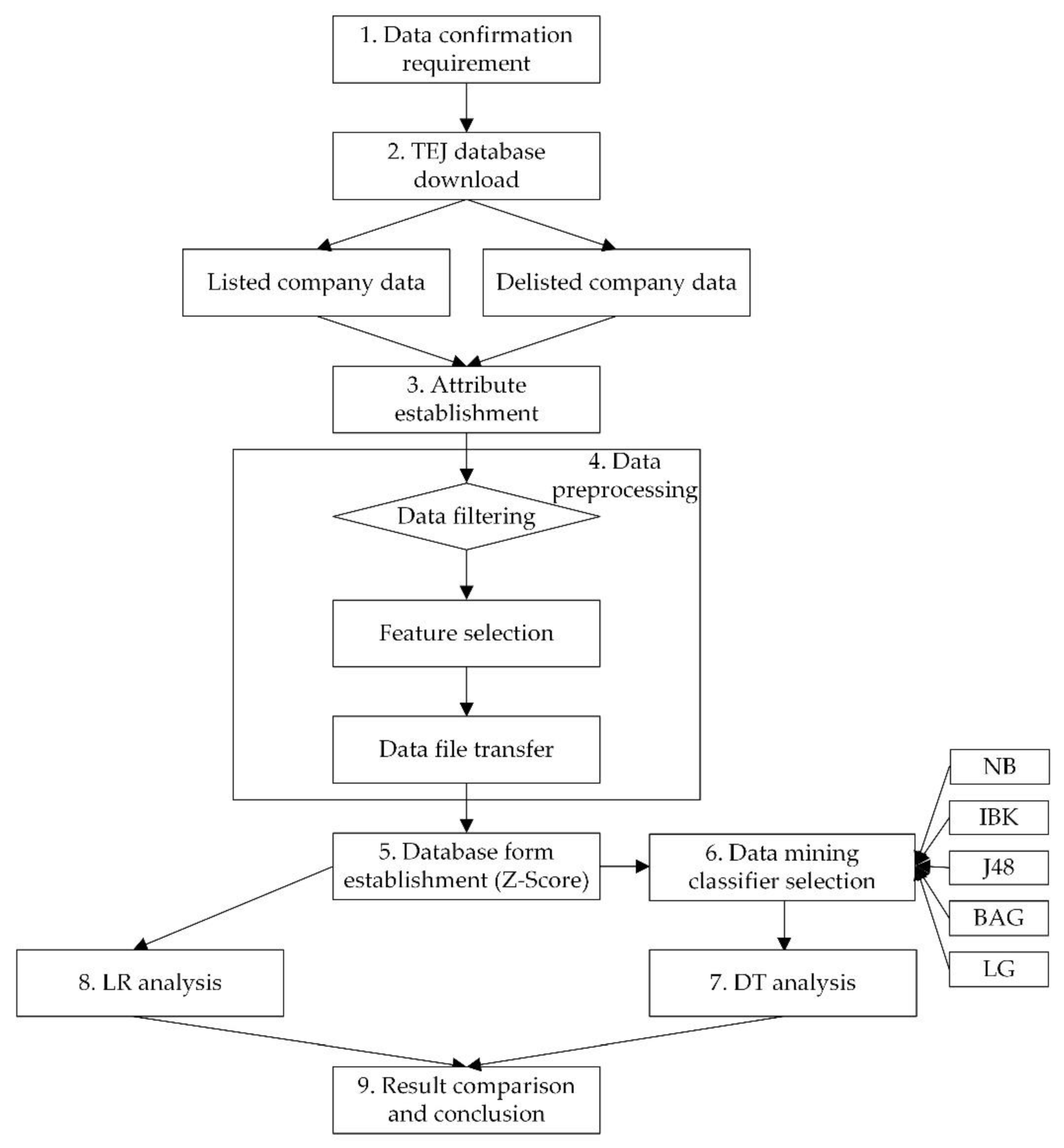
3.1. Research Framework

This study takes the data of listed and delisted companies in Taiwan’s electronics industry as the research samples. The research data come from the Taiwan Economic Journal (TEJ) financial database. The data of stock price and financial variables are obtained from the TEJ database, and the financial ratios of listed and delisted companies are from TEJ finance data. The research steps are described below; please refer to Figure 1 research framework for details of the nine main steps.

3.2. Research Steps for the Proposed Hybrid Model

The hybrid bankruptcy prediction model proposed in this study mainly includes the following nine key steps, and they are described in detail, step by step, as follows:
Step 1. Data confirmation requirement
The data of financial statements are listed in sequence according to the industry category of listed and delisted companies. After the financial statements are determined, a large amount—both in depth and breadth—of financial data is collected, and that data are confirmed by integrating the opinions and discussions of experts and scholars. This is an important work in the early stage of data research and excavation.
Step 2. TEJ database download
The financial ratios and related financial data of this study are all taken from the database of the TEJ financial website. The stock price is based on the stocktaking at the beginning and end of the quarter. The financial statements and stock price data of listed and delisted companies from 1 January 2000 to 31 December 2019 are downloaded from the TEJ database. According to their opinions from the industry experts and scholars, the research samples are selected from the database samples, filtered, and then preprocessed.
Step 3. Attribute establishment
According to experts’ opinions and scholars’ papers, 22 conditional attributes and one decisional attribute are selected and determined. From the perspective of financial analysis, the causes of enterprise bankruptcy can be summarized as follows: low repayment ability, weak profitability, poor asset development ability, and low operation ability, among which the most important performance indicator is profitability. This study selects three indicators of profitability and one indicator of repayment ability for analysis. Importantly, this step has five key points for features are identified below:
  • Attribute: Refers to the features of data, which may change with time. For example, the return rate, surplus, and loss of each company’s stock price will not be the same in different years, quarters, or different time points. The quarter attribute is a value, the return rate attribute is a symbol, and the value may be 10, 0.5, 0, etc. The two attribute values are distinguished as symbols or numbers.
  • Selection of conditional attributes: Based on the opinions of scholars and experts, 22 conditional attributes are mainly selected, including time, quarter, debt ratio, accounts receivable turnover, inventory turnover, fixed assets turnover, operating profit rate, return on operating assets, interest coverage ratio, interest expense ratio, total assets growth rate, total assets turnover, net value turnover, current liabilities, total assets, cash flow ratio, net value per share, cash flow per share, turnover per share, liquidity ratio, quick ratio, and earnings per share. In this study, the conditional attribute data types used in financial ratios include no-type data, range data, and set data, which are in free text and digital form. Because of the way financial ratios are used, most of them are in digital form.
  • Decision attribute: Normal or bankruptcy is the decisional attribute, and the variables are then selected and analyzed. This study has one decision attribute: listed or delisted. That is, the data type of decisional attribute is a category for Y/N corresponded to normal/bankruptcy in text format.
  • DT analysis: Each node through the tree graph is a financial ratio, and each branch is the analysis of the previous financial ratio, which will divide the direction of instruction into two or more blocks. The analysis process can filter the branches of the layer. When the filtering and segmentation can no longer be performed into a separate branch, the layering process is completed, and bankrupt or normal is finally identified in leaf.
  • Coding: The conditional attributes of financial ratios with their references for illustrating the chosen reason are represented by coding X1, X2, X3, …, and X22 in this study, as shown in Table 1. The decision attribute is coded as X23.
Step 4. Data preprocessing
There is a large amount of data collected, which need to be filtered, cleaned, and sorted before they can be applied to the model analysis. Data filtering and cleaning can delete incomplete, duplicate, and similar or the same value of conditional data, filter out invalid and no-feature data, and retain the attributes that have an impact on the accuracy, so as to achieve the characteristics of reducing the attribute space dimension, which can not only improve the accuracy of analysis results but also benefit the mining efficiency effectively. Three important features are defined as follows:
  • Data filtering. Includes the following substeps: (1) filtering, (2) merging fields, (3) verifying data correctness, (4) cleaning, and (5) checking the data features of conditional attributes, such as outliers.
  • Feature selection. Feature selection is mostly used in classifier and regression analysis, which is for the use of classification function in this study. It is used to search all possible combinations of all attributes in the dataset to find the best group of attributes. In this study, machine attribute selection is used as follows. The machine feature selection of the research data of 2455 listed companies and 491 delisted companies are resampled and carried out by two-class classification methods; they are listed and delisted.
  • Data file transfer. After the feature selection of five groups of models with different company ratios (i.e., 1:1 to 5:1) for further analysis of the processing data of the imbalanced class classification problem, the key attributes were identified and are shown in Table 2. From Table 2, the empirical results of five groups of different company ratios were used as experimental data, with each modeled and analyzed. Next, the data for the listed and delisted companies were targeted and processed, the above data were transferred to files, and then they were to be analyzed by the following LR analysis for the next step.
Step 5. Database form establishment
Subsequently, working capital, total assets, statutory surplus reserve, undistributed surplus, EBIT, general stock market value at the end of the quarter, total liabilities, net operating income are mainly used to calculate the Z value of the Z-score model. Through the Z-score model, 2455 listed companies with Z > 2.99 and 491 listed companies with Z < 1.8 are selected for further data analysis and classification. Then, 2455 listed companies and 491 bankrupt companies are divided into five groups: 491 listed companies to 491 bankrupt companies (1:1), 982 listed companies to 491 bankrupt companies (2:1), 1473 listed companies to 491 bankrupt companies (3:1), 1964 listed companies to 491 bankrupt companies (4:1), and 2455 listed companies to 491 bankrupt companies (5:1). The five groups achieved from various data partitioning rates were used for the two purposes of assessment to learn and gather relevant information about classification performance and research progress. One is in identifying determinants of influencing decisional attributes on different classifiers and hybrid models, and the other is to process the imbalanced class data problem to measure different performances.
Step 6. Data mining classifier selection
Afterwards, this study used five classifiers, which are widely used by financial bankruptcy researchers. NB, KNN, DT J48, BAG, and LG classifiers are used to evaluate the accuracy of the model in two types of proportion segmentation (seven proportions) and 10-fold cross-validation. The dataset collected from the database is divided into two subsets for training and testing in order to find the best prediction model or classifier.
Step 7. DT analysis
DT is a typical classifier of supervision type in the data mining field, which is usually used for prediction and modeling functions. Classifiers can help to analyze the huge amount of multidimensional data into some rules that are easy to understand. The elements of DT in this study include: (1) root refers to influence attribute, (2) branch is the classification method influencing attributes, and (3) leaf is the last to distinguish bankrupt and normal company; for example, Y is normal and N is bankrupt.
Step 8. LR analysis
In this study, logistic binary regression is set as listed or delisted, the variable is a dependent type (outcome variable), also known as an independent variable, which usually indicates the reason for speculation. Other attribute variables are dependent ones, also known as explanatory variables, which usually represent the results to be inferred. The data transferred from Step 4 are then analyzed by the LR model, and the results for the LR analysis will be used in a comparison study.
Step 9. Result comparison and conclusion
Finally, different data segmentation rates, different assessment methods, and different classifiers with hybrid models are compared for the varied purposes of measurement in this step. Thus, some comparison studies, empirical results, research findings, and study conclusions are made available in a unified approach.

4. Validation Analysis

This study collected the financial ratio data of listed and delisted companies from 2000 to 2019, selected listed and delisted companies using the Z-score model, used machine learning tools for big data applications to analyze the predictable bankruptcy attributes, and established a hybrid classification model to analyze the attributes and determinants in the following six parts.

4.1. Descriptive Statistics of the Attributes Used

It is a basic requirement to present information about the used dataset. First, only the related data for the datasets collected with 491 normal and 491 bankrupt companies displayed in Table 3 are used as an example for completely showing the original data information from 23 conditional and decisional attributes. Next, descriptive statistics, such as minimum, maximum, mean, and standard deviation are calculated for all of the variables (attributes) of the same segmentation 1:1 dataset, and their information is shown in Table 4 to portray the basic information about the attributes analyzed in the following experiments.

4.2. Data Mining Classifier Technology

In this study, all datasets for per share normal companies and bankrupt companies are divided into two categories and then analyzed using classification algorithms. The experiments are designed and run properly. Five classifiers, namely NB, LG, KNN (IBK algorithm), BAG, and DT (J48), are selected to build models for their past superiority in different application fields and find out the best prediction analysis attributes. The introduction mode of classifier evaluation performance adopts two methods of varied proportional segmentation and cross-validation. The DT is used to analyze and extract decisional rules of financial bankruptcy prediction. Afterwards, the LR model of statistical software is used in the analysis, and the influence score of attributes is then cross-verified and implemented with algorithm comparison. Subsequently, all the empirical results are aggregated in the next subsection for easy presentation and reading.

4.3. Empirical Analysis of Classifiers

The classifier prediction model uses the data from 2000 to 2019 to analyze the financial ratio of normal companies to those delisted due to financial bankruptcy three times. After selecting with unselected attributes, the company with normal or bankrupt decisions attributed in each quarter is given priority to implement and analyze with mining tools according to different classifiers to observe the performance of financial ratios. The same company is regarded as a different company to evaluate the performance in each quarter. After feature selection, the same financial ratio data is used to implement and analyze according to the same classifier by using cross-validation 10 times. Therefore, the five groups of different ratios of listed and delisted companies are highlighted in the following five directions and benefits (note that due to the limited space in this study, all of the following experiments only list the presentation of key data comparison).
1. For the ratio 1:1, 491 normal companies and 491 companies delisted due to financial bankruptcy in the study are cross verified after proportional division, then selected with no-features and feature selection and respectively analyzed with decision factors by using the two partitioning methods of classification; the experimental results for the ratio 1:1 are displayed into two key interests as below.
(1) Classifier analysis with no-feature selection is shown in Table 5. From Table 5, two key directions are addressed (note that the bold in figures is referred to a significant result):
(a) Analyze with different classifiers for training segmentation percentage 67—NB (97.84%), best LG (100%), IBK (91.05%), worst BAG (50%), J48 (99.69%).
(b) Cross-validation 10-fold attribute evaluation narrative—NB (98.27%), LG (98.78%), IBK (92.36%), worst BAG (50%), best J48 (99.8%).
From the above overall results in Table 5, it is interesting that DT J48 has the best classifier, and the LG is the second best regardless of training segmentation rate or cross-validation method.
(2) Classifier analysis with feature selection is shown in Table 6. From Table 6, two key points are addressed:
(a) Analyze with different classifiers for segmentation percentage 67—best NB (99.07%), LG (98.46%), worst IBK (97.84%), BAG (98.15%), worst J48 (97.84%).
(b) Cross-validation 10-fold attribute evaluation narrative—worst NB (98.37%), best LG (99.39%), IBK (98.98%), BAG (99.29%), J48 (99.19%).
From Table 6, it is clearly indicated that the classification accuracy for the five classifiers is increased after performing the feature selection technique, and the accuracy for all is over 97%. It is found that the feature selection has some benefits in stably improving different classifiers.
2. For the ratio 2:1, 982 normal companies and 491 companies delisted due to financial bankruptcy in the study are cross verified after proportional division, then selected with no-features and feature selection and analyzed with decision factors by using two partitioning methods of classification, respectively; the empirical results for the ratio 2:1 are represented by two main concerns. (1) Table 7 shows classifier analysis with no-feature selection for the ratio 2:1 of two partitioning methods. (2) Table 8 shows classifier analysis with feature selection for ratio 2:1. From Table 7, the two better classifiers are also LG and J48, but the IBK and BAG have good improvement after feature selection in Table 8, which is also an interesting concern for finding out the potential reason.
3. For the ratio 3:1, 1473 normal companies and 491 delisted companies are cross verified after proportional division, then selected with no-features and feature selection and analyzed with decision factors by using two partitioning methods of classification technique, respectively; their experimental results are described in terms of two interests. Table 9 lists classifier analysis with no-feature selection for the ratio 3:1, and Table 10 lists classifier analysis with feature selection. From Table 9, LG and J48 have better accuracy performance, and those of J48, BAG, and IBK are superior to the others in Table 10.
4. For the ratio 4:1, 1964 normal companies and 491 companies delisted due to financial bankruptcy in the study are cross verified after proportional division, then selected with no-features and feature selection and respectively analyzed with decision factors by using two partitioning methods of classification tools; the empirical results for the ratio 4:1 are aggregated into two core highlights. One is to show Table 11 for classifier analysis with no-feature selection for the ratio 4:1, the other is Table 12, to show classifier analysis with feature selection. From Table 11, it is obvious that LG has the best performance with no-feature selection in all partitioning methods, and J48 has the second-best performance. Regarding Table 12, it is also obvious that the LG also has the best performance in almost segmentation rate except for cross-validation 10-fold.
5. For the ratio 5:1, 2455 normal companies and 491 companies delisted due to financial bankruptcy in the study are cross verified after proportional division, then selected with no-features and feature selection and analyzed with decision factors by using two partitioning methods of classification technique, respectively; the experimental results for the ratio 5:1 are integrated into two main points. First, Table 13 highlights classifier analysis with no-feature selection for the ratio 5:1. Second, Table 14 displays classifier analysis with feature selection. It is also indicated that the LG and J48 have the two best performers in terms of accuracy with no-feature selection in Table 13; however, IBK and BAG show the best performance with feature selection in Table 14. This interesting phenomenon is valuable for addressing the issue of potential conflicts in a future study.

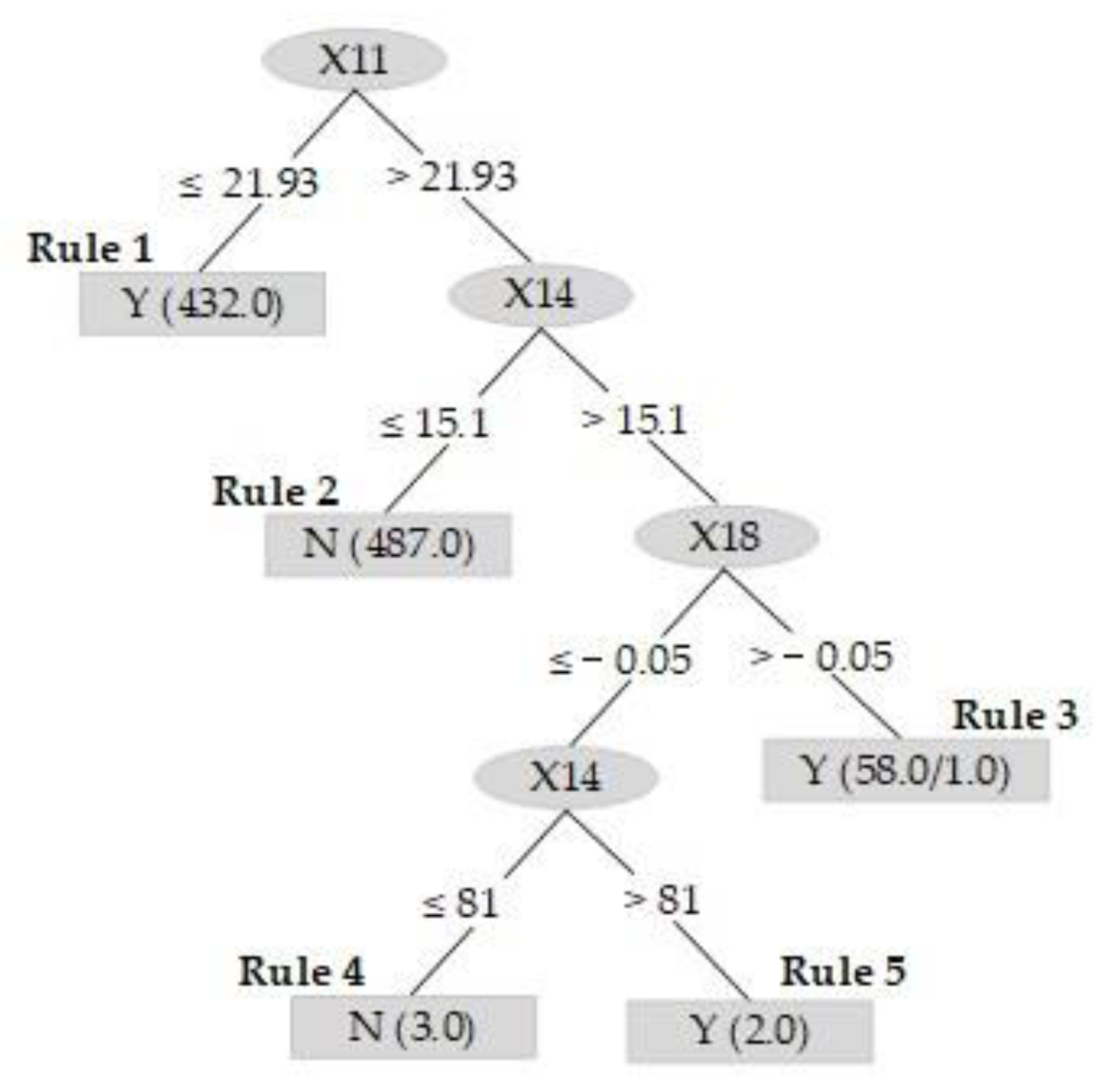
4.4. DT Empirical Analysis

After the empirical analysis for DT is implemented, the J48 classifier analysis shows that the effective attributes are X11 debt ratio, X14 fixed assets turnover, and X18 interest expense ratio. At the same time, the DT of the J48 classifier feature selection is shown in Figure 2. From Figure 2, whether 491 normal companies and 491 bankrupt companies (1:1) are bankrupt (N) or normal (Y), the DT (Figure 2) is as follows (note that due to ease presentation, examples are for only one bankrupt (N) and one normal (Y) case). The meaningful decision rules provide effective regulations for judging a normal or bankrupt company to interested parties; thus, its valuable outcomes are an important contribution in this study.
(1)
Rule 2: If X11 > 21.93, and X14 ≤ 15.1, then X23 → N.
Description: If the liquidity ratio is greater than 21.93 and the fixed assets turnover is less than or equal to 15.1, then it is a bankrupt company.
(2)
Rule 3: If X11 > 21.93, and X14 > 15.1, and X18 > −0.05, then X23 → Y.
Description: If the liquidity ratio is greater than 21.93, the fixed assets turnover is greater than 15.1, and the interest expense ratio is greater than −0.05, then it is a normal company.

4.5. LR Empirical Analysis

The LR experimental analysis is conducted into a quantitative measurement of five parts for the purpose of comparative studies with the classifiers used, and the empirical results of LR analysis are concluded in the next subsection for convenient reading.
First, the empirical process to establish binary LR analysis for the bankruptcy prediction model for addressing research data of the ratio 1:1 on 491 normal companies and 491 companies delisted due to comparative studies of financial bankruptcy is as follows:
  • The comprehensive model verification of 491 normal and 491 bankrupt companies (1:1) is identified as: (1) the mode of the ratio 1:1 has 1% and 5% significances, and (2) four (X2 quarter Q2, X9, X11, and X14) of the 22 variables effectively represent whether the occurrence of financial bankruptcy will affect the classification results.
  • After the feature selection of 491 normal and 491 bankrupt companies (1:1), the binary analysis of LR is determined: the model prediction accuracy of the ratio 1:1 is achieved 99.5%.
  • For the LR analysis result, Table 15 shows information that the dependent variable of LR reaches at least 5% significance for regression analysis of financial bankruptcy sample data.
Second, the empirical results to establish logistic binary financial bankruptcy prediction attribute model for research data of 982 normal companies and 491 companies delisted due to comparative studies of financial bankruptcy are as follows:
  • The comprehensive model verification of 982 normal and 491 bankrupt companies (2:1) is defined as (1) the mode of the ratio 2:1 has 1% significance, and (2) three (X9, X11, and X14) of the 20 variables effectively represent and predict whether the occurrence of financial bankruptcy will affect the classification results.
  • After the feature selection of 982 normal and 491 bankrupt companies (2:1), the model prediction accuracy achieves 99.3% for the binary analysis of LR.
  • For the LR analysis result, Table 16 shows information that the dependent variable of LR reaches 1% significance for regression analysis of financial bankruptcy sample data.
Third, the empirical results to establish logistic binary financial bankruptcy prediction attribute model for research data of 1473 normal companies and 491 companies delisted due to the above same reason of financial bankruptcy are as follows:
  • The comprehensive model verification of 1473 normal and 491 bankrupt companies (3:1) is identified as (1) the mode of the ratio 3:1 has at least 10% significance, and five (X9, X10, X11, X14, and X22) of the 20 variables effectively represent and predict whether the occurrence of financial bankruptcy will affect the classification results.
  • After the feature selection of 1473 normal and 491 bankrupt companies (3:1), the binary analysis of LR achieves the model prediction accuracy of 99.5%.
  • For the LR analysis result, Table 17 shows that the dependent variable of LR reaches at least 10% significance for regression analysis of financial bankruptcy sample data.
Fourth, the empirical results to establish logistic binary financial bankruptcy prediction attribute model for research data of 1964 normal companies and 491 companies delisted due to comparative studies of financial bankruptcy are as follows:
  • The comprehensive model verification of 1964 normal and 491 bankrupt companies (4:1) is focused on the two points: (1) the four to one mode has 1% significance, and five (X9, X10, X11, X14, and X22) of the 20 variables effectively also represent and predict whether the occurrence of financial bankruptcy will affect the classification results.
  • After the feature selection of 1964 normal and 491 bankrupt companies (4:1), the binary analysis of LR also achieves the model prediction accuracy of 99.5%.
  • For the LR analysis result, Table 18 shows that the dependent variable of LR reaches at least 10% significance for regression analysis of financial bankruptcy sample data.
Finally, the empirical results to establish logistic binary financial bankruptcy prediction attribute model for research data of 2455 normal companies and 491 companies delisted due to the same comparison benefit of financial bankruptcy are as follows:
  • The comprehensive model verification of 2455 normal and 491 bankrupt companies (5:1) is also defined as (1) the four to one mode has 1% significance, and (2) five (X6, X9, X11, X14, and X22) of the 20 variables effectively also represent and predict whether the occurrence of financial bankruptcy will affect the classification results.
  • After the feature selection of 2455 normal and 491 bankrupt companies (5:1), the binary analysis of LR is obtained the model prediction accuracy of 99.6%.
  • For the LR analysis result, Table 19 shows that the dependent variable of LR reaches at least 5% significance for regression analysis of financial bankruptcy sample data.

4.6. Result Comparison and Conclusion

From the above analytical results for classifiers, DT, and LR method, it is indicated that different classifiers or methods have different performances with different segmentation training/testing ratios after performing no-feature selection or the feature selection method, and the decisional rules in the tree-structure image are identified and extracted by DT, which can benefit instructionally meaningful knowledge to explicitly track the process of financial bankruptcy for interested parties. Table 20 shows the conclusive statistical results from Table 5, Table 7, Table 9, Table 11, Table 13, and Table 21 shows the same but for Table 6, Table 8, Table 10, Table 12, and Table 14. Table 22 also shows the statistical results of LR analysis for samples of the five ratio groups but for Table 15, Table 16, Table 17, Table 18 and Table 19. From the above results, four directions are identified. (1) From Table 20, it is indicated that in this study, the best classifiers according to rank are the LG and J48 algorithms for the data used by using the no-feature selection technique. (2) The best performance in terms of accuracy when performing feature selection is observed for LG and J48 concurrently, and then BAG, IBK, and NB according to ranking from Table 21. (3) Moreover, it is interesting that in cross-validation, the classification accuracy for BAG and IBK has significantly improved 10-fold after performing the feature selection method from the above tables; thus, it will be of value to explore the potential hidden reason for this interesting and consequential phenomenon in subsequent research. (4) It is observed from Table 22 that LR has a high average accuracy of 99.48%, and the significant determinants of X9, X11, and X14 are identified as influencing financial bankruptcy.

5. Discussions and Empirical Findings

By using the Altman model, 2455 normal and 491 bankrupt companies were selected and divided into groups of different ratios (491 normal and 491 bankrupt (1:1), 982 normal and 491 bankrupt (2:1), 1473 normal and 491 bankrupt (3:1), 1964 normal and 491 bankrupt (4:1), 2455 normal and 491 bankrupt (5:1)) for various classifiers and LR analysis. Through the empirical conclusion, this study obtains and discusses the results, with two kinds of research findings, management implications, and research limitations, which are described as follows.

5.1. Discussion of Empirical Results

The situation of the current COVID-19 pandemic has especially prompted studies on the issue of financial bankruptcy prediction; thus, it is an interesting topic for further discussion and exploration. Regarding the empirical results, three key points can be discussed. (1) It is of value and interest to discuss an appropriate classifier or hybrid model to address the particular problem of financial bankruptcy; thus, based on the given motivation, this study aims to establish a suitable model for the identification of financial bankruptcy. However, it is difficult to search for the best classifier or a suitable model to address the data topic of financial fields due to the variation in specific data characteristics and the diversity in classification techniques their accordance with each other, which are addressed in this study. (2) In past studies, it has been described that some classifiers have black-box attacks and associated limitations, and the results do not provide rule-guided knowledge; thus, it is impossible to support a white box for some classifiers, such as NB, LG, IBK algorithm of KNN, and BAG. Importantly, this study bridges this gap closely by employing the J48 algorithm of DT, and it provides decisional rules of law, which can be followed and learned and maps an observation to an appropriate action by interested parties. (3) In the comparison of the empirical results, the performance on components of the proposed hybrid model should be further discussed in the following four directions for future benefits. (a) Different groups of data segmentation partition can be differentiated using classification methods. (b) The performance with different training/testing ratios has the same problem. (c) Using or not using the feature selection method is a valuable issue to be measured. (d) Furthermore, for the BAG and IBK approaches, they have significantly increased (10-fold) performance in cross-validation when concurrently using the feature selection method. This interesting observation is also a valuable topic to further explore and discuss the possible consequences.

5.2. Research Findings of Classifiers

In this study, the attribute variables are brought into five analysis methods of NB classifier, KNN (IBK) classifier, DT J48 classifier, BAG classifier, and LG classifier for split validation rate, and 10-fold cross-validation is used to evaluate the model.
  • Company bankruptcy classifier assessment.
    (1) Score of company bankruptcy proportion segmentation: (a) the best feature selection is the 4:1 company model of LG classifier; (b) the best classifiers are DT J48 classifier (max 100%, min 99.10%) and LG classifier (max 100%, min 99.10%); (c) in the 5:1 company model, BAG classifier increases the most by 42.91%; (d) BAG classifier performs worst.
    (2) Evaluation of company bankruptcy cross-validation: (a) the best feature selection is three to one company model of KNN (IBK) classifier; (b) the classifiers with the best accuracy of 99.59% are KNN (IBK) classifier and DT J48 classifier; (c) BAG classifier increases the most by 49.52% in this model; (d) NB performs worst.
The significant attributes of each company proportion in the classifier analysis are shown in Table 23.

5.3. Research Findings of LR

The difference between logistic binary regression and linear regression is the degree of dependent variable results. When the dependent variable is classified into one of two categories (generally expressed as 1 or 0), logistic binary regression will be used; conversely, if the dependent variable is a continuous one, it will be analyzed by linear regression. Because each attribute selected in this study is significant, the LR analysis of no-feature selection will not have very significant attributes. Therefore, feature selection of attributes should be conducted using an analysis tool and then analyzed by LR. In the LR analysis of five models, the data with the most significant influence after feature selection is represented by the number of *, and the higher the number, the more significant it is, as shown in Table 24.

5.4. Managerial Implications

Modern enterprises focus attention on operating efficiency, how to make the company operate systematically, creating a prospective strategy for the company, and the way to make profits, in which correct management is implied. The operator not only needs to have the decision-making ability but also needs to have the ability to observe the financial ratio, so as to create more value for shareholders. Therefore, this study determines the optimal financial ratio for easily observing and providing managerial references for investors and managers. The biggest difference between senior managers and company operators is that the former should do their work correctly, and the latter must choose to implement the right strategy. If they have significant financial attributes, they can observe the changes in financial attributes in advance, then choose the right direction and reduce losses. This study selects five groups of different company ratios based on the financial indicators of financial early warning and focuses on the listed companies in Taiwan to identify the factors with highly significant attributes through the analysis of financial indicators, and to identify the significant financial attributes to detect the capability of companies in financial bankruptcy through attributes of feature selection (liquidity ratio (X9), debt ratio (X11), and fixed asset turnover (X14)), so as to give reference.

5.5. Research Limitations

This study provides some specific research limitations to identify gaps in research in the following three parts. First, the experimental datasets are extracted from the TEJ database, which is official information publicly published and recognized by government agencies. Thus, when using official company reports, there is a risk of receiving and using fraudulent data. A limitation of this study is that filtering out such data was not executed. Second, regarding the operating income of a financial ratio, its discounting or discount rate is not used and represents a limitation in this study because official information on this is published by government bodies, and discounts are not considered in the scope of the proposed hybrid model. Finally, this study also has limitations regarding the time span of data and data fraudulence.

6. Conclusions and Future Research

This study only focuses on the listed companies in Taiwan, using LR and classifier data mining to identify financial attributes that will affect the prediction. Through the results of empirical analysis, the conclusion of this study can be summarized according to the following aspects, as well as subsequent research details.

6.1. Conclusions

The empirical results can be summarized into the following three key points:
  • Proportional classifier features between financial bankruptcy and normal companies. After the feature selection of five ratio groups of companies using financial indicators, the main characteristics were found to be quarter (X2), net value per share (X6), liquidity ratio (X9), quick ratio (X10), debt ratio (X11), fixed assets turnover (X14), interest coverage ratio (X17), interest expense ratio (X18), and earnings per share (X22).
  • The research of company proportion has a significant impact on the financial bankruptcy early warning attribute classifier. In the financial early warning model of the five ratio groups of companies, the common significant variables of classifiers are: liquidity ratio (X9), quick ratio (X10), debt ratio (X11), fixed assets turnover (X14), interest expense ratio (X18), earnings per share (X22). In addition to the features of quarter (X2), net value per share (X6) and interest coverage ratio (X17) variables of 1:1, and 2:1 company ratios, other features have a significant relationship in the DT (J48) bankruptcy early warning model.
  • The research of five groups of different company ratios, combined with LR analysis and comparison. In this study, the difference in overall accuracy of the five ratio groups of companies is more than 99.3% in the single indicator financial early warning model. In other words, the highest error rate of LR and bankruptcy indicators of companies in financial bankruptcy is 0.7%. In the single indicator financial early warning model, the overall difference accuracy is more than 99.3%. Therefore, the models for the five ratio groups of companies can distinguish the financial ratio of the company in financial bankruptcy, but the regression analysis value for the sample data of the five groups does not have highly significant attributes. The possible reason is that all attributes have influence, so there is no significant parameter change. After feature selection of five groups of company proportion by classifier, the significant variables of LR analysis are liquidity ratio (X9), debt ratio (X11), fixed assets turnover (X14), and earnings per share (X22).
The results of this study show that financial ratios, with different ratios of companies and bankruptcy indicators, can accurately predict significant cases and feature attributes of financial bankruptcy. Therefore, analysis of financial bankruptcy attributes based on the feature financial ratio and a company ratio is more effective than using the early warning model of no-feature financial ratio. The common high significance attributes of the two analysis tools are debt ratio (X11) and fixed assets turnover (X14), which can also be used to better understand the influence of enterprises in terms of various financial data.

6.2. Future Research

Although this study has some benefits for defining the financial bankruptcy issue, there is still some space for improvement for subsequent research. Thus, eight routes can be addressed in subsequent research. (1) Financial bankruptcy does not solely occur in listed companies. Later, we can expand the sample with more public companies and find more research samples from the OTC market and the emerging OTC market so as to work out the same financial ratios from this study. (2) Different data extracted from a variety of industries can be used to test the performance of the proposed forecasting model. (3) Alternatives to using more financial ratios from other studies in the literature for testing the proposed hybrid model are needed. (4) More test data for different time periods than in this study can be used for further reverifying the study performance. (5) The inclusion of additional evaluation criteria is a requirement for further measuring the proposed model. (6) Other potential models can be organized with the proposed hybrid model to further measure and test the proposed model. (7) Current practitioners in Taiwan have no special rules for identifying the financial bankruptcy of a corporate, and this study cannot be considered complete given the time limitation, lack of data confidentiality, or the possibility of data fraudulence. Thus, it is expected that results from the future direction of research can supplement the prediction models of other classification methods aimed at addressing these shortfalls. (8) In future research, there is also room to study different countries or regions and explain the relevance of variables in early crisis warning research.
More importantly, the research data and attributes need to be remodeled and the proposed model retested to determine whether the research results can persist through the transition and be applied to various industries or countries when the results have changed. Afterwards, it is also expected that an effective suggestion with high accuracy will be provided to assist future interested parties in considering the aspect of financial bankruptcy and, even more so, in making significant commercial investment decisions.

Author Contributions

Conceptualization, Y.-S.C. and Q.-J.L.; methodology, Y.-S.C.; software, Q.-J.L.; visualization, C.-M.L. and Q.-J.L.; writing—original draft, Y.-S.C. and Q.-J.L.; writing—review and editing, Y.-S.C., C.-K.L., C.-M.L. and S.-F.C. All authors have read and agreed to the published version of the manuscript.

Funding

This research was partially supported by the Ministry of Science and Technology of Taiwan, grant numbers MOST 108-2410-H-146-001 and 109-2221-E-146-003.

Conflicts of Interest

The authors declare no conflict of interest.

References

  1. Zhang, Y.; Liu, R.; Heidari, A.A.; Wang, X.; Chen, Y.; Wang, M.; Chen, H. Towards augmented kernel extreme learning models for bankruptcy prediction: Algorithmic behavior and comprehensive analysis. Neurocomputing 2021, 430, 185–212. [Google Scholar] [CrossRef]
  2. Kou, G.; Xu, Y.; Peng, Y.; Shen, F.; Chen, Y.; Chang, K.; Kou, S. Bankruptcy prediction for SMEs using transactional data and two-stage multiobjective feature selection. Decis. Support. Syst. 2021, 140, 113429. [Google Scholar] [CrossRef]
  3. Du Jardin, P. Dynamic self-organizing feature map-based models applied to bankruptcy prediction. Decis. Support. Syst. 2021, 147, 113576. [Google Scholar] [CrossRef]
  4. Zhang, H.; Jiang, L.; Yu, L. Attribute and instance weighted naive Bayes. Pattern Recognit. 2021, 111, 107674. [Google Scholar] [CrossRef]
  5. Zhang, Z.; Han, Y. Detection of ovarian tumors in obstetric ultrasound imaging using logistic regression classifier with an advanced machine learning approach. IEEE Access 2020, 8, 44999–45008. [Google Scholar] [CrossRef]
  6. Kück, M.; Freitag, M. Forecasting of customer demands for production planning by local k-nearest neighbor models. Int. J. Prod. Econ. 2021, 231, 107837. [Google Scholar] [CrossRef]
  7. Sandag, G.A. A prediction model of company health using bagging classifier. JITK J. 2020, 6, 41–46. [Google Scholar] [CrossRef]
  8. Abspoel, M.; Escudero, D.; Volgushev, N. Secure training of decision trees with continuous attributes. Proc. Priv. Enhancing Technol. 2021, 2021, 167–187. [Google Scholar]
  9. Li, H.; Shu, L.; Yu, J.; Xian, Z.; Duan, H.; Shu, Q.; Ye, J. Using Z-score to optimize population-specific DDH screening: A retrospective study in Hangzhou, China. BMC. Musculoskelet. Disord. 2021, 22, 344. [Google Scholar]
  10. Sun, D.; Xu, J.; Wen, H.; Wang, D. Assessment of landslide susceptibility mapping based on Bayesian hyperparameter optimization: A comparison between logistic regression and random forest. Eng. Geol. 2021, 281, 105972. [Google Scholar] [CrossRef]
  11. Hopwood, T. Accounting as Social and Institutional Practice; Cambridge University Press: Cambridge, UK, 1994. [Google Scholar]
  12. Ashraf, S.; Félix, E.G.S.; Serrasqueiro, Z. Do traditional financial distress prediction models predict the early warning signs of financial distress? J. Risk Financ. Manag. 2019, 12, 55. [Google Scholar] [CrossRef] [Green Version]
  13. Jones, S.; Johnstone, D.; Wilson, R. Predicting corporate bankruptcy: An evaluation of alternative statistical frameworks. J. Bus. Financ. Account. 2017, 44, 3–34. [Google Scholar] [CrossRef]
  14. Jones, S.; Johnstone, D.; Wilson, R. An empirical evaluation of the performance of binary classifiers in the prediction of credit ratings changes. J. Bank. Financ. 2015, 56, 72–85. [Google Scholar] [CrossRef]
  15. Faris, H.; Abukhurma, R.; Almanaseer, W.; Saadeh, M.; Mora, A.M.; Castillo, P.A.; Aljarah, I. Improving financial bankruptcy prediction in a highly imbalanced class distribution using oversampling and ensemble learning: A case from the Spanish market. Prog. Artif. Intell. 2020, 9, 31–53. [Google Scholar] [CrossRef]
  16. Pelekh, U.; Khocha, N.; Holovchak, H. Financial statements as a management tool. Manag. Sci. Lett. 2020, 10, 197–208. [Google Scholar] [CrossRef]
  17. Aswar, K.; Wiguna, M.; Hariyani, E.; Ermawati, E. Quality of financial statements in Indonesian local governments: An empirical investigation. J. Asian Financ. Econ. Bus. 2021, 8, 993–999. [Google Scholar]
  18. Anan, E. Determinants fraudulent financial statements using the SCORE model on infrastructure sector companies in Indonesia. Ilomata Int. J. Tax Account. 2021, 2, 113–121. [Google Scholar] [CrossRef]
  19. Chen, Y.J.; Liou, W.C.; Chen, Y.M.; Wu, J.H. Fraud detection for financial statements of business groups. Int. J. Account. Inf. Syst. 2019, 32, 1–23. [Google Scholar] [CrossRef]
  20. Arya, A.; Nagar, N. Stewardship value of income statement classifications: An empirical examination. J. Account. Audit. Financ. 2021, 36, 56–80. [Google Scholar] [CrossRef]
  21. Razak, L.A. Value of relevance of other comprehensive income in listing companies in LQ 45 index. Psychology 2021, 58, 512–517. [Google Scholar]
  22. Albanese, C.; Crepey, S.; Hoskinson, R.; Saadeddine, B. XVA analysis from the balance sheet. Quant. Financ. 2021, 21, 99–123. [Google Scholar] [CrossRef]
  23. Debelle, G. The reserve bank of Australia’s policy actions and balance sheet. Econ. Anal. Policy 2020, 68, 285–295. [Google Scholar] [CrossRef] [PubMed]
  24. Prili, G.S.P. Effect of operrationg cash flows on the amount of dividends dividends towards the company. J. Contemp. Inf. Technol. Manag. Account. 2021, 2, 35–38. [Google Scholar]
  25. Anand, M.P.G.; Samba, V.; Kumar, M.S.V.S. A comparative study on cash flow statements of HDFC and SBI banks. Eur. J. Mol. Clin. Med. 2021, 7, 5089–5094. [Google Scholar]
  26. Hameedi, K.S.; Al-Fatlawi, Q.A.; Ali, M.N.; Almagtome, A.H. Financial performance reporting, IFRS implementation, and accounting information: Evidence from Iraqi banking sector. J. Asian Financ. Econ. Bus. 2021, 8, 1083–1094. [Google Scholar]
  27. Bradbury, M.E.; Scott, T. What accounting standards were the cause of enforcement actions following IFRS adoption? Account. Financ. 2021, 61, 2247–2268. [Google Scholar] [CrossRef]
  28. Amalia, S.; Fadjriah, N.E.; Nugraha, N.M. The influence of the financial ratio to the prevention of bankruptcy in cigarette manufacturing companies sub sector. Solid State Technol. 2020, 63, 4173–4182. [Google Scholar]
  29. Nugraha, N.M.; Puspitasari, D.M.; Amalia, S. The effect of financial ratio factors on the percentage of income increasing of automotive companies in Indonesia. Int. J. Psychosoc. Rehabil. 2020, 24, 2539–2545. [Google Scholar]
  30. Amalina, N.S.S.; Utami, H.; Suroija, N. The analysis the financial perfomance using financial ratio by the decree of the Indonesian minister for Soe. Agregat 2020, 4, 100–122. [Google Scholar]
  31. Kliestik, T.; Valaskova, K.; Lazaroiu, G.; Kovacova, M.; Vrbka, J. Remaining financially healthy and competitive: The role of financial predictors. J. Compet. 2020, 12, 74–92. [Google Scholar] [CrossRef]
  32. Hosaka, T. Bankruptcy prediction using imaged financial ratios and convolutional neural networks. Expert Syst. Appl. 2019, 117, 287–299. [Google Scholar] [CrossRef]
  33. Ibrahim, I.; Abdulazeez, A. The role of machine learning algorithms for diagnosing diseases. J. Appl. Sci. Technol. Trends 2021, 2, 10–19. [Google Scholar] [CrossRef]
  34. Jacobs, M.; Pradier, M.F.; McCoy, T.H.; Perlis, R.H.; Doshi-Velez, F.; Gajos, K.Z. How machine-learning recommendations influence clinician treatment selections: The example of the antidepressant selection. Transl. Psychiatry 2021, 11, 1–9. [Google Scholar] [CrossRef]
  35. Goh, G.D.; Sing, S.L.; Yeong, W.Y. A review on machine learning in 3D printing: Applications, potential, and challenges. Artif. Intell. Rev. 2021, 54, 63–94. [Google Scholar] [CrossRef]
  36. Ageed, Z.S.; Zeebaree, S.R.; Sadeeq, M.M.; Kak, S.F.; Yahia, H.S.; Mahmood, M.R.; Ibrahim, I.M. Comprehensive survey of big data mining approaches in cloud systems. Qubahan Acad. J. 2021, 1, 29–38. [Google Scholar] [CrossRef]
  37. Espadinha-Cruz, P.; Godina, R.; Rodrigues, E.M. A review of data mining applications in semiconductor manufacturing. Processes 2021, 9, 305. [Google Scholar] [CrossRef]
  38. Savaglio, C.; Fortino, G. A simulation-driven methodology for IoT data mining based on edge computing. ACM Trans. Internet Technol. 2021, 21, 1–22. [Google Scholar] [CrossRef]
  39. Song, X.F.; Zhang, Y.; Gong, D.W.; Sun, X.Y. Feature selection using bare-bones particle swarm optimization with mutual information. Pattern Recognit. 2021, 112, 107804. [Google Scholar] [CrossRef]
  40. Omuya, E.O.; Okeyo, G.O.; Kimwele, M.W. Feature selection for classification using principal component analysis and information gain. Expert Syst. Appl. 2021, 174, 114765. [Google Scholar] [CrossRef]
  41. Hussain, K.; Neggaz, N.; Zhu, W.; Houssein, E.H. An efficient hybrid sine-cosine Harris hawks optimization for low and high-dimensional feature selection. Expert Syst. Appl. 2021, 176, 114778. [Google Scholar] [CrossRef]
  42. Fang, S.; Cai, Z.; Sun, W.; Liu, A.; Liu, F.; Liang, Z.; Wang, G. Feature selection method based on class discriminative degree for intelligent medical diagnosis. Comput. Mater. Contin. 2018, 55, 419–433. [Google Scholar]
  43. Covington, L.; Armstrong, B.; Trude, A.C.; Black, M.M. Longitudinal associations among diet quality, physical activity and sleep onset consistency with body mass index Z-Score among toddlers in low-income families. Ann. Behav. Med. 2021, 55, 653–664. [Google Scholar] [CrossRef] [PubMed]
  44. Pérez-Elvira, R.; Oltra-Cucarella, J.; Carrobles, J.A.; Teodoru, M.; Bacila, C.; Neamtu, B. Individual alpha peak frequency, an important biomarker for live z-score training neurofeedback in adolescents with learning disabilities. Brain Sci. 2021, 11, 167. [Google Scholar] [CrossRef]
  45. Nathan, K.; Livnat, G.; Feraru, L.; Pillar, G. Improvement in BMI z-score following adenotonsillectomy in adolescents aged 12–18 years: A retrospective cohort study. BMC Pediatr. 2021, 21, 184. [Google Scholar] [CrossRef]
  46. Lepetit, L.; Strobel, F.; Tran, T.H. An alternative Z-score measure for downside bank insolvency risk. Appl. Econ. Lett. 2021, 28, 137–142. [Google Scholar] [CrossRef]
  47. Dallaire, F. Z score disease or coronary artery disease: The (missing) link between statistics and anatomy in Kawasaki disease. J. Am. Soc. Echocardiogr. 2021, 34, 673–675. [Google Scholar] [CrossRef]
  48. Swalih, M.; Adarsh, K.; Sulphey, M. A study on the financial soundness of Indian automobile industries using Altman Z-Score. Accounting 2021, 7, 295–298. [Google Scholar] [CrossRef]
  49. Altman, E.I. Financial ratios, discriminant analysis and the prediction of corporate bankruptcy. J. Financ. 1968, 23, 589–609. [Google Scholar] [CrossRef]
  50. Khajenezhad, A.; Bashiri, M.A.; Beigy, H. A distributed density estimation algorithm and its application to naive Bayes classification. Appl. Soft Comput. 2021, 98, 106837. [Google Scholar] [CrossRef]
  51. Wang, Z.; Huang, S.; Wang, J.; Sulaj, D.; Hao, W.; Kuang, A. Risk factors affecting crash injury severity for different groups of e-bike riders: A classification tree-based logistic regression model. J. Saf. Res. 2021, 76, 176–183. [Google Scholar] [CrossRef]
  52. García, J.; Maureira, C. A KNN quantum cuckoo search algorithm applied to the multidimensional knapsack problem. Appl. Soft Comput. 2021, 102, 107077. [Google Scholar] [CrossRef]
  53. Mosavi, A.; Hosseini, F.S.; Choubin, B.; Goodarzi, M.; Dineva, A.A.; Sardooi, E.R. Ensemble boosting and bagging based machine learning models for groundwater potential prediction. Water Resour. Manag. 2021, 35, 23–37. [Google Scholar] [CrossRef]
  54. Rungskunroch, P.; Jack, A.; Kaewunruen, S. Benchmarking on railway safety performance using Bayesian inference, decision tree and petri-net techniques based on long-term accidental data sets. Reliab. Eng. Syst. Saf. 2021, 213, 107684. [Google Scholar] [CrossRef]
  55. Ohlson, J.A. Financial ratios and the probabilistic prediction of bankruptcy. J. Account. Res. 1980, 18, 109–131. [Google Scholar] [CrossRef] [Green Version]
  56. Szpulak, A. Assessing the financial distress risk of companies operating under conditions of a negative cash conversion cycle. e-Finans. Financ. Internet Q. 2016, 12, 72–82. [Google Scholar] [CrossRef] [Green Version]
  57. Berishvili, V. Industry average financial ratios for Georgia. Ecoforum J. 2020, 9, 1–6. [Google Scholar]
  58. Tsai, J.K.; Hung, C.H. Improving AdaBoost classifier to predict enterprise performance after COVID-19. Mathematics 2021, 9, 2215. [Google Scholar] [CrossRef]
  59. Alshehri, D.A.; Tayachi, T. Assets-liability management: A comparative study of national commercial bank and national bank of Kuwait. J. Arch. Egyptol. 2021, 18, 383–391. [Google Scholar]
  60. Almuhaya, R.M.; Hakim, S. Yemen banks during turmoil: An analytical study. J. Arch. Egyptol. 2021, 18, 1084–1095. [Google Scholar]
  61. Liu, Z.; Zhu, J. Research on financial risks of internet listed companies. J. Appl. Sci. Eng. 2021, 8, 13–17. [Google Scholar]
  62. Hsieh, T.Y.; Wang, M.H. Finding critical financial ratios for Taiwan’s property development firms in recession. Logist. Inf. Manag. 2001, 14, 401–413. [Google Scholar] [CrossRef]
Figure 1. Research framework of the proposed hybrid model step by step.
Mathematics 09 02622 g001
Figure 2. Feature selection DT for 491 normal and 491 bankrupt companies (1:1).
Mathematics 09 02622 g002
Table 1. Conditional attribute data type and information.
No.Conditional AttributeReferenceData TypeData ModelDecimal DigitCode
1TimeBy expertSyntax dataNominal-X1
2QuarterBy expertSyntax dataNominal-X2
3Current liabilities[56]Range dataNumber0X3
4Total assets[57]Range dataNumber0X4
5Cash flow ratio[56]Range dataNumber2X5
6Net value per share[58]Range dataNumber2X6
7Cash flow per share[56]Range dataNumber2X7
8Turnover per share[56]Range dataNumber2X8
9Liquidity ratio[56]Range dataNumber2X9
10Quick ratio[57]Range dataNumber2X10
11Debt ratio[56]Range dataNumber2X11
12Accounts receivable turnover[56]Range dataNumber2X12
13Inventory turnover[58]Range dataNumber2X13
14Fixed assets turnover[57]Range dataNumber2X14
15Operating profit rate[57]Range dataNumber2X15
16Return on operating assets[59]Range dataNumber2X16
17Interest coverage ratio[58]Range dataNumber2X17
18Interest expense ratio[60]Range dataNumber2X18
19Total assets growth rate[61]Range dataNumber2X19
20Total assets turnover[61]Range dataNumber2X20
21Net value turnover[62]Range dataNumber2X21
22Earnings per share[61]Set dataNumber2X22
Table 2. Feature selection attributes.
Normal vs. Bankrupt CompanyKey Attributes
491 vs. 491
(1:1)
Five attributes: X2 quarter, X9 liquidity ratio, X11 debt ratio, X14 fixed assets turnover, X18 interest expense ratio
982 vs. 491
(2:1)
Four attributes: X9 liquidity ratio, X11 debt ratio, X14 fixed assets turnover, X18 interest expense ratio
1473 vs. 491
(3:1)
Eight attributes: X6 net value per share, X9 liquidity ratio, X10 quick ratio, X11 debt ratio, X14 fixed assets turnover, X17 interest coverage ratio, X18 interest expense ratio, X22 earnings per share
1964 vs. 491
(4:1)
Eight attributes: X6 net value per share, X9 liquidity ratio, X10 quick ratio, X11 debt ratio, X14 fixed assets turnover, X17 interest coverage ratio, X18 interest expense ratio, X22 earnings per share
2455 vs. 491
(5:1)
Eight attributes: X6 net value per share, X9 liquidity ratio, X10 quick ratio, X11 debt ratio, X14 fixed assets turnover, X17 interest coverage ratio, X18 interest expense ratio, X22 earnings per share
Table 3. Information of the original data related for 491 normal and 491 bankrupt companies.
X1X2X3X4X5X19X20X21X22X23
2013/6/28Q284,839,54398,239,3744.44−10.820.4615.880.09Y
2013/9/30Q382,018,02493,777,3789.97−8.060.4711.810.17Y
2013/3/29Q183,159,54794,807,457−1.76−13.30.3616.560.02Y
2010/3/31Q1258,739868,14811.47−2.20.942.73−0.22Y
2011/3/31Q128,554,97150,463,6499.86252.472.196.2511.02Y
2013/6/28Q2289,0622,018,81580.611.970.540.610.63N
2008/6/30Q21,336,8894,949,06832.218.690.921.330.19N
2011/3/31Q1971,8205,879,43019.261.760.370.460.67N
2003/12/31Q42,018,55510,347,52150.0828.230.480.761.03N
2012/12/28Q41,153,1633,720,31338.092.940.681.032.79N
Table 4. Information of descriptive statistics for the 491 normal and 491 bankrupt companies.
AttributesData ModelMinimumMaximumMeanStandard Deviation
X1Nominal----
X2Nominal----
X3Numeric150,348.00356,161,801.0014,754,790.58429,752,491.600
X4Numeric194,701.00726,296,593.0038,310,531.31874,090,653.057
X5Numeric−117.69357.6424.18448.700
X6Numeric−13.21942.2531.34057.366
X7Numeric−40.72217.995.03015.858
X8Numeric0.37936.8057.25282.989
X9Numeric12.161078.33189.426140.629
X10Numeric2.19936.51137.504125.855
X11Numeric8.06209.2549.32720.295
X12Numeric1.36464.2614.03140.104
X13Numeric0493.2110.28421.734
X14Numeric0.221418.9837.528117.762
X15Numeric−155.2260.091.18922.718
X16Numeric−78.9592.167.51117.792
X17Numeric−122.399,719,988.3317,200.150315,301.953
X18Numeric−41,274.561730.09−42.2401321.687
X19Numeric−80.63281.5314.48735.509
X20Numeric0.137.481.4011.383
X21Numeric−1004.78277.772.30036.189
X22Numeric−18.63210.703.97614.287
Table 5. The classifier accuracy of no-feature selection for 491 normal and 491 bankrupt companies (1:1).
ClassifierSegmentation 65%Segmentation 67%Segmentation 70%Segmentation 75%Segmentation 80%Segmentation 85%Segmentation 90%Cross-Validation 10 Times
NB98.26%97.84%97.63%97.14%97.45%97.96%98.98%98.27%
LG98.84%100.00%99.66%99.59%100.00%99.32%100.00%98.78%
IBK89.83%91.05%91.19%90.61%90.31%91.84%94.90%92.36%
BAG50.00%50.00%48.81%51.02%44.90%40.82%40.82%50.00%
J4899.71%99.69%99.66%100.00%100.00%100.00%100.00%99.80%
Table 6. The classifier accuracy of feature selection for 491 normal and 491 bankrupt companies (1:1).
ClassifierSegmentation 65%Segmentation 67%Segmentation 70%Segmentation 75%Segmentation 80%Segmentation 85%Segmentation 90%Cross-Validation 10 Times
NB98.55%99.07%98.98%98.78%98.47%98.64%97.96%98.37%
LG98.55%98.46%98.64%98.37%98.47%99.32%98.98%99.39%
IBK97.67%97.84%97.29%97.14%98.47%98.64%97.96%98.98%
BAG97.97%98.15%97.97%98.37%99.49%99.32%100.00%99.29%
J4897.97%97.84%99.32%99.18%98.98%98.64%98.98%99.19%
Table 7. The classifier accuracy of no-feature selection for 982 normal and 491 bankrupt companies (2:1).
ClassifierSegmentation 65%Segmentation 67%Segmentation 70%Segmentation 75%Segmentation 80%Segmentation 85%Segmentation 90%Cross-Validation 10 Times
NB97.29%97.12%97.51%97.55%96.95%96.83%96.60%97.42%
LG99.22%99.79%99.32%100.00%99.32%99.10%100.00%99.80%
IBK93.41%93.21%92.99%92.39%92.54%95.48%95.92%94.03%
BAG65.12%65.23%65.61%65.22%66.10%66.97%63.95%66.67%
J4899.61%99.59%99.55%99.46%99.32%99.10%98.64%99.39%
Table 8. The classifier accuracy of feature selection for 982 normal and 491 bankrupt companies (2:1).
ClassifierSegmentation 65%Segmentation 67%Segmentation 70%Segmentation 75%Segmentation 80%Segmentation 85%Segmentation 90%Cross-Validation 10 Times
NB97.87%97.94%97.51%97.28%96.61%96.83%97.28%98.17%
LG99.42%99.59%99.55%99.46%99.32%99.10%99.32%99.12%
IBK98.45%98.35%98.42%98.10%98.31%99.10%98.64%99.25%
BAG99.22%99.38%99.10%98.91%99.32%99.10%99.32%99.52%
J4899.61%99.59%99.55%99.46%98.98%99.10%98.64%99.39%
Table 9. The classifier accuracy of no-feature selection for 1473 normal and 491 bankrupt companies (3:1).
ClassifierSegmentation 65%Segmentation 67%Segmentation 70%Segmentation 75%Segmentation 80%Segmentation 85%Segmentation 90%Cross-Validation 10 Times
NB95.92%95.99%95.76%95.93%95.42%94.92%94.90%96.44%
LG99.71%99.69%99.66%99.59%100.00%99.66%99.49%99.54%
IBK95.05%94.91%95.25%95.52%94.40%94.92%94.90%95.62%
BAG75.84%75.93%76.06%75.36%75.32%74.92%73.98%75.00%
J4898.25%98.30%99.15%99.80%100.00%99.32%100.00%99.54%
Table 10. The classifier accuracy of feature selection for 1473 normal and 491 bankrupt companies (3:1).
ClassifierSegmentation 65%Segmentation 67%Segmentation 70%Segmentation 75%Segmentation 80%Segmentation 85%Segmentation 90%Cross-Validation 10 Times
NB95.49%95.52%95.42%95.72%95.42%95.25%94.39%96.38%
LG98.98%98.92%98.81%98.57%98.98%98.64%99.49%99.34%
IBK99.13%99.23%99.32%99.19%99.49%99.32%98.98%99.64%
BAG99.13%98.92%99.49%99.39%98.98%99.32%99.49%99.39%
J4899.13%99.07%99.49%99.59%99.75%99.32%99.49%99.39%
Table 11. The classifier accuracy of no-feature selection for 1964 normal and 491 bankrupt companies (4:1).
ClassifierSegmentation 65%Segmentation 67%Segmentation 70%Segmentation 75%Segmentation 80%Segmentation 85%Segmentation 90%Cross-Validation 10 Times
NB95.46%94.94%95.38%95.28%95.11%96.20%95.92%94.83%
LG99.88%99.75%99.73%99.51%99.80%99.46%99.59%99.71%
IBK95.58%95.31%95.65%95.28%95.72%96.74%96.73%96.17%
BAG79.98%80.00%79.62%78.66%77.60%78.26%75.92%80.00%
J4898.60%98.52%99.59%99.51%99.39%99.18%98.78%99.59%
Table 12. The classifier accuracy of feature selection for 1964 normal and 491 bankrupt companies (4:1).
ClassifierSegmentation 65%Segmentation 67%Segmentation 70%Segmentation 75%Segmentation 80%Segmentation 85%Segmentation 90%Cross-Validation 10 Times
NB94.06%94.20%94.43%94.95%94.50%94.57%93.88%95.03%
LG99.77%100.00%99.86%99.84%99.80%99.73%99.59%99.39%
IBK99.42%99.38%99.46%99.51%99.39%99.46%99.18%99.59%
BAG98.60%98.52%99.46%99.02%99.39%97.83%98.78%99.51%
J4899.42%99.38%99.46%99.35%99.19%98.91%98.37%99.35%
Table 13. The classifier accuracy of no-feature selection for 2455 normal and 491 bankrupt companies (5:1).
ClassifierSegmentation 65%Segmentation 67%Segmentation 70%Segmentation 75%Segmentation 80%Segmentation 85%Segmentation 90%Cross-Validation 10 Times
NB94.96%93.93%92.31%91.85%92.36%93.21%92.54%91.96%
LG99.71%99.69%99.66%99.46%99.83%99.77%100.00%99.83%
IBK95.93%96.60%96.61%96.74%96.60%96.15%96.27%96.78%
BAG82.35%82.51%82.13%82.34%82.51%82.81%83.73%83.33%
J4899.42%99.90%99.89%99.73%99.66%99.55%98.98%99.73%
Table 14. The classifier accuracy of feature selection for 2455 normal and 491 bankrupt companies (5:1).
ClassifierSegmentation 65%Segmentation 67%Segmentation 70%Segmentation 75%Segmentation 80%Segmentation 85%Segmentation 90%Cross-Validation 10 Times
NB96.02%95.68%93.67%94.29%93.89%93.21%94.92%93.99%
LG99.32%99.28%99.32%99.18%98.98%99.32%99.66%99.52%
IBK99.32%99.59%99.43%99.59%99.49%99.55%100.00%99.59%
BAG99.03%99.49%99.66%99.59%99.32%99.55%100.00%99.46%
J4899.22%99.59%99.66%99.59%99.32%99.32%98.98%99.59%
Table 15. Significance values of feature selection variables of 491 normal and 491 bankrupt companies (1:1) in LR.
VariablesEstimate of BS.E.WaldSignificanceExp(B)
X2 quarter Q1 5.1900.158
X2 quarter Q2−5.7492.5515.0790.024 **0.003
X2 quarter Q3−1.7054.2660.1600.6890.182
X2 quarter Q4−2.1422.1910.9560.3280.117
X9 liquidity ratio0.0250.0115.8530.016 **1.026
X11 debt ratio−0.3230.1089.0150.003 ***0.724
X14 fixed assets turnover0.3300.10110.6890.001 ***1.391
X18 interest expense ratio0.0070.0090.6430.4231.007
Constant0.3493.9490.0080.9301.418
Note: it is ** when the significance reaches 5%, *** when 1%.
Table 16. Parameter values of feature selection variables of 982 normal and 491 bankrupt companies (2:1) in LR.
VariablesEstimate of BS.E.WaldSignificanceExp(B)
X9 liquidity ratio0.0130.00411.3170.001 ***1.013
X11 debt ratio−0.2340.03936.5900.000 ***0.792
X14 fixed assets turnover0.2690.03655.0770.000 ***1.308
X18 interest expense ratio−0.0020.0040.1950.6590.998
Constant2.5611.7892.0490.15212.944
Note: it is *** when the significance reaches 1%.
Table 17. Significance values of feature selection variables of 1473 normal and 491 bankrupt companies (3:1) in LR.
VariablesEstimate of BS.E.WaldSignificanceExp(B)
X6 net value per share−0.0250.0310.6250.4290.976
X9 liquidity ratio0.0400.0157.4060.007 ***1.041
X10 quick ratio−0.0280.0153.4020.065 *0.973
X11 debt ratio−0.2580.04435.0670.000 ***0.773
X14 fixed assets turnover0.2710.04142.7250.000 ***1.312
X17 interest coverage ratio0.0000.0000.0000.9831.000
X18 interest expense ratio−0.0020.0060.1070.7440.998
X22 earnings per share1.4710.27728.2610.000 ***4.354
Constant2.0991.8851.2400.2658.157
Note: it is * when the significance reaches 10%, *** when 1%.
Table 18. Significance values of feature selection variables of 1964 normal and 491 bankrupt companies (4:1) in LR.
VariablesEstimate of BS.E.WaldSignificanceExp(B)
X6 net value per share−0.0370.0252.1640.1410.963
X9 liquidity ratio0.0380.0129.9220.002 ***1.039
X10 quick ratio−0.0260.0124.5000.034 *0.974
X11 debt ratio−0.2530.03650.6450.000 ***0.776
X14 fixed assets turnover0.2750.03754.7810.000 ***1.317
X17 interest coverage ratio0.0000.0000.0350.8521.000
X18 interest expense ratio0.0030.0030.7510.3861.003
X22 earnings per share1.4910.25334.7710.000 ***4.443
Constant3.0601.6513.4340.06421.336
Note: it is * when the significance reaches 10%, *** when 1%.
Table 19. Significance values of feature selection variables of 2455 normal and 491 bankrupt companies (5:1) in LR.
VariablesEstimate of BS.E.WaldSignificanceExp(B)
X6 net value per share−0.0520.0254.5640.033 **0.949
X9 liquidity ratio0.0350.0119.3190.002 ***1.035
X10 quick ratio−0.0220.0123.3130.0690.979
X11 debt ratio−0.2650.03556.2280.000 ***0.767
X14 fixed assets turnover 0.2940.03956.1440.000 ***1.341
X17 interest coverage ratio000.0020.9651
X18 interest expense ratio0.0020.0040.4410.5071.002
X22 earnings per share1.7040.26242.4460.000 ***5.499
Constant4.0851.6765.9430.015 **59.439
Note: it is ** when the significance reaches 5%, and *** when 1%.
Table 20. The statistical results of best classifier for samples in the five ratio groups with no-feature selection from Table 5, Table 7, Table 9, Table 11, and Table 13.
ClassifierSegmentation 65%Segmentation 67%Segmentation 70%Segmentation 75%Segmentation 80%Segmentation 85%Segmentation 90%Cross-Validation 10 TimesCount
NB000000000
LG3432544429 1
IBK000000000
BAG000000000
J482134322219
1 The shading indicates the cases with better performance.
Table 21. The statistical results of best classifier for samples in the five ratio groups with feature selection from Table 6, Table 8, Table 10, Table 12, and Table 14.
ClassifierSegmentation 65%Segmentation 67%Segmentation 70%Segmentation 75%Segmentation 80%Segmentation 85%Segmentation 90%Cross-Validation 10 TimesCount
NB110000002
LG3222233118
IBK2201131212
BAG1021244216
J482334121218
Table 22. The statistical results of LR analysis of samples in the five ratio groups from Table 15, Table 16, Table 17, Table 18 and Table 19.
Ratio1:12:13:14:15:1Concern
Accuracy99.5%99.3%99.5%99.5%99.6%99.48%
DeterminantsX2: quarter Q2, X9, X11, X14X9, X11, X14X9, X10, X11, X14, X22X9, X10, X11, X14, X22X6, X9, X11, X14, X22X9, X11, X14
Table 23. Results of DT analysis for normal vs. bankrupt.
CodeConditional Attribute491 and 491 (1:1)982 and 491 (2:1)1473 and 491 (3:1)1964 and 491 (4:1)2455 and 491 (5:1)
X9Liquidity ratio SignificantSignificantSignificantSignificant
X10Quick ratio SignificantSignificant
X11Debt ratioSignificantSignificantSignificantSignificantSignificant
X14Fixed assets turnoverSignificantSignificantSignificantSignificantSignificant
X18Interest expense ratioSignificantSignificantSignificantSignificantSignificant
X22Earnings per share SignificantSignificantSignificant
Table 24. Statistics of logistic analysis results for normal vs. bankrupt.
No.Attributes491 and 491 (1:1)982 and 491 (2:1)1473 and 491 (3:1)1964 and 491 (4:1)2455 and 491 (5:1)Number of *
X2Quarter Q2** 2
X5Cash flow ration
X6Net value per share **2
X7Cash flow per share
X8Turnover per share
X9Liquidity ratio ** ********* *** 14
X10Quick ratio **
X11Debt ratio***************15
X12Accounts receivable turnover
X13Inventory turnover
X14Fixed assets turnover***************15
X15Operating profit rate
X16Return on operating assets
X17Interest coverage ratio
X18Interest expense ratio
X19Total assets growth rate
X20Total assets turnover
X21Net value turnover
X22Earnings per share *********9
Publisher’s Note: MDPI stays neutral with regard to jurisdictional claims in published maps and institutional affiliations.

