Entropy Optimization of First-Grade Viscoelastic Nanofluid Flow over a Stretching Sheet by Using Classical Keller-Box Scheme

Abstract

Nanofluids have better surface stability, thermal absorption, and distribution capacities are produced as heat transfer fluids. In current nanofluid-transport studies, together with the heat transfer mechanisms, entropy reduction in thermo- and non-Newtonian nanofluid models with changing thermophysical characteristics is heavily addressed. The entropy production is examined as thermodynamically stable first-grade viscoelastic nanofluid (FGVNF) flow over a flat penetrable, porous barrier. The uniform porous horizontal stretching of the surface in a Darcy type of pore media results in a fluid motion disturbance. In addition, this study also includes the effects of thermal radiation, viscous dissipation, and slip conditions at the border. Under boundary layer flow and Rosseland approximations, the governing mathematical equations defining the physical features of the FGVNF flow and heat transfer models are summarized. The governing nonlinear partial differential equation is transformed by similarity variables to achieve solutions in nonlinear ordinary differential equations. Approximative solutions for reduced ordinary differential equations are obtained by the Keller Box Scheme. Two distinct types of nanofluids, Copper-Engine Oil (Cu-EO) and Zirconium Dioxide-Engine Oil (ZrO₂-EO), are considered in this research. The graphs are produced to examine the effects of the different physical factors for the speed, temperature, and entropy distributions. The significant findings of this study are that the critical characteristics of (boundary layer) BL collectively promote temperature variation, including slip speed, diverse thermal conductivity, and non-Newtonian first-grade viscoelastic nanofluid, the concentration of nanoparticles as well as thermal radiation, and a high porous media. The other noteworthy observation of this study demonstrates that the (Cu-EO) FGVNF is a better conductor than (ZrO₂-EO) FGVNF transmission. The entropy of the system grows the Deborah number and volume fraction parameter.

1. Introduction

Boundary layer survey has significant benefits in figuring out the main concept behind transport phenomena through a fluid flow. The boundary is defined as the interaction of a fluid (liquid or gas) alongside the surface of a solid. Flow around the stretching surface is an interesting topic due to its practical application in polymer engineering at plastic and rubber industries, cooling of various thermal systems, textile technologies, aerodynamic research, food production, etc. [1].

There are pasted almost two decades from the nanofluid invention. Plenty of nanofluid applications have been developed during this time, and their properties have been scrutinized [2]. Some facts about nanofluid are certificated, such as higher thermal conductivity due to further surface area, which is available by nanoparticles, makes it predispose for the base fluid to present superior heat transfer [3]. Also, adding nanoparticles to the base fluid can alter the rheological behavior, i.e., it has the ability to donate Newtonian fluid to non-Newtonian gestures [4]. As claimed by researchers, this revolution’s principle may be found in the role of nanoparticles that play within the fluid’s layer. In some base fluids such as lubricants, nanoparticles take place alongside molecular base fluid and change the cohesion of the structure, so the behavior of fluid changes at the influence of shear rate [5].

Nowadays, some practical models are proposed by scientists who are able to describe non-Newtonian materials; three famous of them are the Casson model [6], Giesekus fluid [7], and viscoelastic Maxwell model [8]. Jamshed et al. [9] explored a Casson nanofluid containing Cu and TiO₂ nanoparticles over a stretching sheet. They used the Keller-Box method for ODE solvation. Outcomes revealed that rising concentration leads to entropy enhancement. Moreover, Cu nanoparticles showed better performance than other ones. Base fluid with non-Newtonian nature involves preferable convective transport phenomena than to the Newtonian one. Imran et al. [10] surveyed the role of a bioconvection of swimming microorganisms nanofluid with cross viscosity through a cylinder. They showed that the lower the magnetic, the higher the velocity field. Microorganisms based non-Newtonian nanofluid was studied by Waqas et al. [11] through porous media. The results indicated that microorganisms’ profiles could be enhanced by augmenting their Biot number. Also, thermal radiation improved heat transfer performance. First-grade non-Newtonian viscoelastic fluid classified as a special viscoelastic fluid incorporated the crucial combination with the effect of solid’s elasticity and fluid’s viscosity. Some application areas of this class of fluid can be beckoned to footwear, PVC pipe, flooring, insulation tape, and ATM cards. The stretching sheet was firstly subjected by Crane [12] where a Newtonian plastic sheet under the ambient conditions was investigated. Generally, the Darcy model states governing equations in viscous materials, which include porous media. However, it is valid at the low Reynolds numbers. Maleki et al. [13] investigated the presence of nanofluid on a porous flat plate. Four water-based nanofluids such as Cu, Al₂O₃, MWCNT, and SWCNT nanoparticles were considered. They reported that higher concentrations of nanofluids could diminish the heat transfer in some special conditions, such as considerable variations in viscous dissipation and radiation. In another study by Maleki et al. [14], they carried out a numerical study about the pseudo-plastic behavior of a non-Newtonian nanofluid based on Al₂O₃, Cu, TiO₂, and CuO nanoparticles dispersed in sodium carboxymethyl cellulose/water flowing over a plate. They utilized Runge–Kutta-Fehlberg method to solve ODEs. Rising nanoparticle concentration led to a decrease in Nusselt number for Newtonian nanofluid, increasing Nusselt number of non-Newtonian nanofluid. In Maleki et al. [13], the transport properties of the same nanofluids were examined on permeable surfaces. In injection status, it was non-Newtonian nanofluids that had more heat transfer compared to the Newtonian one.

In contrast, the entropy of the system is linked to the disruption of the system [15]. The system disorder definition is recognized as 100% of usable resources are not used by the system. In the ideal condition of the system’s entropy, we can ultimately maintain the system’s energies [16]. However, the real-world scenario always exists a loophole. Robust scientists have investigated strategies to decrease entropy loss since it is a crucial element of every industry. Dalir et al. [17] investigated the entropy rate of magnetohydrodynamic (MHD) of a Jeffrey model non-Newtonian nanofluid for stretching sheet. Keller-Box was used as a solvation method for ODEs. They concluded that entropy generation falls by rising relaxation/retardation ratio. Also, they claimed that alteration in Prandtl and Reynolds numbers significantly changes the entropy through the system. Jamshed et al. [18] a stretching sheet exposed to a Casson nanofluid (Cu and TiO₂ based on methanol) which ODEs solved by Keller-Box method. Cu nanofluid showed better performance in transferring than TiO₂ nanoparticles. Kotha et al. [19] conducted the same study with Jamshed et al. [18], considering the magnetic field. Entropy generation was found to amend by augmenting velocity parameter, while Bejan number diminished by that. Khan et al. [20] surveyed a non-Newtonian Williamson nanofluid over a stretching sheet by considering chemically reactive species. Rung Kutta method was used to solve the nonlinear equations. They said that magnetic force and electric field increments cause velocity reduction. Also, by rising chemical reaction parameters, the concentration augments. Entropy generation has a direct relation with thermal conductivity and stream function. Thumma et al. [21] numerically presented the entropy variation for Cu and CuO nanoparticles based Casson nanofluid on a permeable stretching sheet. Adomian Decomposition Method (ADM) was utilized to solve mathematical modeling. Results demonstrated that entropy enhances by nanofluid concentration and Brinkman number. Also, the Nusselt number is augmented by the Darcy number.

Furthermore, CuO/water nanofluid had higher flow acceleration than to Cu/water nanofluid. Usman et al. [22] verified the entropy generation of non-Newtonian MWCNT/EG nanofluid flow over a permeable stretching rotary disk. Keller-Box was the method that solved the governing equations after reducing PDEs to ODEs. The findings indicated that entropy generation can be enhanced by Brinkman number and the porosity, while reducing by material parameter.

This study aims to observe the heat transfer analysis of the first-grade viscoelastic model using mono nanofluids (i.e., Cu-EO and ZrO₂-EO) past a stretching sheet. Solar radiation has been considered a heat source. The heat transfer is analyzed for the case of diverse influences like thermal radiative flowing, viscous dissipation, and variant thermal conductance. Entropy production scrutiny has been carried out in the case of first-grade viscoelastic nanofluid (FGVNF). The modeled equations in terms of momentum and energy have been handled using a proven arithmetical arrangement known as the Keller-Box technique. The effect of various, sundry parameters on velocity, shear stress, heat fields, surface drag coefficient, and Nusselt number are introduced clearly and displayed in figures and tables.

2. Flow Model Formulations

The mathematical flow equations show the moved horizontal plate with the irregular expanding velocity [23]:

$$U_w\left(x,0\right)=Lx,$$

(1)

where $b$ is an original expanding ratio. Sequestered surface heat is ${\yen }_w\left(x,t\right)={\yen }_{\infty }+L^{*}x$ and for the suitability, it is presumed to stand at $x=0$, where $g^{*}$, ${\yen }_w$, where ${\yen }_{\infty }$ signify the temperature variation amount, heat of surface, and surrounds correspondingly. Here, the plate is assumed as slippery while the surface is dependent on a temperature variation.

The following principles, as well as the constraints, apply to the flow system. The 2-D laminar steady flow, dominating-layer approximations, single-phase (Tiwari-Das) scheme, and the non-Newtonian FGVNF is considered. Different efforts are also considered, i.e., porous medium, thermal radiative flow, variant thermal conductance, porousness elongated surface, convection, and slippery boundary constraints.

2.1. Formal Model

Figure 1 shows the schematic of this study:

2.2. Model Equations

The governing equations to this study are as follows:

Continuity Equation [23]:

$$\frac{\partial F_1}{\partial x}+\frac{\partial F_2}{\partial y}=0,$$

(2)

Momentum Equation [23]:

$$F_1\frac{\partial F_1}{\partial x}+F_2\frac{\partial F_1}{\partial y}=\frac{{\mu }_{nf}}{{\rho }_{nf}}\left[\frac{{\partial }^2{F}_1}{\partial y^2}\right]-\lambda \left[F_1{}^2\frac{{\partial }^2{F}_1}{\partial x^2}+F_2{}^2\frac{{\partial }^2{F}_1}{\partial y^2}+2F_1{F}_2\frac{{\partial }^2{v}_1}{\partial x\partial y}\right]-\frac{{\mu }_{nf}}{{\rho }_{nf}k}{F}_1,$$

(3)

Enery Equation [23]:

$$F_1\frac{\partial \yen }{\partial x}+F_2\frac{\partial \yen }{\partial y}=\frac{1}{\left(\rho C_p\right){\kappa }_{nf}}\left[\frac{\partial }{\partial y}\left({\kappa }_{nf}^{*}\left(\yen \right)\frac{\partial \yen }{\partial y}\right)\right]+\frac{{\mu }_{nf}}{{\left(\rho C_p\right)}_{nf}}{\left[\frac{\partial F_1}{\partial y}\right]}^2-\frac{1}{{\left(\rho C_p\right)}_{nf}}\left[\frac{\partial q_r}{\partial y}\right].$$

(4)

The appropriate connection conditions are as follows, which can be located in [24]:

$$F_1\left(x,0\right)=U_w+D_L\left(\frac{\partial F_1}{\partial y}\right),F_2\left(x,0\right)=V_{\xi },-k_{\xi }\left(\frac{\partial \yen }{\partial y}\right)=h_{\xi }\left({\yen }_w-\yen \right),$$

(5)

$$F_1\to 0,\yen \to {\yen }_{\infty }asy\to \infty .$$

(6)

here the curving velocity indicates the mechanisms $\overleftarrow{F}=\left[F_1\left(x,y,0\right),F_2\left(x,y,0\right),0\right]$. $\yen$ is formulated as the heat of the fluid. Other crucial parameters are surface permeability $V_{\xi }$, $D_L$ is the slip length, heat transfer coefficient $h_{\xi }$, porosity $\left(k\right)$ and heat conductivity of firm $k_{\xi }$. Due to a thicker non-Newtonian FGVNF, only a short distance is covered by the radiative flow. As a result, radiative flux estimation from Rosseland [25] is utilized in formula (2.4).

$$q_r=-\frac{4{\sigma }^{*}}{3k^{*}}\frac{\partial {\yen }^4}{\partial y},$$

(7)

herein, ${\sigma }^{*}$ shows the constant of Stefan-Boltzmann and $k^{*}$ demonstrates the rate [26].

2.3. Heat-Physical Possessions of FGVNF

Modified thermophysical features are the outcome of solid nanoparticles that are diffused in EO. The next equations in

Table 1. Thermo-physical formulas for nanoliquids [26,27].

Features	Nanoliquid
Dynamic viscosity $\left(\mu \right)$	${\mu }_{nf}={\mu }_f{(1-\varphi )}^{-2.5}$
Density $\left(\rho \right)$	${\rho }_{nf}=\left(1-\varphi \right){\rho }_f-\varphi {\rho }_s$
Heat capacity $\left(\rho C_p\right)$	${(\rho C_p)}_{nf}=\left(1-\varphi \right){(\rho C_p)}_f-\varphi {(\rho C_p)}_s$
Thermal conductivity $\left(\kappa \right)$	$\frac{{\kappa }_{nf}}{{\kappa }_f}=\left[\frac{\left({\kappa }_s+2{\kappa }_f\right)-2\varphi \left({\kappa }_f-{\kappa }_s\right)}{\left({\kappa }_s+2{\kappa }_f\right)+\varphi \left({\kappa }_f-{\kappa }_s\right)}\right]$

summarize FGVNF substance variables [26,27].

Temperature reliant heat conductance for the combo is supposed as [28]:

$${\kappa }_{nf}^{*}\left(\yen \right)=k_{nf}\left[1+{\beta }_{\xi }\frac{\yen -{\yen }_{\infty }}{{\yen }_w-{\yen }_{\infty }}\right],$$

(8)

2.4. Thermophysical Properties of Nanomaterials and Carrying Fluid

The physical features of the nanomaterials and working fluid are specified in

Table 2. Fabricated materials thermo-physical attributes [27].

Thermophysical	$\mathit{\rho } \left(\mathbf{k}\mathbf{g}/{\mathbf{m}}^3\right)$	${\mathit{c}}_{\mathit{p}} \left(\mathbf{J}/\mathbf{k}\mathbf{g}\mathbf{K}\right)$	$\mathit{k} \left(\mathbf{W}/\mathbf{m}\mathbf{K}\right)$
Copper (Cu)	8933	385.0	401.00
Engine Oil (EO)	884	1910	0.144
Zirconium dioxide (ZrO2)	5680	502	1.7

[27].

3. Dimensionless Formulations Model

Similarity transformations that convert the governing partial differential equations into ordinary differential equations modified BVP formulas (2)–(6). Stream function $\left(\psi \right)$ can be defined as [24]:

$$F_1=\frac{\partial \psi }{\partial y},F_2=-\frac{\partial \psi }{\partial x}.$$

(9)

The specified similarity quantities are [23]:

$${\beta }^{*}\left(x,y\right)=\sqrt{\frac{L}{{\nu }_f}}y,\psi \left(x,y\right)=\sqrt{{\nu }_{f}L}xf\left({\beta }^{*}\right),\theta \left({\beta }^{*}\right)=\frac{\yen -{\yen }_{\infty }}{{\yen }_w-{\yen }_{\infty }}.$$

(10)

Into Equations (2) to (6). Therefore,

$${f^{\prime }}^2-f{f}^{″}-\frac{f^{‴}}{{\varphi }_{\mathsf{\alpha }}{\varphi }_{\mathsf{\beta }}}+{\Pi }^{*}\left(f^2{f}^{‴}-2f{f}^{\prime }{f}^{″}\right)+\frac{1}{{\varphi }_{\mathsf{\alpha }}{\varphi }_{\mathsf{\beta }}}{P}_{\xi }{f}^{\prime }=0,$$

(11)

$${\theta }^{″}\left(1+{\beta }_{\xi }\theta +\frac{1}{{\varphi }_{\mathsf{\omega }}}{P}_r{N}_{\xi }\right)+{\beta }_{\xi }{{\theta }^{\prime }}^2+P_r\frac{{\varphi }_{\Gamma }}{{\varphi }_{\mathsf{\omega }}}\left[f{\theta }^{\prime }-f^{\prime }\theta +\frac{E_{\xi }}{{\varphi }_{\mathsf{\alpha }}{\varphi }_{\Gamma }}{f^{″}}^2\right]=0.$$

(12)

with ([24])

$$\left.\begin{array}{l}f\left(0\right)=S_h,f^{\prime }\left(0\right)=1+{\mathsf{\Lambda }}_{\xi }{f}^{″}\left(0\right),{\theta }^{\prime }\left(0\right)=-H_{\xi }\left(1-\theta \left(0\right)\right)\hfill \\ f^{\prime }\left({\beta }^{*}\right)\to 0,\theta \left({\beta }^{*}\right)\to 0,as{\beta }^{*}\to \infty .\hfill \end{array}\right\}$$

(13)

where ${{\varphi }^{\prime }}_{i}s$ is $\mathsf{\alpha }\le i\le \mathsf{\omega }$ in formulas (11) and (12) identify the subsequent thermo-physical structures for FGVNF (For details, please see [29]):

$$\left.\begin{array}{l}{\varphi }_{\mathsf{\alpha }}={\left(1-\varphi \right)}^{2.5},{\varphi }_{\mathsf{\beta }}=\left(1-\varphi +\varphi \frac{{\rho }_s}{{\rho }_f}\right),{\varphi }_{\Gamma }=\left(1-\varphi +\varphi \frac{{(\rho C_p)}_s}{{(\rho C_p)}_f}\right)\hfill \\ {\varphi }_{\mathsf{\omega }}=\left(\frac{\left(k_s+2k_f\right)-2\varphi \left(k_f-k_s\right)}{\left(k_s+2k_f\right)+\varphi \left(k_f-k_s\right)}\right).\hfill \end{array}\right\}$$

(14)

Other physically vital parameters like skin level friction $\left(C_f\right)$, the reduced Nusselt number $\left(N{u}_x\right)$ and Entropy generation ($N_G)$ can be expressed as [24]:

$$\begin{gathered} C_{f}R{e}_x^{\frac{1}{2}}=\frac{f^{″}\left(0\right)}{{(1-\varphi )}^{2.5}}, \\ N{u}_{x}R{e}_x^{-\frac{1}{2}}=-\frac{k_{nf}}{k_f}\left(1+N_{\xi }\right){\theta }^{\prime }\left(0\right), \\ {N}_G=R_e\left[{\varphi }_5\left(1+N_{\xi }\right){{\theta }^{\prime }}^2+\frac{1}{{\varphi }_1}\frac{B_{\xi }}{\mathsf{\Omega }}\left({f^{″}}^2+P_{\xi }{f^{\prime }}^2\right)\right]. \end{gathered}$$

(15)

Explanation of the Entrenched Control Constraints

Equation (2) is accurately confirmed. Previously, the representation existed for demonstrating the derivatives regarding ${\beta }^{*}$ (Please see

Table 3. Explanation of the Entrenched Control Constraints [26].

Symbols	Name	Formule	Default Value
${\Pi }^{*}$	Deborah number	${\Pi }^{*}=L\lambda$	1.0
$E_{\xi }$	Eckert number	$E_{\xi }=\frac{U_w^2}{{(C_p)}_f\left({\yen }_w-\yen \right)}$	0.4
$P_r$	Prandtl number	$P_r$=$\frac{{\nu }_f}{{\alpha }_f}$	6450
$\varphi$	Volume fraction	-	0.18
$P_{\xi }$	Porosity parameter	$P_{\xi }=\frac{{\nu }_f}{Lk}$	0.2
$S_h$	Suction/Injection parameter	$S_h=-V_{\xi }\sqrt{\frac{1}{{\nu }_{f}L}}$.	0.4
$N_{\xi }$	Thermal radiation parameter	$N_{\xi }=\frac{16}{3}\frac{{\sigma }^{*}{\yen }_{\infty }^3}{{\kappa }^{*}{\nu }_f{(\rho C_p)}_f}$	0.3
$H_{\xi }$	Biot number	$H_{\xi }=\frac{h_{\xi }}{\xi }\sqrt{\frac{{\nu }_f}{L}}$	0.3
${\mathsf{\Lambda }}_{\xi }$	Velocity slip	${\mathsf{\Lambda }}_{\xi }=\sqrt{\frac{L}{{\nu }_f}}{D}_L$	0.3
$R_e$	Reynolds number	$R_e=\frac{U_{w}x}{{\nu }_f}$	5.0
$B_{\xi }$	Brinkman number	$B_{\xi }=\frac{{\mu }_f{U}_w^2}{k_f\left({\yen }_w-{\yen }_{\infty }\right)}$	5.0
$\mathsf{\Omega }$	Nondimensional variation of the temperature	$\mathsf{\Omega }=\frac{{\yen }_w-{\yen }_{\infty }}{{\yen }_{\infty }}$	1.0

).

4. Classical Keller Box Technique

Keller–Box approach (KBM) [30] is employed to solve the model formulas due to its fast convergence. Furthermore, KBM is utilized to approach the localized solution for (11) and (12) with constraints (13). The procedure of using KBM is as follows:

At the first step, all of the ordinary differential equations (ODEs) should be transformed into 1st-order ODEs (11) and (12), [23]:

$$H_1=f^{\prime },$$

(16)

$$H_2=H_1^{{}^{\prime }},$$

(17)

$$H_3={\theta }^{\prime },$$

(18)

$$H_1{}^2-f{H}_2-\frac{H_2^{{}^{\prime }}}{{\varphi }_{\mathsf{\alpha }}{\varphi }_{\mathsf{\beta }}}+{\Pi }^{*}\left(f^2{H}_2^{{}^{\prime }}-2f{H}_1{H}_2\right)+\frac{1}{{\varphi }_{\mathsf{\alpha }}{\varphi }_{\mathsf{\beta }}}{P}_{\xi }{H}_1=0,$$

(19)

$$H_3^{{}^{\prime }}\left(1+{\beta }_{\xi }\theta +\frac{1}{{\varphi }_4}{P}_r{N}_{\xi }\right)+{\beta }_{\xi }{z}_3^2+P_r\frac{{\varphi }_{\Gamma }}{{\varphi }_{\mathsf{\omega }}}\left[f{H}_3-H_1\theta \right]+\frac{E_{\xi }}{{\varphi }_{\alpha }{\varphi }_{\Gamma }}{H}_2^2=0.$$

(20)

$$f\left(0\right)=S_h,H_1\left(0\right)=1+{\mathsf{\Lambda }}_{\xi }{H}_2\left(0\right),H_3\left(0\right)=-H_{\xi }\left(1-\theta \left(0\right)\right),H_1\left(\infty \right)\to 0,\theta \left(\infty \right)\to 0.$$

(21)

The solution domain should be discretized to calculate the estimated solution. Usually, the field is divided into equal grid sizes. As a result, the computational results gain lower grid independency and higher precision [31].

$${\beta }^{*}{}_0=0,{\beta }^{*}{}_j={\beta }^{*}{}_{j-1}+h,j=1,2,3,\dots ,J-1,{\beta }^{*}{}_J={\beta }^{*}{}_{\infty }.$$

The $j$ is employed for straightforwardly utilizing the h-space to show the location of the coordinates. The resolution is improbable and devoid of any preliminary approximation. Consequently, it is significant to catch speediness, heat, entropy summaries, and heat differences to make a preliminary presumption amid ${\beta }^{*}=0$ and ${\beta }^{*}=\infty$. The subsequent plans are projected outcomes delivered that light the bc of the problem. It is essential to announce here that the ending consequences would ultimately be equivalent when selecting the numerous preliminary estimations, but that the iteration count and period are occupied to demeanor the designs that differ.

Difference formulas are computed through central differencing, and average functions are replaced. The 1st ordinary differential equations (ODEs) (16)–(20) order is then decreased to the next series of nonlinear algebraic formulas [32].

$$\frac{{(H_1)}_j+{(H_1)}_{j-1}}{2}=\frac{f_j-f_{j-1}}{h},$$

(22)

$$\frac{{(H)}_j+{(H_2)}_{j-1}}{2}=\frac{{(H_1)}_j-{(H_1)}_{j-1}}{h},$$

(23)

$$\frac{{(H_3)}_j+{(H_3)}_{j-1}}{2}=\frac{{\theta }_j-{\theta }_{j-1}}{h},$$

(24)

$$\begin{array}{l}{\left(\frac{{(H_1)}_j+{(H_1)}_{j-1}}{2}\right)}^2-\left[\left(\frac{f_j+f_{j-1}}{2}\right)\left(\frac{{(H_2)}_j+{(H_2)}_{j-1}}{2}\right)\right]-\frac{1}{{\varphi }_{\mathsf{\alpha }}{\varphi }_{\mathsf{\beta }}}\left(\frac{{(H_2)}_j-{(H_2)}_{j-1}}{h}\right)\hfill \\ +{\Pi }^{*}\left[-2\left(\frac{f_j+f_{j-1}}{2}\right)\left(\frac{{(H_1)}_j+{(H_1)}_{j-1}}{2}\right)\left(\frac{{(H_2)}_j+{(H_2)}_{j-1}}{2}\right)\right]\\ +{\Pi }^{*}\left[{\left(\frac{f_j+f_{j-1}}{2}\right)}^2\left(\frac{{(H_2)}_j-{(H_2)}_{j-1}}{h}\right)\right]+\frac{1}{{\varphi }_{\mathsf{\alpha }}{\varphi }_{\mathsf{\beta }}}{P}_{\xi }\left(\frac{{(H_1)}_j+{(H)}_{j-1}}{2}\right)=0,\end{array}$$

(25)

$$\begin{array}{l}\left(\frac{{(H_3)}_j-{(H_3)}_{j-1}}{h}\right)\left(1+{\beta }_{\xi }\left(\frac{{\theta }_j+{\theta }_{j-1}}{2}\right)+\frac{1}{{\varphi }_4}{P}_r{N}_{\xi }\right)+{\beta }_{\xi }{\left(\frac{{(H_3)}_j+{(H_3)}_{j-1}}{2}\right)}^2\hfill \\ +P_r\frac{{\varphi }_{\Gamma }}{{\varphi }_{\omega }}\left[\left(\frac{f_j+f_{j-1}}{2}\right)\left(\frac{{(H_3)}_j+{(H_3)}_{j-1}}{2}\right)-\left(\frac{{(H_1)}_j+{(H_1)}_{j-1}}{2}\right)\left(\frac{{\theta }_j+{\theta }_{j-1}}{2}\right)+\frac{E_{\xi }}{{\varphi }_{\mathsf{\alpha }}{\varphi }_{\Gamma }}{\left(\frac{{(H_2)}_j+{(H_2)}_{j-1}}{2}\right)}^2\right]=0.\hfill \end{array}$$

(26)

The consequences procedures are suggested to be linear by employing Newton’s method. The ${\left(i+1\right)}^{th}$ reiteration can be acquired from the former formulations [32]:

$${()}_j^{\left(i+1\right)}={()}_j^{\left(i\right)}+\ddot{\mathrm{E}}{()}_j^{\left(i\right)}.$$

(27)

Following linear equation method ar eobtained, when the above substituted into formulas (22)–(26) and skipped the higher bounds from 2 and more of ${\ddot{\mathrm{E}}}_j^i$ (see [9]).

$$\ddot{\mathrm{E}}{f}_j-\ddot{\mathrm{E}}{f}_{j-1}-\frac{1}{2}h(\ddot{\mathrm{E}}{(z_1)}_j+\ddot{\mathrm{E}}\left(z_1{)}_{j-1}\right)={(r_1)}_{j-\frac{1}{2}},$$

(28)

$$\ddot{\mathrm{E}}{(z_1)}_j-\ddot{\mathrm{E}}{(z_1)}_{j-1}-\frac{1}{2}h(\ddot{\mathrm{E}}{(z_2)}_j+\ddot{\mathrm{E}}\left(z_2{)}_{j-1}\right)={(r_2)}_{j-\frac{1}{2}},$$

(29)

$$\ddot{\mathrm{E}}{\theta }_j-\ddot{\mathrm{E}}{\theta }_{j-1}-\frac{1}{2}h(\ddot{\mathrm{E}}{(z_3)}_j+\ddot{\mathrm{E}}\left(z_3{)}_{j-1}\right)={(r_3)}_{j-\frac{1}{2}},$$

(30)

$$\begin{array}{l}{(a_1)}_j\ddot{\mathrm{E}}{f}_j+{(a_2)}_j\ddot{\mathrm{E}}{f}_{j-1}+{(a_3)}_j\ddot{\mathrm{E}}{z}_1{}_j+{(a_4)}_j\ddot{\mathrm{E}}{z}_1{}_{j-1}+{(a_5)}_j\ddot{\mathrm{E}}{z}_2{}_j+{(a_6)}_j\ddot{\mathrm{E}}{z}_2{}_{j-1}\hfill \\ +{(a_7)}_j\ddot{\mathrm{E}}{\theta }_j+{(a_8)}_j\ddot{\mathrm{E}}{\theta }_{j-1}+{(a_9)}_j\ddot{\mathrm{E}}{(z_3)}_j+{(a_{10})}_j\ddot{\mathrm{E}}{(z_3)}_{j-1}={(r_4)}_{j-\frac{1}{2}},\hfill \end{array}$$

(31)

$$\begin{array}{l}{(b_1)}_j\ddot{\mathrm{E}}{f}_j+{(b_2)}_j\ddot{\mathrm{E}}{f}_{j-1}+{(b_3)}_j\ddot{\mathrm{E}}{z}_1{}_j+{(b_4)}_j\ddot{\mathrm{E}}{z}_1{}_{j-1}+{(b_5)}_j\ddot{\mathrm{E}}{z}_2{}_j+{(b_6)}_j\ddot{\mathrm{E}}{z}_2{}_{j-1}\hfill \\ +{(b_7)}_j\ddot{\mathrm{E}}{\theta }_j+{(b_8)}_j\ddot{\mathrm{E}}{\theta }_{j-1}+{(b_9)}_j\ddot{\mathrm{E}}{(z_3)}_j+{(b_{10})}_j\ddot{\mathrm{E}}{(z_3)}_{j-1}={(r_5)}_{j-\frac{1}{2}}.\hfill \end{array}$$

(32)

where [9]:

$${(g_1)}_{j-\frac{1}{2}}=-f_j+f_{j-1}+\frac{h}{2}{(H_1)}_j+(\left(H_1{)}_{j-1}\right),$$

(33)

$${(g_2)}_{j-\frac{1}{2}}=-{(H_1)}_j+{(H_1)}_{j-1}+\frac{h}{2}({(H_2)}_j+\left(H_2{)}_{j-1}\right),$$

(34)

$${(g_3)}_{j-\frac{1}{2}}=-{\theta }_j+{\theta }_{j-1}+\frac{h}{2}({(H_3)}_j+\left(H_3{)}_{j-1}\right),$$

(35)

$$\begin{array}{cc}\hfill {(g_4)}_{j-\frac{1}{2}}& =-h\left[{\left(\frac{{(H_1)}_j+{(H_1)}_{j-1}}{2}\right)}^2-\left(\frac{f_j+f_{j-1}}{2}\right)\left(\frac{{(H_2)}_j+{(H_2)}_{j-1}}{2}\right)\right]\hfill \\ & +h\left[\frac{1}{{\varphi }_{\mathsf{\alpha }}{\varphi }_{\mathsf{\beta }}}\left(\frac{{(H_2)}_j-{(H_2)}_{j-1}}{h}\right)\right]\hfill \\ & +2h{\Pi }^{*}\left[\left(\left(\frac{f_j+f_{j-1}}{2}\right)\left(\frac{{(H_1)}_j+{(H_1)}_{j-1}}{2}\right)\left(\frac{{(H_2)}_j+{(H_2)}_{j-1}}{2}\right)\right)\right]\hfill \\ & -h\left[\frac{1}{{\varphi }_{\mathsf{\alpha }}{\varphi }_{\mathsf{\beta }}}{P}_{\xi }\left(\frac{{(H_1)}_j+{(H_1)}_{j-1}}{2}\right)\right],\hfill \end{array}$$

(36)

$$\begin{array}{cc}\hfill {(g_5)}_{j-\frac{1}{2}}=& -h\left[\frac{\left({(H_3)}_j-{(H_3)}_{j-1}\right)}{h}\left(1+{\beta }_{\xi }\left(\frac{{\theta }_j+{\theta }_{j-1}}{2}\right)+\frac{1}{{\varphi }_4}{P}_r{N}_{\xi }\right)\right]-h\left[{\beta }_{\xi }{\left(\frac{{(H_3)}_j+{(H_3)}_{j-1}}{2}\right)}^2\right]\hfill \\ & -h\frac{{\varphi }_3}{{\varphi }_4}{P}_r\left[\left(\frac{\left(f_j+f_{j-1}\right)({(H_3)}_j+\left(H_3{)}_{j-1}\right)}{4}\right)\right]\hfill \\ & +h\frac{{\varphi }_3}{{\varphi }_4}{P}_r\left[\left(\frac{\left({\theta }_j+{\theta }_{j-1}\right)({(H_1)}_j+\left(H_1{)}_{j-1}\right)}{4}\right)-\frac{E_{\xi }}{{\varphi }_{\mathsf{\alpha }}{\varphi }_{\Gamma }}{\left(\frac{{(H_2)}_j+{(H_2)}_{j-1}}{2}\right)}^2\right]\hfill \end{array}$$

(37)

The boundary conditions become [31]:

$$\ddot{\mathrm{E}}{f}_0=0,\ddot{\mathrm{E}}{(z_1)}_0=0,\ddot{\mathrm{E}}{(z_3)}_0=0,\ddot{\mathrm{E}}{(z_1)}_J=0,\ddot{\mathrm{E}}{\theta }_J=0.$$

(38)

The margin settings should be fit even in total restatements to finish the arrangement designated overhead. Therefore, with our novel supposition, utilize the boundary mentioned above settings to continue the correct amounts in each repetition.

Using Equations (33)–(37), the tridiagonal-block array is gained as follows [31]:

$$Z\ddot{\mathrm{E}}=q,$$

(39)

where

$$Z=\left[\begin{array}{llllll}{A}_1\hfill & C_1\hfill & \hfill & \hfill & \hfill & \hfill \\ B_2\hfill & A_2\hfill & C_2\hfill & \hfill & \hfill & \hfill \\ \hfill & \ddots \hfill & \ddots \hfill & \ddots \hfill & \hfill & \hfill \\ \hfill & \hfill & \ddots \hfill & \ddots \hfill & \ddots \hfill & \hfill \\ \hfill & \hfill & \hfill & B_{J-1}\hfill & A_{J-1}\hfill & C_{J-1}\hfill \\ \hfill & \hfill & \hfill & \hfill & B_J\hfill & A_J\hfill \end{array}\right],\ddot{\mathrm{E}}=\left[\begin{array}{l}{\ddot{\mathrm{E}}}_1\hfill \\ {\ddot{\mathrm{E}}}_2\hfill \\ ⋮\hfill \\ {\ddot{\mathrm{E}}}_{j-1}\hfill \\ {\ddot{\mathrm{E}}}_j\hfill \end{array}\right],q=\left[\begin{array}{l}{(g_1)}_{j-\frac{1}{2}}\hfill \\ {(g_2)}_{j-\frac{1}{2}}\hfill \\ ⋮\hfill \\ {(g_{J-1})}_{j-\frac{1}{2}}\hfill \\ {(g_J)}_{j-\frac{1}{2}}\hfill \end{array}\right]$$

(40)

Now, $Z$ implies the $J\times J$ tri-diagonal bulk matrix for all block-dimensions of $5\times 5$, whereas, $\ddot{\mathrm{E}}$ and $p$ are $J\times 1$ order columns array. The factoring LU is utilized to touch the $\ddot{\mathrm{E}}$ outcome [27].

5. Validation

Validation of the numerical method was measured by means of the comparative analysis on the heat transfer rate from the current approach with the outcomes of the former works [33].

Table 4. Comparing $-{\theta }^{\prime }\left(0\right)$ values with $P_r$, while $\varphi =0$, ${\beta }_{\xi }=0$, ${\mathsf{\Lambda }}_{\xi }$, $E_{\xi }=0$, $N_{\xi }=0$, $S_h=0$ and $H_{\xi }\to \infty$.

Pr	Kamran et al. [33]	This Study
0.20	0.1691	0.1691
0.70	0.4539	0.4537
2.00	0.9114	0.9114
7.00	1.8954	1.8958

summarizes the coherence of outcomes of this technique with the current result. However, the outcomes of the current analysis are exceedingly accurate.

6. Results and Discussion

In this section, a graphical representation (Figure 2, Figure 3, Figure 4, Figure 5, Figure 6, Figure 7, Figure 8, Figure 9, Figure 10, Figure 11, Figure 12, Figure 13, Figure 14, Figure 15, Figure 16, Figure 17, Figure 18, Figure 19, Figure 20 and Figure 21) is depicted for the variations of velocity $f^{\prime }({\beta }^{*}$) (Figure 2, Figure 5, Figure 8, Figure 11, Figure 14 and Figure 19), temperature $\theta \left({\beta }^{*}\right)$ (Figure 3, Figure 6, Figure 9, Figure 12, Figure 15, Figure 17 and Figure 20) and entropy $N_G$ (Figure 4, Figure 7, Figure 10, Figure 13, Figure 16, Figure 18 and Figure 21). Besides, the numerical results of heat transfer rate $N_{u}R{e}_x^{\frac{-1}{2}}$ and drag force $C_{f}R{e}_x^{\frac{1}{2}}$ are shown in (

Table 5. Values of $C_{f}R{e}_x^{1/2}$ and $N{u}_{x}R{e}_x^{-1/2}$ for $P_r=6450$.

${\mathit{\Pi }}^{*}$	${\mathit{\beta }}_{\mathit{\xi }}$	${\mathit{P}}_{\mathit{\xi }}$	$\mathit{\varphi }$	${\mathsf{\Lambda }}_{\mathit{\xi }}$	${\mathit{S}}_{\mathit{h}}$	${\mathit{N}}_{\mathit{\xi }}$	${\mathit{E}}_{\mathit{\xi }}$	${\mathit{H}}_{\mathit{\xi }}$	${\mathit{C}}_{\mathit{f}}\mathit{R}{\mathit{e}}_{\mathit{x}}^{\frac{1}{2}}$	${\mathit{C}}_{\mathit{f}}\mathit{R}{\mathit{e}}_{\mathit{x}}^{\frac{1}{2}}$	${\mathit{N}}_{\mathit{u}}\mathit{R}{\mathit{e}}_{\mathit{x}}^{\frac{-1}{2}}$	${\mathit{N}}_{\mathit{u}}\mathit{R}{\mathit{e}}_{\mathit{x}}^{\frac{-1}{2}}$
									Cu-EO	ZrO2-EO	Cu-EO	ZrO2EO
0.3	0.1	0.1	0.18	0.3	0.5	0.3	0.2	0.3	4.3961	3.1429	2.7212	2.3133
0.5									4.4150	3.1662	2.7028	2.2845
0.7									4.4375	3.1834	2.67311	2.2647
	0.1								4.3961	3.1429	2.7212	2.3133
	0.2								4.3961	3.1429	2.7524	2.3402
	0.3								4.3961	3.1429	2.7823	2.3773
		0.1							4.3961	3.1429	2.7212	2.3133
		0.5							4.4212	3.1727	2.6923	2.2870
		1.5							4.4454	3.2036	2.6724	2.2539
			0.09						4.3406	3.0852	2.6816	1.2475
			0.15						4.3744	3.1015	2.7013	1.3046
			0.18						4.3961	3.1429	2.7212	2.3133
				0.1					4.4431	3.2054	2.7813	2.3679
				0.2					4.4105	3.1738	2.7556	2.3346
				0.3					4.3961	3.1429	2.7212	2.3133
					0.3				4.3630	3.1237	2.7084	2.2917
					0.5				4.3961	3.1429	2.7212	2.3133
					0.7				4.4246	3.1714	2.7488	2.3302
						0.1			4.3961	3.1429	2.6882	2.2886
						0.3			4.3961	3.1429	2.7212	2.3133
						0.5			4.3961	3.1429	2.7616	2.3345
							0.1		4.3961	3.1429	2.7543	2.3433
							0.2		4.3961	3.1429	2.7212	2.3133
							0.4		4.3961	3.1429	2.7049	2.2941
								0.1	4.3961	3.1429	2.6909	2.2939
								0.3	4.3961	3.1429	2.7212	2.3133
								0.5	4.3961	3.1429	2.7487	2.3342

). The numerical results are subjected to the controlling parameters: the first component of Deborah number ${\Pi }^{*},$ porous media $P_{\xi },$ nanoparticle volume friction $\varphi$, velocity slip ${\mathsf{\Lambda }}_{\xi }$, Biot number $H_{\xi }$, variable thermal conductivity parameter ${\beta }_{\xi }$, Eckert number $E_{\xi }$, radiation parameter $N_{\xi }$, suction ($S_h$ > 0), injection ($S_h$ < 0), Reynolds number $R_e$ and Brinkman number $B_{\xi }$ [34]. Moreover, numerical results presented here (velocity, temperature, entropy, and Nusselt number) compare Cu-EO nanofluid and ZrO₂-EO nanofluid. The solid blue line displays Cu-EO nanofluid in all graphs, whereas the solid blue line draws ZrO₂-EO nanofluid. Figure 2, Figure 3 and Figure 4 are utilized to represent the influence of suction $S_h>0$ on velocity, energy, and entropy profiles of Cu-EO and ZrO₂-EO nanofluids, respectively. Figure 2 depicts the velocity variation in both fluids under the impact of suction $S_h>0.$ The velocity profile of both fluids decreased with an upsurge in the amount of $S$. Figure 3 represents the change in temperature of both fluids regarding suction $S_h>0$. The temperature of both hybrid fluids reduced with an increase in suction S. Figure 4 demonstrates the impact of suction $S_h>0$ on the entropy of both fluids. Entropy elevated with increasing the value of $S_h$. Figure 5, Figure 6 and Figure 7 depict the injection impact on nanofluid’s velocity, energy, and entropy singly. The three profiles showed an opposite response (as in suction) when the value of $S_h$ is decreased. Table 5 amplifies $S_h$ shows that the skin friction and heat transfer rate increase for both Cu-EO and ZrO₂-EO nanofluids. The graphs in Figure 8 and Figure 9 show the flow and thermal state of two kinds of FGVNF with the combination of Cu-EO and ZrO₂-EO concerning the influencing parameter ${\Pi }^{*}$ over a stretching sheet. The fluidity and respective thickness of the boundary layer were decelerated for improving values of the Deborah number, which is responsible for the hike viscosity of the fluid to resist its flow. Slower fluid has more time to cross over the sheet, while the passing fluid can absorb more heat. This reflects in the enhancement of thermal distribution and on the thermal boundary layer for increasing values of the Deborah number. The execution of Cu-EO combination is remarked to be more effective than ZrO₂-EO in the flowing fluid. Traces in Figure 10 highlight that the entropy of the system is raised concerning the impact of increment ${\Pi }^{*}$ which correspondingly makes the heat transfer rate decrease. Figure 11, Figure 12 and Figure 13 represent the impact of velocity slippery variable ${\mathsf{\Lambda }}_{\xi }$ on velocity, temperature, and entropy, respectively. Figure 11 depicts the impact of the velocity slippery variable ${\mathsf{\Lambda }}_{\xi }$ on velocity outline. Velocities of both hybrid nanofluids decreased with an increase in value of ${\mathsf{\Lambda }}_M$. Figure 12 represents the variation of temperature according to the changing values of ${\mathsf{\Lambda }}_{\xi }$. Temperature increases by increasing ${\mathsf{\Lambda }}_{\xi }$. Figure 13 represents the relation of ${\mathsf{\Lambda }}_{\xi }$ to entropy variation. The entropy of both fluids decreased with increasing values of ${\mathsf{\Lambda }}_{\xi }.$ Table 5 amplifies ${\mathsf{\Lambda }}_{\xi .},$ showing that both the physical quantities, i.e., drag force and heat transfer rate, decrease. Porous media parameter ($P_{\xi }$) sets the physical situation in favor of flow speed and thermal transport by improving the porosity of the medium employed in the model. Graphical presentations in Figure 14 and Figure 15 prove the above mentioned claim as the Darcian force acts behind as a key factor in such cases of ZrO₂-EO and Cu-EO combinations. Regarding thermal aspects of heat transfer rate along with the thermal boundary behavior, the previous combination stays ahead of the other combination mentioned later. This may be due to its increased resistance from density hike for higher values of $P_{\xi }$. In these situations, the Cu-EO nanofluid seems more effective than ZrO₂-EO nanofluid. Drafts in Figure 16 disclosed the fact of entropy raise concerning the improved permeability, which leads the heat transfer rate to decrease. According to Table 5, the increment in $P_{\xi }$ resulted in enhancing the drag force bur, decreasing the heat transfer rate. Figure 17 delegates the radiative heat flux ($N_{\xi })$ effects over the temperature of the first-grade viscoelastic nanofluid that the fluxations in the heat fluxations radiated into the flow and made it raise along with its thermal boundary layers. Figure 18 depicts that entropy is elevated when the value of $N_{\xi }$ is increased. Figure 19 and Figure 20 present the flow and thermal behavior of the ZrO₂-EO and Cu-EO-based flows over the stretching sheet as the fractional nanoparticle volume ($\varphi$) gets improved. This happens to be the crucial parameter in nanofluid studies, as the particle suspension was proportionally able to manipulate the physical aspects of the fluid utilized. The enhanced volume of nanoparticles suspended in the base fluid makes it flow naturally to decrease the hydrodynamic boundary layer. On the other hand, this slower velocity favors the temperature transport to increase fluid temperature and thermal boundary layer for enhancing values of solid volume fraction. Figure 21 delineates the positive entropy transitions for corresponding fractional volume increases. In Table 5, it can be viewed that the Nusselt number alterations concerning increasing solid volume fraction. The heat transfer rate of Cu-EO nanofluid seems to be a little higher than that of ZrO₂-EO nanofluid while increasing volume fraction increment.

7. Final Results and Future Guidance

This research provides a computational analysis of the first-grade viscoelastic nanofluid (FGVNF) boundary layer flow with the transmission of heat and entropy. The heat transmission process was studied with the viscous dissipation effect for nonlinear partial differential equations, which pronounce the flow and heat transmission models via similarity transformations, converted into nonlinear ordinary differential equations (ODEs). With the Keller–Box technique, the converted ODEs may then be numerically solved for various values. The result of this study in computing is novel and may assist in regulating the production of entropy in thermal transfer systems. The key results of our analysis are as follows:

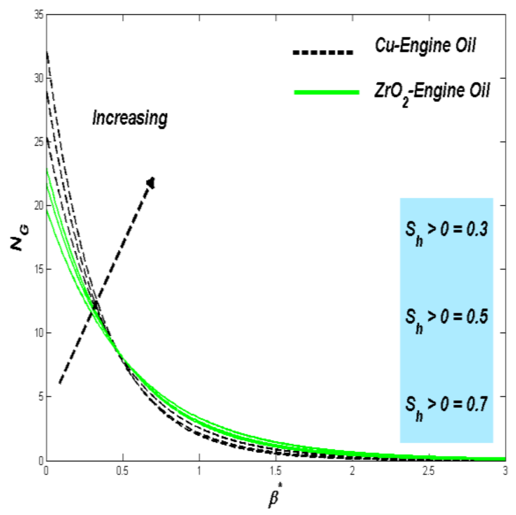
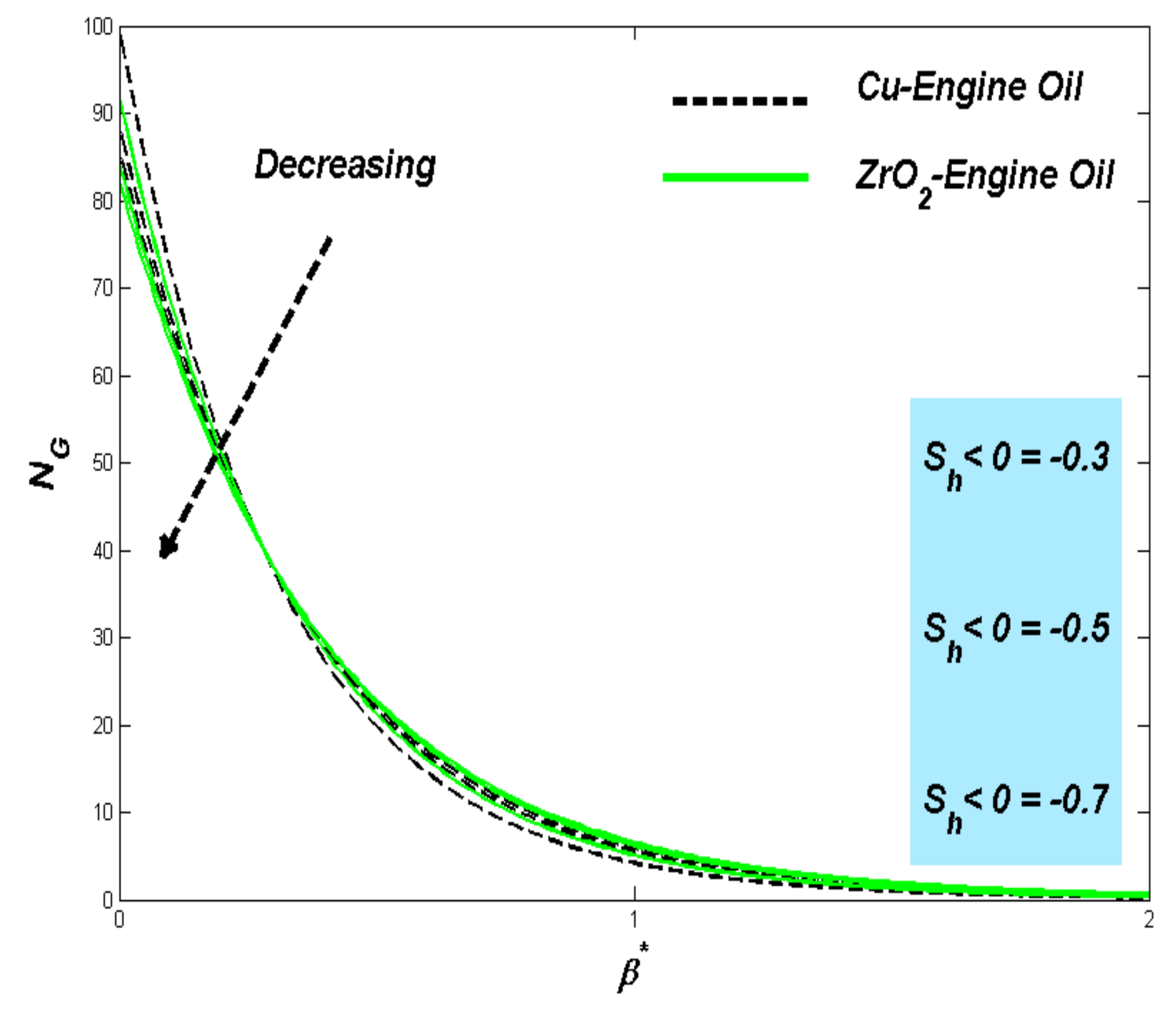
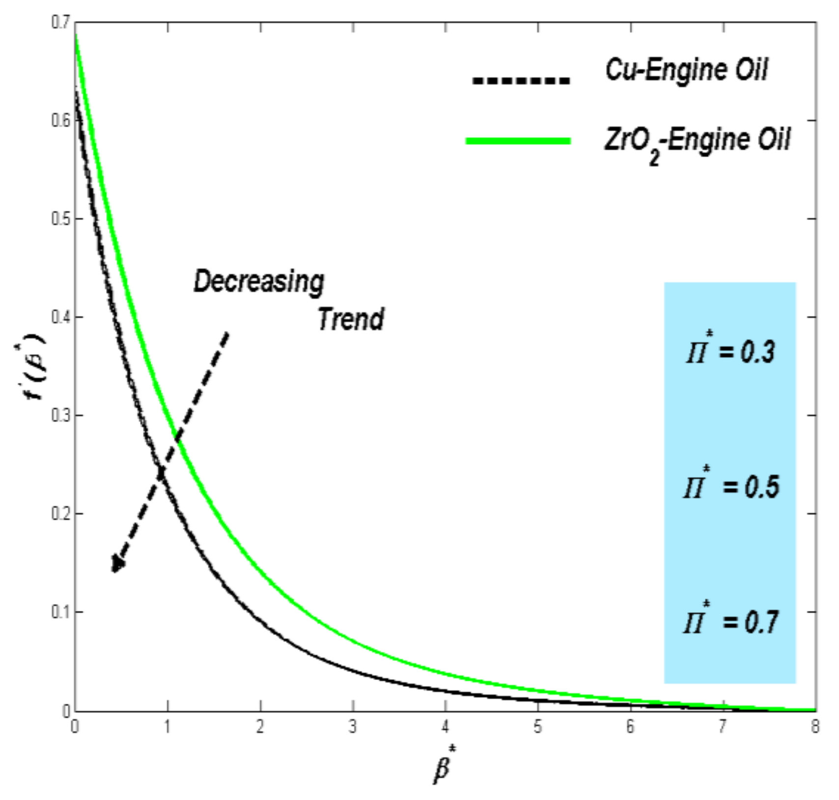
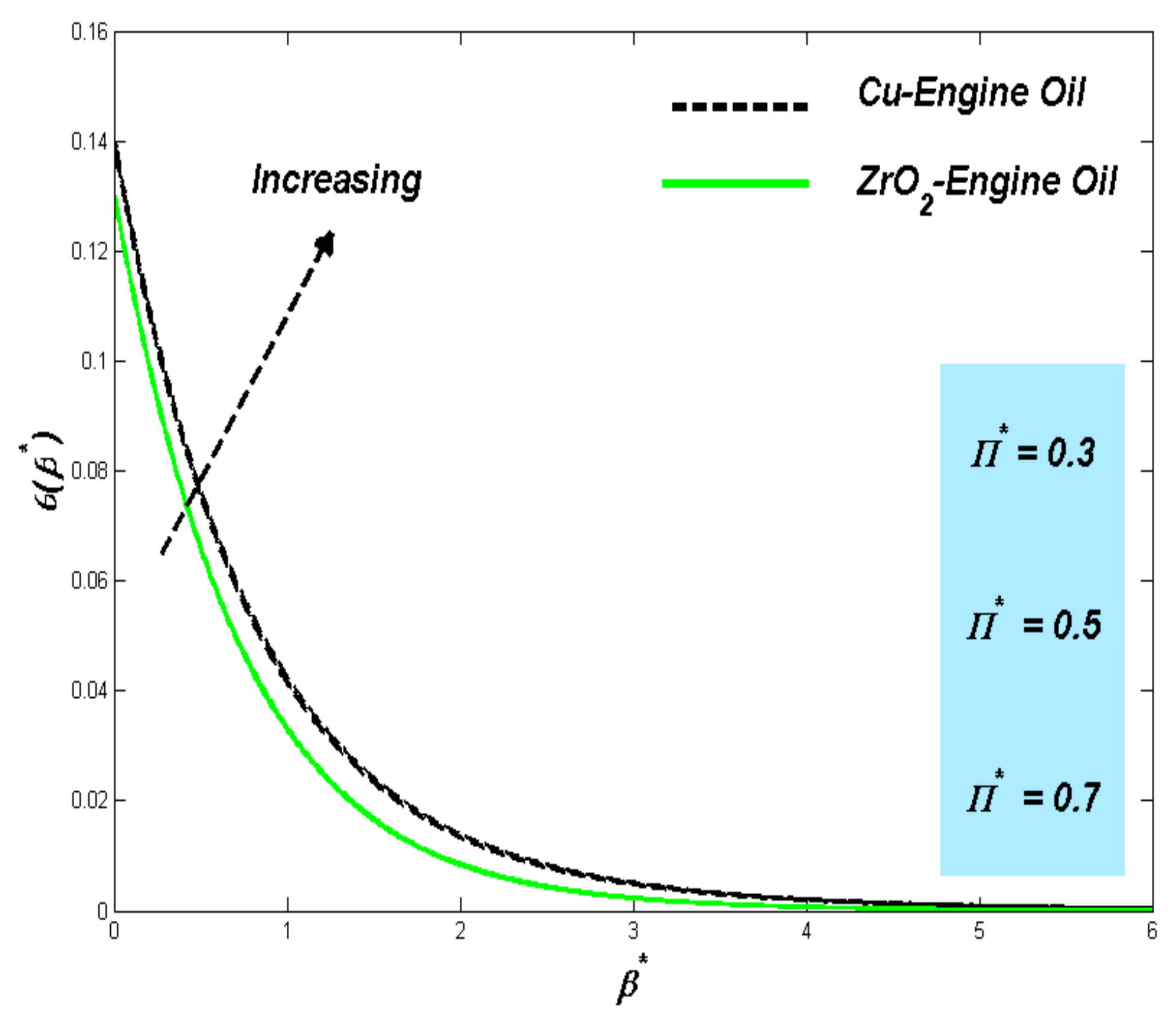
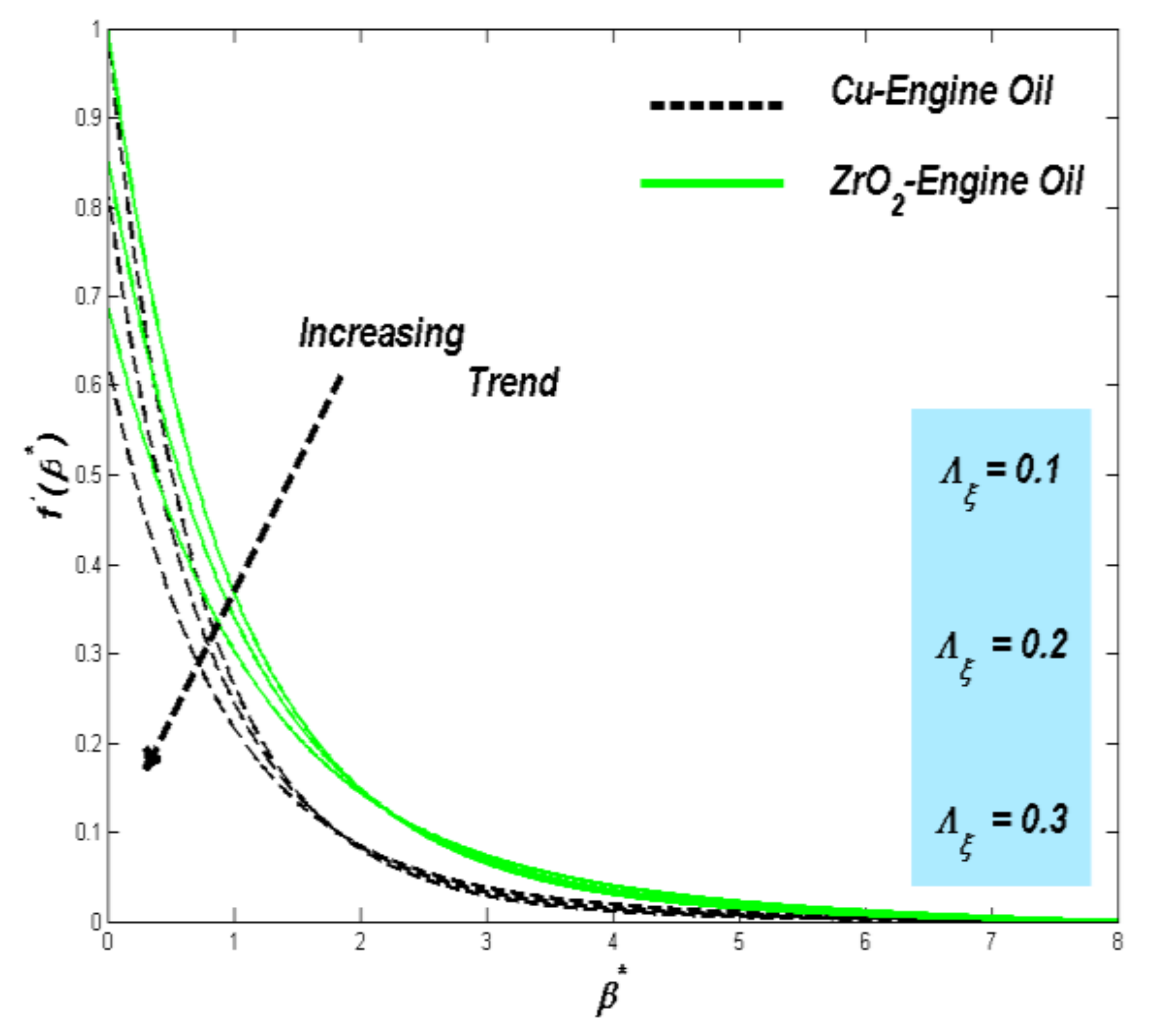
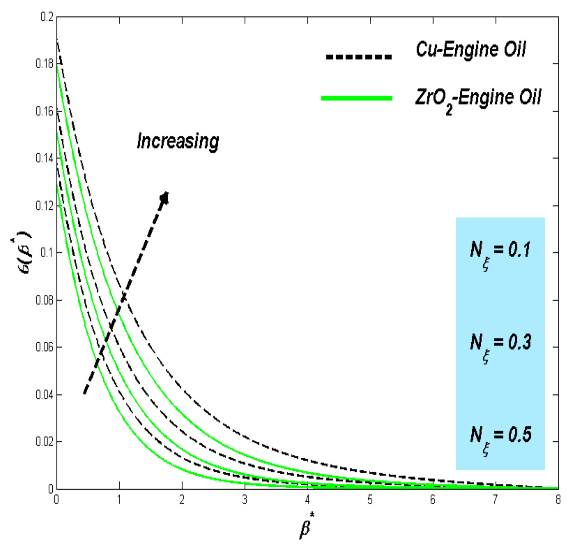
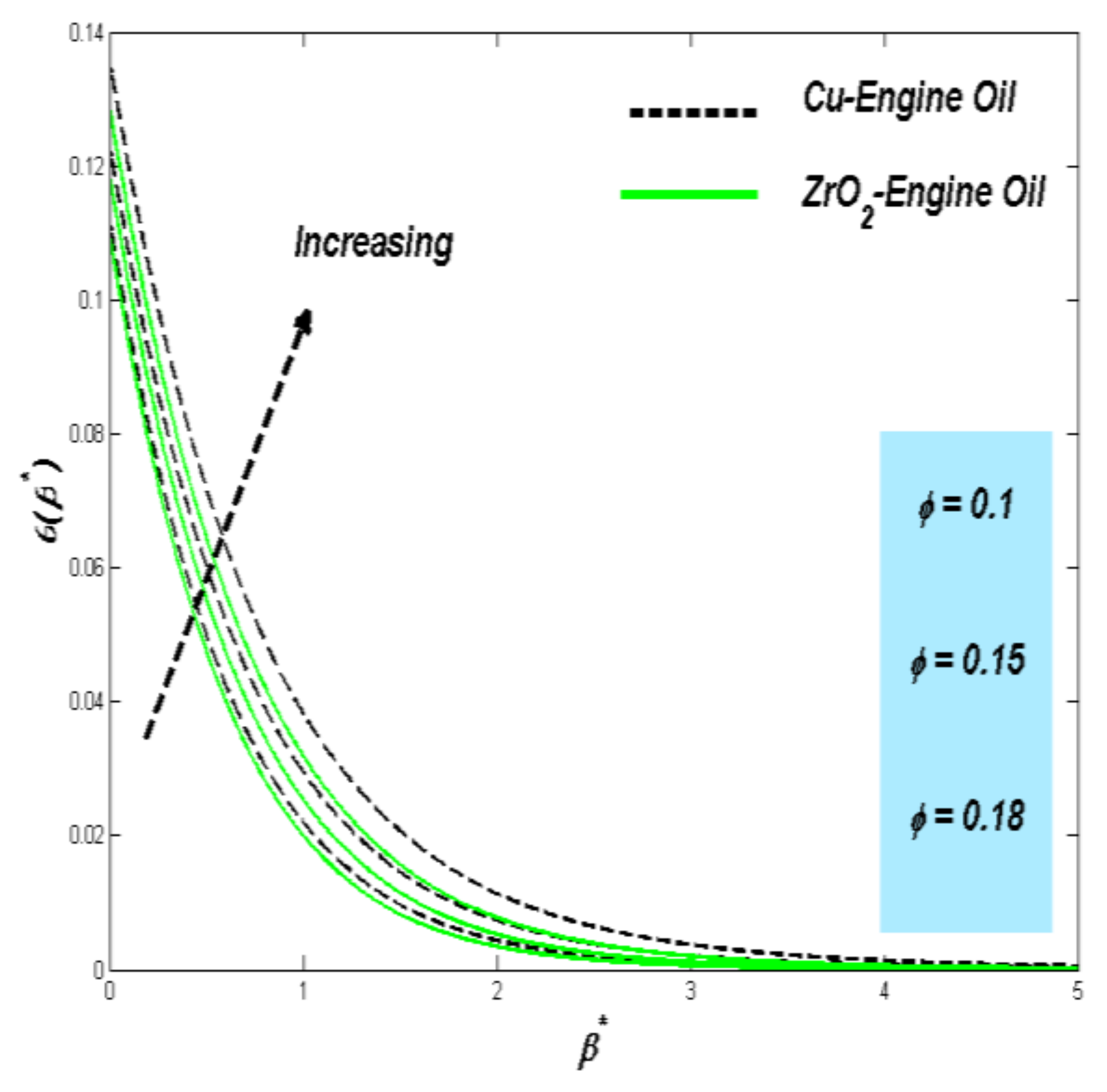
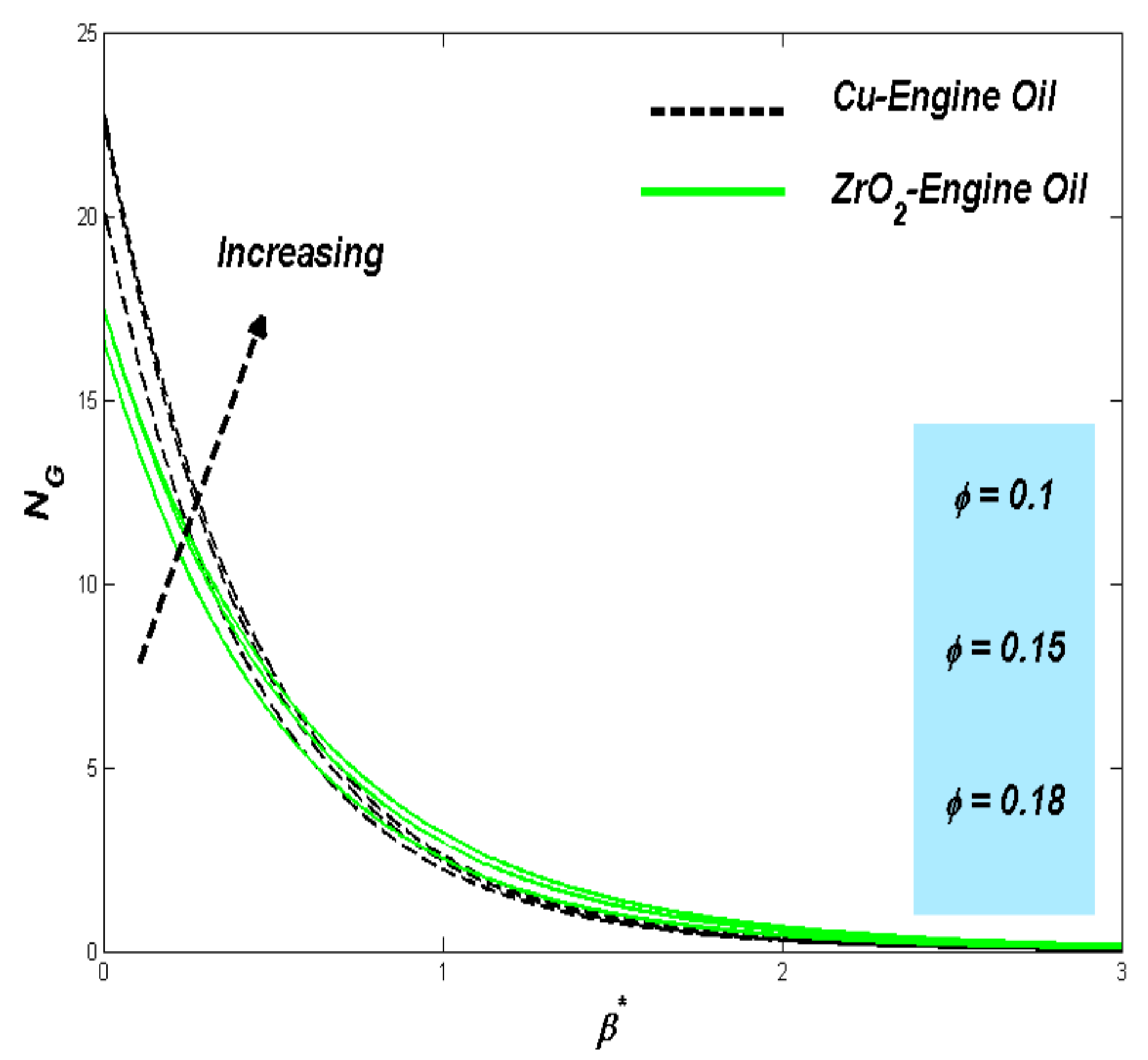
• Critical parameters such as the material parameter, the speed glide, the concentration of nanoparticles, and the injection parameter have been shown to improve the thermal boundary layer and lower the heat transfer rate of the surface. In addition, the strength of these factors enhances the flow of fluid within the boundary layer and raises the system entropy overall.
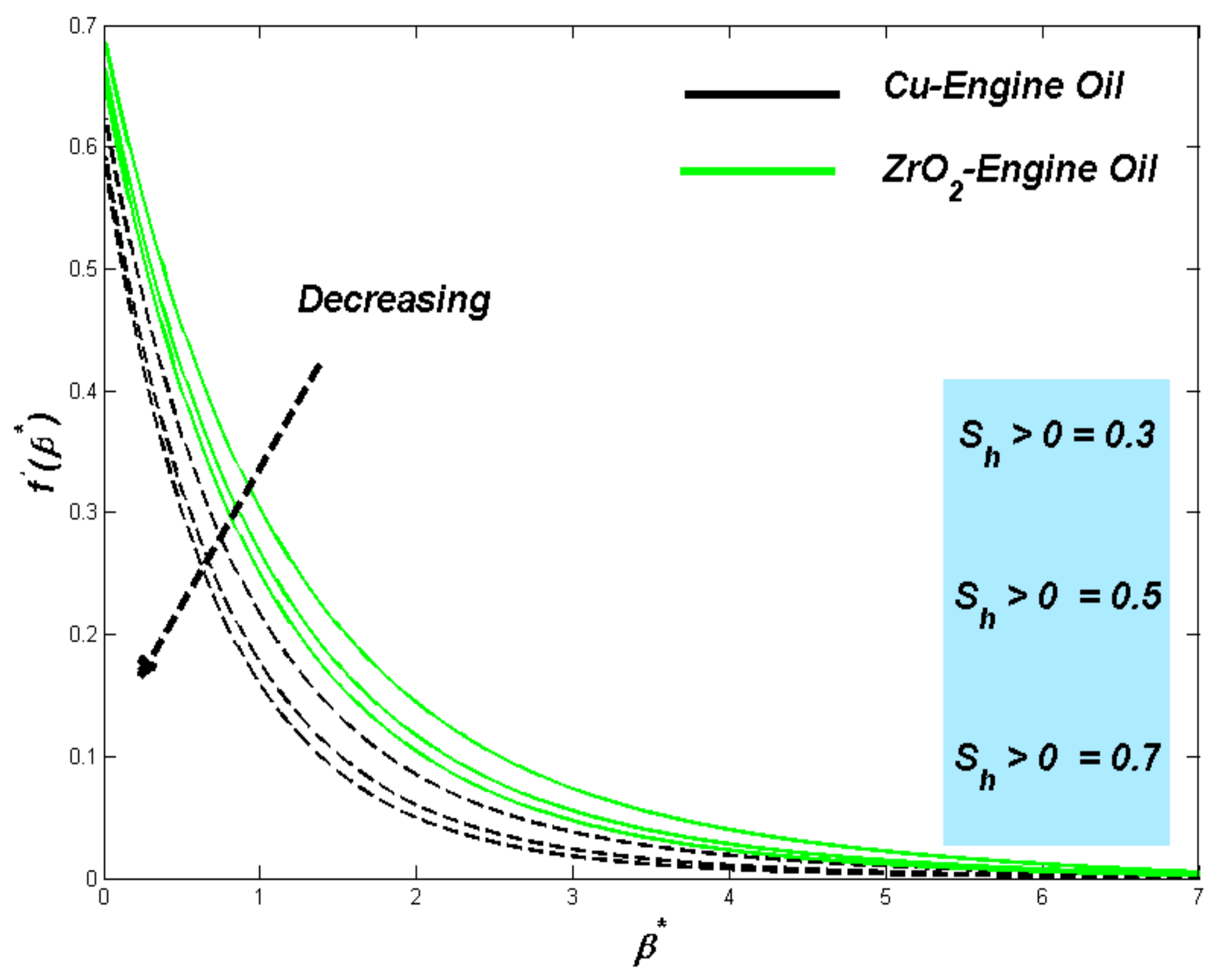
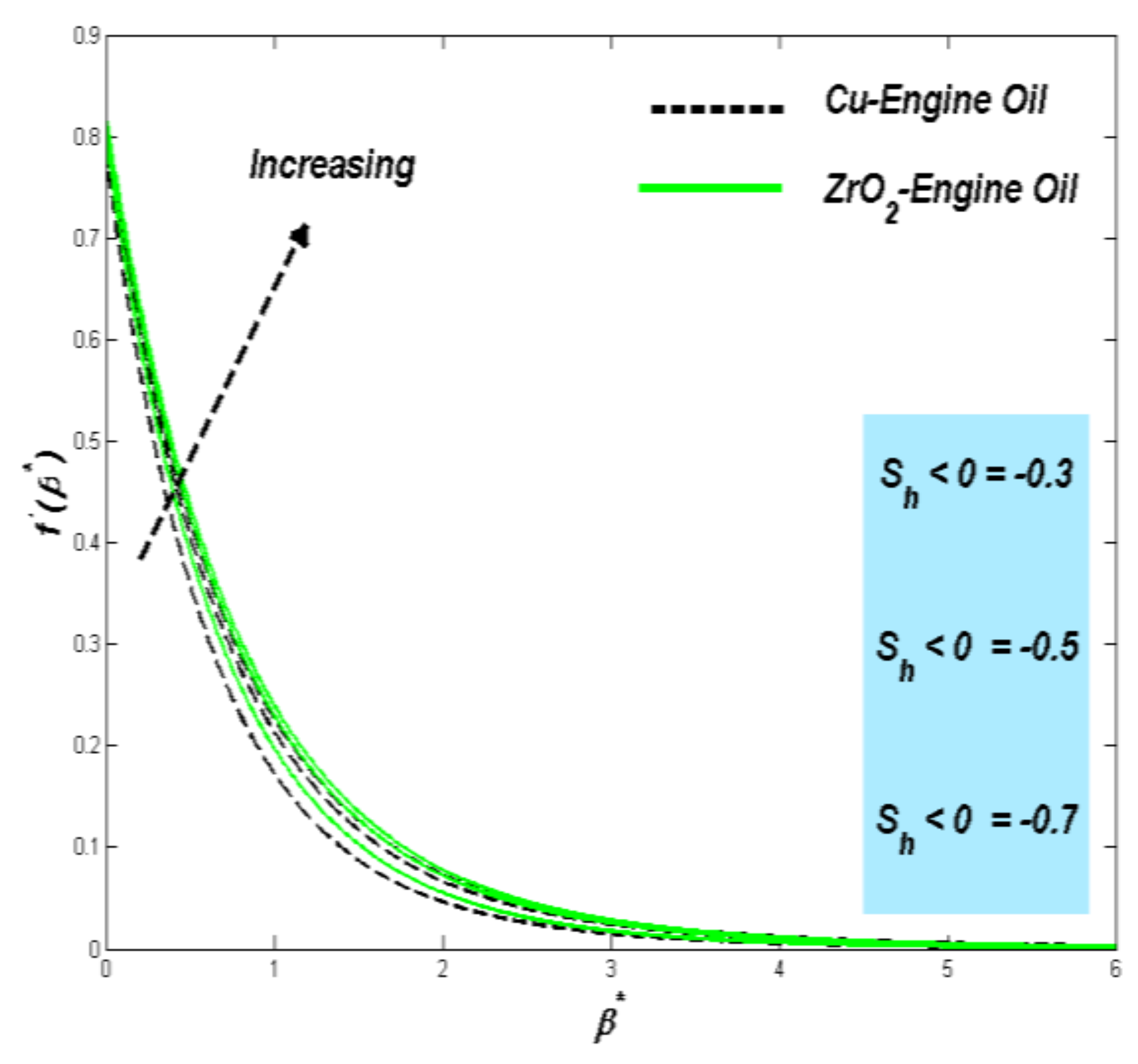
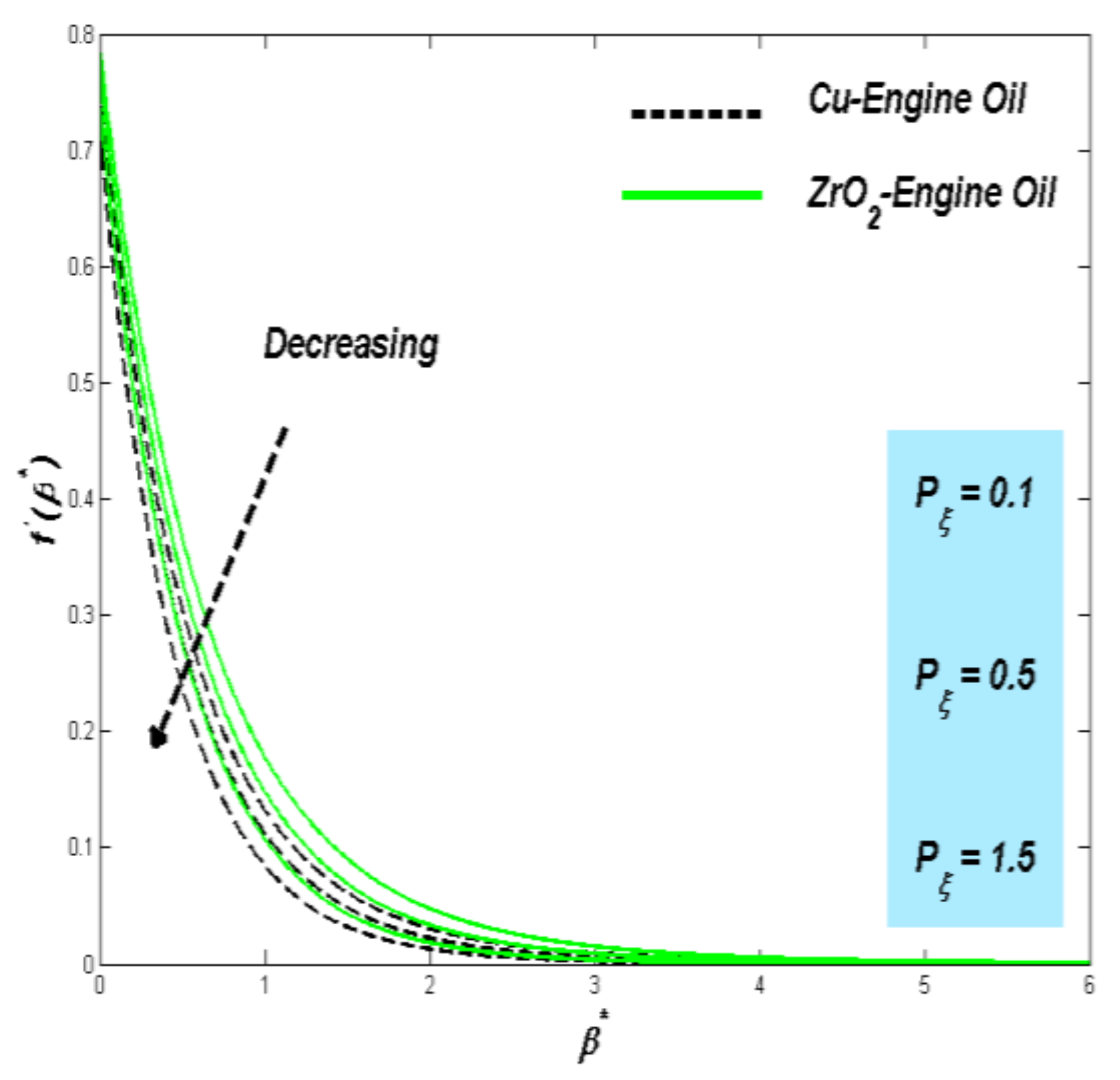
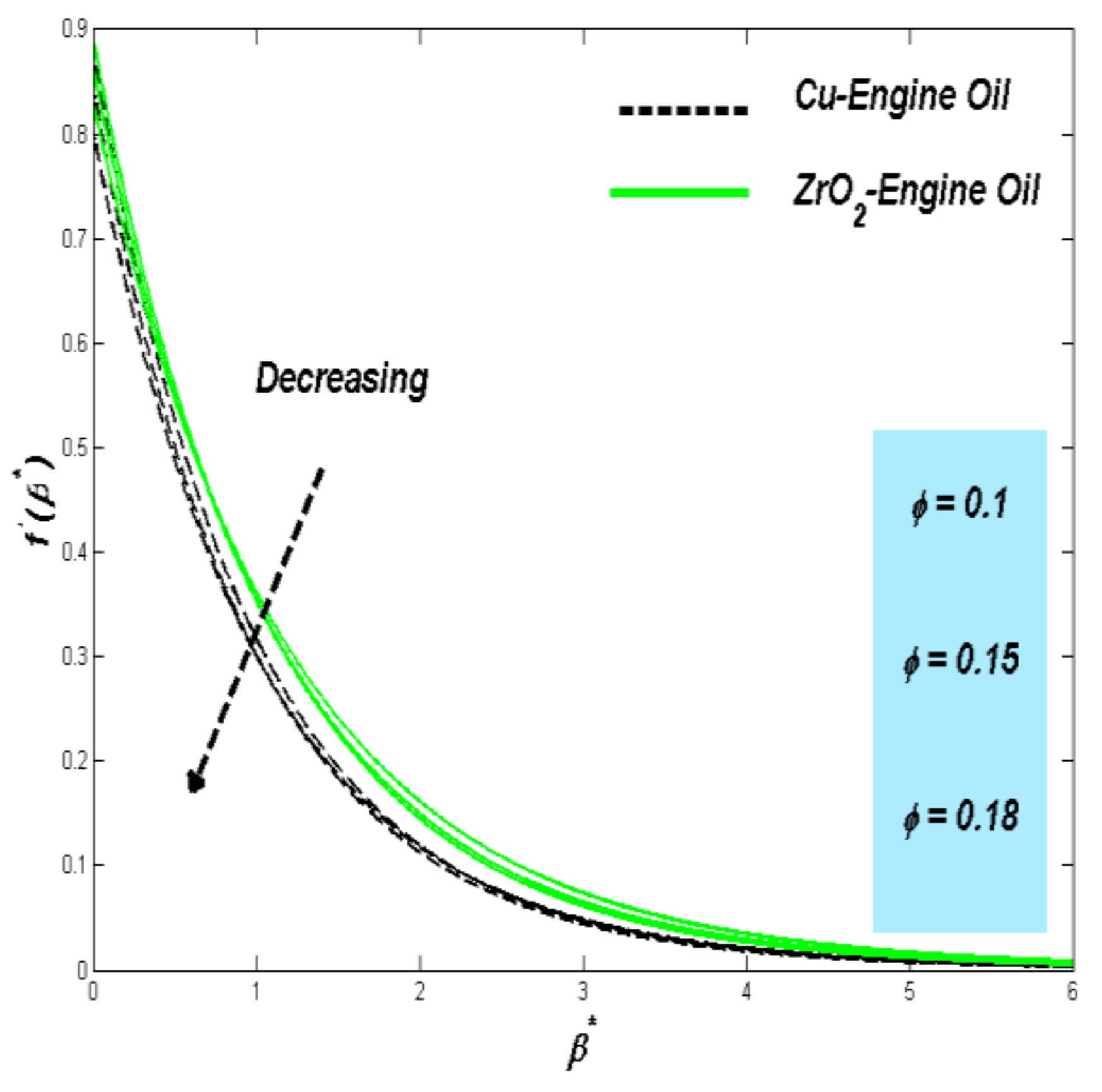
• The critical characteristics of BL collectively promote temperature variation, including slip speed, diverse thermal conductivity, non-Newtonian first-grade viscoelastic nanofluid, the concentration of nanoparticles and thermal radiation, and a high porous media. The results indicate a decreased heat transmission and a more elevated surface thermal BL. In addition, the movement diminishes as the force of the parameters specified in BL increases.
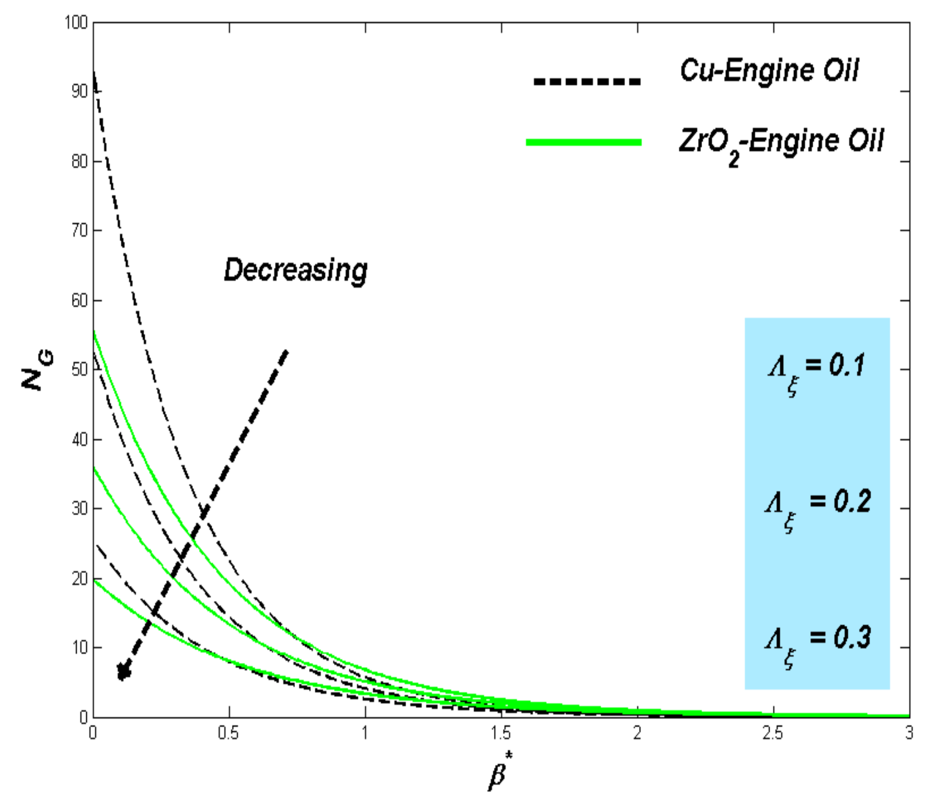
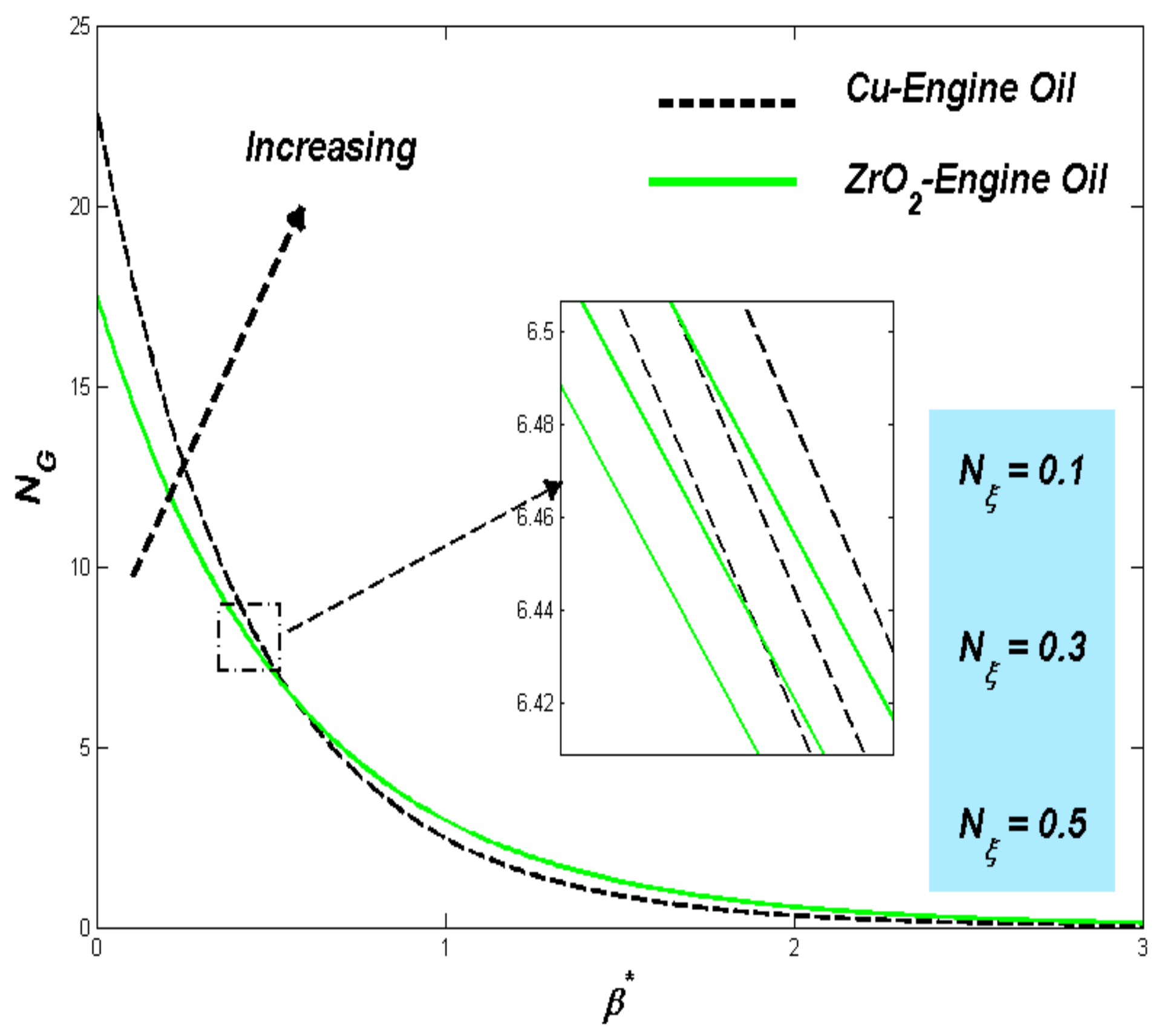
• The system’s entropy also affects the values of the number of Reynolds, the number of Brinkmann, the parameter of instability, the material parameter, the volume fraction parameter for nanoparticles, relaxation time parameter, thermal radiation, sheets convection, and the suction parameter.
• In comparison with ZrO₂-EO nanofluid, Cu-EO nanofluid is finally discovered as having a higher thermal conductivity.

The outcomes of this research can be productive as a recommended approach for future investigations in which PTSC’s thermal performance for diverse non-Newtonian nanofluids is worthy (i.e., Micropolar nanofluids, Williamson, Cross–Power law, Bird–Carreau, Second grade, and Carreau, etc.). The goals of thermal viscosity, thermally related porosity, and eminent movement of Magnetohydrodynamic can be simplified.

References

1. Safaei, M.R.; Ahmadi, G.; Goodarzi, M.S.; Kamyar, A.; Kazi, S. Boundary layer flow and heat transfer of FMWCNT/water nanofluids over a flat plate. Fluids 2016, 1, 31. [Google Scholar] [CrossRef] [Green Version]
2. Ebrahimi, D.; Yousefzadeh, S.; Akbari, O.A.; Montazerifar, F.; Rozati, S.A.; Nakhjavani, S.; Safaei, M.R. Mixed convection heat transfer of a nanofluid in a closed elbow-shaped cavity (CESC). J. Therm. Anal. Calorim. 2021, 144, 2295–2316. [Google Scholar] [CrossRef]
3. Abdollahi-Moghaddam, M.; Rejvani, M.; Alamdari, P. Determining optimal formulations and operating conditions for Al2O3/water nanofluid flowing through a microchannel heat sink for cooling system purposes using statistical and optimization tools. Therm. Sci. Eng. Prog. 2018, 8, 517–524. [Google Scholar] [CrossRef]
4. Tian, Z.; Arasteh, H.; Parsian, A.; Karimipour, A.; Safaei, M.R.; Nguyen, T.K. Estimate the shear rate & apparent viscosity of multi-phased non-Newtonian hybrid nanofluids via new developed Support Vector Machine method coupled with sensitivity analysis. Phys. A: Stat. Mech. Appl. 2019, 535, 122456. [Google Scholar]
5. Motahari, K.; Abdollahi Moghaddam, M.; Moradian, M. Experimental investigation and development of new correlation for influences of temperature and concentration on dynamic viscosity of MWCNT-SiO2 (20-80)/20W50 hybrid nano-lubricant. Chin. J. Chem. Eng. 2018, 26, 152–158. [Google Scholar] [CrossRef]
6. Nadeem, S.; Haq, R.U.; Akbar, N.S.; Khan, Z.H. MHD three-dimensional Casson fluid flow past a porous linearly stretching sheet. Alex. Eng. J. 2013, 52, 577–582. [Google Scholar] [CrossRef]
7. Jouyandeh, M.; Moayed Mohseni, M.; Rashidi, F. Forced convection heat transfer of Giesekus viscoelastic fluid in concentric annulus with both cylinders rotation. J. Pet. Sci. Technol. 2014, 4, 1–9. [Google Scholar]
8. Mohamadali, M.; Ashrafi, N. Similarity Solution for High Weissenberg Number Flow of Upper-Convected Maxwell Fluid on a Linearly Stretching Sheet. J. Eng. 2016, 2016. [Google Scholar] [CrossRef] [Green Version]
9. Jamshed, W.; Nisar, K.S.; Ibrahim, R.W.; Shahzad, F.; Eid, M.R. Thermal expansion optimization in solar aircraft using tangent hyperbolic hybrid nanofluid: A solar thermal application. J. Mater. Res. Technol. 2021, 14, 985–1006. [Google Scholar] [CrossRef]
10. Imran, M.; Farooq, U.; Waqas, H.; Anqi, A.E.; Safaei, M.R. Numerical performance of thermal conductivity in Bioconvection flow of cross nanofluid containing swimming microorganisms over a cylinder with melting phenomenon. Case Stud. Therm. Eng. 2021, 26, 101181. [Google Scholar] [CrossRef]
11. Waqas, H.; Farooq, U.; Khan, S.A.; Alshehri, H.M.; Goodarzi, M. Numerical analysis of dual variable of conductivity in bioconvection flow of Carreau–Yasuda nanofluid containing gyrotactic motile microorganisms over a porous medium. J. Therm. Anal. Calorim. 2021, 145, 2033–2044. [Google Scholar] [CrossRef]
12. Crane, L.J. Flow past a stretching plate. Z. für Angew. Math. und Phys. ZAMP 1970, 21, 645–647. [Google Scholar] [CrossRef]
13. Maleki, H.; Alsarraf, J.; Moghanizadeh, A.; Hajabdollahi, H.; Safaei, M.R. Heat transfer and nanofluid flow over a porous plate with radiation and slip boundary conditions. J. Cent. South Univ. 2019, 26, 1099–1115. [Google Scholar] [CrossRef]
14. Maleki, H.; Safaei, M.R.; Togun, H.; Dahari, M. Heat transfer and fluid flow of pseudo-plastic nanofluid over a moving permeable plate with viscous dissipation and heat absorption/generation. J. Therm. Anal. Calorim. 2019, 135, 1643–1654. [Google Scholar] [CrossRef]
15. Yarmand, H.; Ahmadi, G.; Gharehkhani, S.; Kazi, S.N.; Safaei, M.R.; Alehashem, M.S.; Mahat, A.B. Entropy generation during turbulent flow of zirconia-water and other nanofluids in a square cross section tube with a constant heat flux. Entropy 2014, 16, 6116–6132. [Google Scholar] [CrossRef] [Green Version]
16. Khosravi, R.; Rabiei, S.; Khaki, M.; Safaei, M.R.; Goodarzi, M. Entropy generation of graphene–platinum hybrid nanofluid flow through a wavy cylindrical microchannel solar receiver by using neural networks. J. Therm. Anal. Calorim. 2021, 145, 1949–1967. [Google Scholar] [CrossRef]
17. Dalir, N.; Dehsara, M.; Nourazar, S.S. Entropy analysis for magnetohydrodynamic flow and heat transfer of a Jeffrey nanofluid over a stretching sheet. Energy 2015, 79, 351–362. [Google Scholar] [CrossRef]
18. Jamshed, W.; Kumar, V.; Kumar, V. Computational examination of Casson nanofluid due to a non-linear stretching sheet subjected to particle shape factor: Tiwari and Das model. Numer. Methods Partial. Differ. Equ. 2020. [Google Scholar] [CrossRef]
19. Kotha, G.; Chamkha, A.J. Entropy generation on convectively heated surface of casson fluid with viscous dissipation. Phys. Scr. 2020, 95, 115203. [Google Scholar] [CrossRef]
20. Khan, M.; Shahid, A.; El Shafey, M.; Salahuddin, T.; Khan, F. Predicting entropy generation in flow of non-Newtonian flow due to a stretching sheet with chemically reactive species. Comput. Methods Programs Biomed. 2020, 187, 105246. [Google Scholar] [CrossRef]
21. Thumma, T.; Mishra, S.; Bég, O.A. ADM solution for Cu/CuO–water viscoplastic nanofluid transient slip flow from a porous stretching sheet with entropy generation, convective wall temperature and radiative effects. J. Appl. Comput. Mech. 2021, 1–15. [Google Scholar]
22. Usman; Ghaffari, A.; Mustafa, I.; Muhammad, T.; Altaf, Y. Analysis of entropy generation in a power-law nanofluid flow over a stretchable rotatory porous disk. Case Stud. Therm. Eng. 2021, 28, 101370. [Google Scholar] [CrossRef]
23. Aziz, A.; Shams, M. Entropy generation in MHD Maxwell nanofluid flow with variable thermal conductivity, thermal radiation, slip conditions, and heat source. AIP Adv. 2020, 10, 015038. [Google Scholar] [CrossRef] [Green Version]
24. Aziz, A.; Jamshed, W.; Aziz, T. Mathematical model for thermal and entropy analysis of thermal solar collectors by using Maxwell nanofluids with slip conditions, thermal radiation and variable thermal conductivity. Open Phys. 2018, 16, 123–136. [Google Scholar] [CrossRef]
25. Brewster, M.Q. Thermal Radiative Transfer and Properties; John Wiley & Sons: Hoboken, NJ, USA, 1992. [Google Scholar]
26. Waqas, H.; Hussain, M.; Alqarni, M.; Eid, M.R.; Muhammad, T. Numerical simulation for magnetic dipole in bioconvection flow of Jeffrey nanofluid with swimming motile microorganisms. Waves Random Complex Media 2021, 1–18. [Google Scholar] [CrossRef]
27. Jamshed, W.; Nisar, K.S.; Ibrahim, R.W.; Mukhtar, T.; Vijayakumar, V.; Ahmad, F. Computational frame work of Cattaneo-Christov heat flux effects on Engine Oil based Williamson hybrid nanofluids: A thermal case study. Case Stud. Therm. Eng. 2021, 26, 101179. [Google Scholar] [CrossRef]
28. Jamshed, W.; Aziz, A. A comparative entropy based analysis of Cu and Fe3O4/methanol Powell-Eyring nanofluid in solar thermal collectors subjected to thermal radiation, variable thermal conductivity and impact of different nanoparticles shape. Results Phys. 2018, 9, 195–205. [Google Scholar] [CrossRef]
29. Das, S.G.; Bhattacharyya, S.; Chattopadhyay, H.; Benim, A.C. Transport Phenomenon of Simultaneously Developing Flow and Heat Transfer in Twisted Sinusoidal Wavy Microchannel under Pulsating Inlet Flow Condition. Heat Transf. Eng. 2021, 1–14. [Google Scholar] [CrossRef]
30. Keller, H.B. A new difference scheme for parabolic problems. In Numerical Solution of Partial Differential Equations–II; Elsevier: Amsterdam, The Netherlands, 1971; pp. 327–350. [Google Scholar]
31. Jamshed, W.; Akgül, E.K.; Nisar, K.S. Keller box study for inclined magnetically driven Casson nanofluid over a stretching sheet: Single phase model. Phys. Scr. 2021, 96, 065201. [Google Scholar] [CrossRef]
32. Jamshed, W.; Nisar, K.S. Computational single-phase comparative study of a Williamson nanofluid in a parabolic trough solar collector via the Keller box method. Int. J. Energy Res. 2021, 45, 10696–10718. [Google Scholar] [CrossRef]
33. Kamran, A.; Hussain, S.; Sagheer, M.; Akmal, N. A numerical study of magnetohydrodynamics flow in Casson nanofluid combined with Joule heating and slip boundary conditions. Results Phys. 2017, 7, 3037–3048. [Google Scholar] [CrossRef]
34. Shahzad, F.; Jamshed, W.; Ibrahim, R.W.; Nisar, K.S.; Qureshi, M.A.; Hussain, S.M.; Isa, S.S.P.M.; Eid, M.R.; Abdel-Aty, A.-H.; Yahia, I. Comparative Numerical Study of Thermal Features Analysis between Oldroyd-B Copper and Molybdenum Disulfide Nanoparticles in Engine-Oil-Based Nanofluids Flow. Coatings 2021, 11, 1196. [Google Scholar] [CrossRef]
Figure 1. Diagram of the flow model.
Mathematics 09 02563 g001
Figure 2. Velocity profile change with S h > 0 .
Mathematics 09 02563 g002
Figure 3. Temperature profile change with S h > 0 .
Mathematics 09 02563 g003
Figure 4. Entropy profile change with S h > 0 .
Mathematics 09 02563 g004
Figure 5. Velocity profile change with S h < 0 .
Mathematics 09 02563 g005
Figure 6. Temperature profile change with S h < 0 .
Mathematics 09 02563 g006
Figure 7. Entropy profile change with S h < 0 .
Mathematics 09 02563 g007
Figure 8. Velocity profile change with Π * .
Mathematics 09 02563 g008
Figure 9. Temperature profile change with Π * .
Mathematics 09 02563 g009
Figure 10. Entropy profile change with Π * .
Mathematics 09 02563 g010
Figure 11. Velocity profile change with Λ ξ .
Mathematics 09 02563 g011
Figure 12. Temperature profile change with Λ ξ .
Mathematics 09 02563 g012
Figure 13. Entropy profile change with Λ ξ .
Mathematics 09 02563 g013
Figure 14. Velocity profile change with P ξ .
Mathematics 09 02563 g014
Figure 15. Temperature profile change with P ξ .
Mathematics 09 02563 g015
Figure 16. Entropy profile change with P ξ .
Mathematics 09 02563 g016
Figure 17. Temperature profile change with N ξ .
Mathematics 09 02563 g017
Figure 18. Entropy profile change with N ξ .
Mathematics 09 02563 g018
Figure 19. Velocity profile change with ϕ .
Mathematics 09 02563 g019
Figure 20. Temperature profile change with ϕ .
Mathematics 09 02563 g020
Figure 21. Entropy profile change with ϕ .
Mathematics 09 02563 g021