Multiscale Multiphysics Modeling of the Infiltration Process in the Permafrost

Abstract

In this work, we design a multiscale simulation method based on the Generalized Multiscale Finite Element Method (GMsFEM) for numerical modeling of fluid seepage under permafrost condition in heterogeneous soils. The complex multiphysical model consists of the coupled Richards equation and the Stefan problem. These problems often contain heterogeneities due to variations of soil properties. For this reason, we design coarse-grid spaces for the multiphysical problem and design special algorithms for solving the overall problem. A numerical method has been tested on two- and three-dimensional model problems. A a quasi-real geometry with a complex surface is considered for the three-dimensional case. We demonstrate the efficiency and accuracy of the proposed method using several representative numerical results.

1. Introduction

It is very important to consider the permafrost strata in soils under difficult climatic conditions in the Far North and the Arctic. Moreover, the structure is not constant, as many may believe, but is subject to changes as a result of thawing and freezing processes. Critical changes in structure, as a result, can lead to catastrophic consequences. Furthermore, the case with the fuel storage company NorNickel clearly demonstrates it. According to the official version, an accident occurred due to a strong thawing of the permafrost layer that led to the damage as the base could not withstand the weight of the structure. It caused irreparable ecological damage in the region and incurred colossal financial losses. In the permafrost zone, one of the main tasks in construction of buildings is a reasonable determination of the bearing capacity of permafrost soils. In addition, from a technological point of view, it is crucial to plan the start period of construction. Construction start date depends on the results of geocryological forecast and thermal engineering calculation taking into account many factors such as structure, composition, and soil properties, meteorological conditions, temperature of each engineering and geological element, the thermal effect of buildings and structures during operation. When carrying out the predictive calculations for construction under permafrost conditions, one of the important tasks is to determine the three-dimensional thermal state of soils during the operation of the structure, since the stability and reliability of the structure depend on the depth of thawing and soil temperatures. The climate is also one of the main factors in the dynamics of physical processes.

The model equations can be generalized and include sink terms due to, for example, root uptake [1,2,3]. In this case, one needs new multiscale basis functions that describe root uptake and this has not been studied in the literature. Our goal in this paper is to focus on construction related issues; however, the additional effects due to water uptake in some applications. In the paper, we design and implement Generalized Multiscale Finite Element Method (GMsFEM) for flows into heterogeneous permafrost soils. We construct a mathematical model by combining several models [4,5,6]. The seepage process is implemented using the Richards Equation [7,8,9,10,11,12,13,14,15], where the coefficients of permeability and the derivative of saturation concerning pressure are empirical dependences based on estimates of the percolation rate. The process of heat transfer in the soil is described by the heat conduction equation and takes into account the phase transition of pore moisture into ice and vice versa [16,17]. An additional convective term introduced considers the effect of saturation on temperature, and the effect of temperature on the seepage process is taken into account through the permeability coefficient [5].

Due to the multiscale nature of the problem, direct numerical simulations can be resource-intensive. For this reason, we introduce some types of upscaling or multiscale methods. These methods solve the problem on a coarse grid by introducing effective media properties or multiscale basis functions (e.g., [18,19]). The extensions of these methods to complex multiphysical problems require some special treatments. In this paper, we design GMsFEM methods for our coupled multiphysical problems. The computational algorithm is based on the GMsFEM [18,19,20,21,22,23].

We would like to highlight our contributions. In [24,25], we have considered a linear heat transfer, where the permeability does not depend on the pressure. This simplifies the algorithm as one does not need to iterate and update multiscale basis functions. In this paper, we consider the nonlinear soil model, which is more realistic. In this case, the permeability depends on the pressure and the overall multiscale procedure requires a somewhat different approach. We design multiscale basis functions and iterative methods for solving the global multiphysical problem.

Multiscale methods have become very popular in recent years and a variety of methods was developed, for example, Multiscale Finite Volume Method, Heterogeneous Multiscale Method, Multiscale Finite Element Method, Variational Multiscale Method, and so on [26,27,28,29]. For high contrast porous media, more than one degree of freedom should be introduced for accurate approximation of the processes. The main idea of GMsFEM is to apply multiscale basis functions to obtain important information in each coarse grid (computational grid) and build a reduced-order model. In this method, we construct a coarse mesh then compute the snapshot space at each coarse element and construct multiscale basis functions by performing the appropriate local spectral decomposition in each coarse block. The types of local spectral problems are motivated by analysis.

In the paper, we present several two-dimensional and three-dimensional numerical tests. In our tests, we choose parameters and test simulations by using different number of basis functions per each coarse-grid block. Our results show that using fewer basis functions, one can achieve a reasonably accurate approximation of the solution.

The work consists of 5 chapters and an introduction. The second chapter contains the statement of the problem. It discusses the process of water seepage into frozen ground. The third chapter provides a finite element approximation of the calculated mathematical model. In the fourth chapter, we demonstrate GMsFEM. The last two chapters provide numerical results for a 2D and 3D problem. The paper ends with the conclusions based on the results of calculations.

2. Mathematical Model

We consider the process of water infiltration into the ground under permafrost conditions. To do this we write down the associated mathematical model:

Seepage process. To describe the seepage process we use the Richards equation that generalizes Darcy’s law. Note that there are three different forms of writing the Richards Equation [9,10]: in terms of pressure, in terms of saturation, and mixed form. We in turn use the Richards equation written in terms of pressure:

$$m\frac{\partial s}{\partial p}\frac{\partial p}{\partial t}-\mathrm{div}(K\left(p\right)\nabla (p+z))=0,$$

(1)

here, $p=\tilde{p}/\rho g$ is head pressure, $\tilde{p}$ is pressure, m is porosity, $s\left(p\right)$ is saturation, $K\left(p\right)$ is hydraulic conductivity.

The following dependencies are true for the coefficients:

$$s\left(p\right)=1.5-exp(-\gamma p),K\left(p\right)=K_s·s{\left(p\right)}^{\sigma },$$

(2)

where $K_s$ is fully saturated conductivity, $\gamma$, $\sigma$ are problem coefficients.

Heat transfer process. To simulate the thermal regime of soils, we consider which thermal conductivity equation is used, taking into account the phase transitions of pore moisture. In practice, phase transformations occur in a small temperature range $[T^{*}-\Delta ,T^{*}+\Delta ]$. Let us take sufficiently smooth functions ${\varphi }_{\Delta }$ and ${\delta }_{\Delta }(T-T^{*})$ depending on temperature:

$${\varphi }_{\Delta }=\frac{1}{2}\left(1+\mathrm{erf}\left(\frac{T-T^{*}}{\sqrt{2}\Delta }\right)\right),{\delta }_{\Delta }(T-T^{*})=\frac{1}{\sqrt{2\pi }\Delta }\exp \left(-\frac{{(T-T^{*})}^2}{2{\Delta }^2}\right).$$

(3)

Then, we obtain the following equation for the temperature in the region $\mathsf{\Omega }$:

$$c{\rho }_{\Delta }\left(T\right)\frac{\partial T}{\partial t}-\mathrm{div}\left({\lambda }_{\Delta }\left(T\right)\mathrm{grad}T\right)=f,$$

(4)

here $c{\rho }_{\Delta }\left(T\right)=\widehat{c\rho }\left({\varphi }_{\Delta }\right)+{\rho }^{+}L{\delta }_{\Delta }(T-T^{*}),{\lambda }_{\Delta }\left(T\right)=\lambda \left({\varphi }_{\Delta }\right)$ and L is specific heat of phase transition (the latent heat). The resulting Equation (4) is a standard quasilinear parabolic equation.

For the coefficients of the equation, the following relations are true

$$\widehat{c\rho }\left({\varphi }_{\Delta }\right)={\rho }^{-}{c}^{-}+{\varphi }_{\Delta }({\rho }^{+}{c}^{+}-{\rho }^{-}{c}^{-}),\lambda \left({\varphi }_{\Delta }\right)={\lambda }^{-}+{\varphi }_{\Delta }({\lambda }^{+}-{\lambda }^{-}).$$

(5)

here, ${\rho }^{+}$, $c^{+}$, ${\lambda }^{+}$, ${\rho }^{-}$, $c^{-}$, ${\lambda }^{-}$ are density, specific heat, thermal conductivity of thawed and frozen zones, respectively.

Fully coupled. We adapt the complete physical model by analogy with [5]. The effect of saturation on temperature is taken into account by introducing an additional convective term:

$$c^{+}{\rho }^{+}(K(p,T)\nabla p,\nabla T).$$

(6)

The effect of temperature on the seepage process is taken into account through the permeability coefficient (if we mark the hydraulic permeability through $K\left(p\right)$):

$$K(p,T)=\epsilon ·K\left(p\right)+{\varphi }_{\Delta }(K\left(p\right)-\epsilon ·K\left(p\right)),$$

(7)

here, $\epsilon ={10}^{-6}$ is small number. Thus, based on (1), (2), (4), (6), (7), we write down the complete system of equations describing the seepage process in a porous medium, taking into account temperature and phase transitions.

$$\begin{array}{cc}\hfill & m\frac{\partial s}{\partial p}\frac{\partial p}{\partial t}-\mathrm{div}(K(p,T)\nabla (p+z))=0,\hfill \\ \hfill & c{\rho }_{\Delta }\left(T\right)\frac{\partial T}{\partial t}-\mathrm{div}({\lambda }_{\Delta }\left(T\right)\nabla T)+c^{+}{\rho }^{+}(K(p,T)\nabla p,\nabla T)=0.\hfill \end{array}$$

(8)

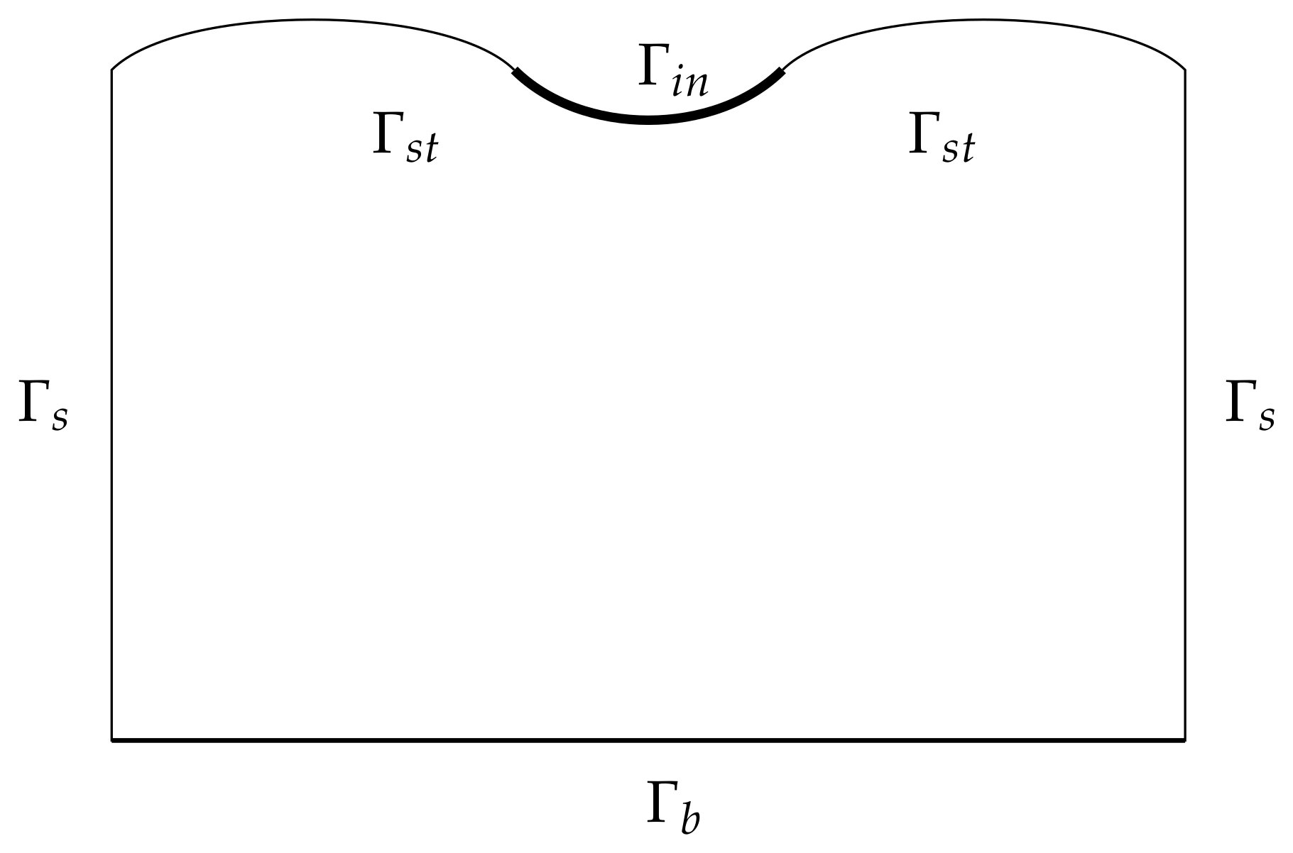
Boundary and initial conditions. We consider a quasi-real domain $\mathsf{\Omega }\subset {\mathit{R}}^2$, with boundary $\mathsf{\Gamma }=\partial \mathsf{\Omega }$, $\mathsf{\Gamma }={\mathsf{\Gamma }}_{in}+{\mathsf{\Gamma }}_{st}+{\mathsf{\Gamma }}_s+{\mathsf{\Gamma }}_b$ (see Figure 1). Let us supplement the complete system with boundary and initial conditions:

For temperature. On top of the area (${\mathsf{\Gamma }}_{st}\cup {\mathsf{\Gamma }}_{in}$):

$$-{\lambda }_{\Delta }\left(T\right)\frac{\partial T}{\partial \mathit{n}}=\beta (T-T_{air}),\mathit{x}\in {\mathsf{\Gamma }}_{st}\cup {\mathsf{\Gamma }}_{in},$$

(9)

here, $T_{air}$ is air temperature.

On the lateral and lower parts of the border:

$$-{\lambda }_{\Delta }\left(T\right)\frac{\partial T}{\partial \mathit{n}}=0,\mathit{x}\in {\mathsf{\Gamma }}_{in}\cup {\mathsf{\Gamma }}_b.$$

(10)

For pressure (saturation) there are non-flow conditions everywhere:

$$-K(p,T)(\nabla (p+z),\mathit{n})=0,\mathit{x}\in \partial \mathsf{\Omega },$$

(11)

except part ${\mathsf{\Gamma }}_{in}$, where under the condition temperature of the air is greater than fifteen degrees of Celsius:

$$p=1,\mathit{x}\in {\mathsf{\Gamma }}_{in},T_{air}>{15}^{\circ }C.$$

(12)

Initial conditions for temperature:

$$T=0,\mathit{x}\in \mathsf{\Omega },t=0.$$

(13)

Initial conditions for pressure (saturation):

$$p_1=0,p_2=0,\mathit{x}\in \mathsf{\Omega },t=0.$$

(14)

3. Fine Grid Finite Element Approximation and Picard Iteration for Linearization

To describe the approximation in time we introduce a uniform grid with a step $\tau$:

$${\overline{\omega }}_{\tau }=t^n=n\tau ,n=0,1,...,N,\tau N=T$$

(15)

and introduce the notation $p^n=p\left(t^n\right),T^n=T\left(t^n\right)$.

For approximation in time, we will use an analog of the implicit difference scheme. For the Richards equation, we use the Picard iterations, and for the Stefan equation, linearization from the previous time layer is used.

$$\begin{array}{cc}\hfill & m\frac{\partial s}{\partial p}\left(p^k\right)\frac{p^{k+1}-p^n}{\tau }-\mathrm{div}(K(p^k,T^n)\nabla (p^{k+1}+z))=0,k=0,1,...\hfill \\ \hfill & c{\rho }_{\Delta }\left(T^n\right)\frac{T^{n+1}-T^n}{\tau }-\mathrm{div}({\lambda }_{\Delta }\left(T^n\right)\nabla T^{n+1})+c^{+}{\rho }^{+}(K(p^{n+1},T^n)\nabla p^{n+1},\nabla T^n)=0,\hfill \end{array}$$

(16)

where k are Picard iterations. Only after solving the equation for p can we calculate the equation for T using $p^{n+1}=p^{k+1}$.

For the approximation in space, standard Lagrangian finite elements are used. Next, we introduce the space of finite elements:

$$\begin{array}{cc}\hfill & V_T=\widehat{V_T}=H^1\left(\mathsf{\Omega }\right),\hfill \\ & V_p=\{v\in H^1\left(\mathsf{\Omega }\right):v\left(\mathit{x}\right)=1,\mathit{x}\in \mathsf{\Omega }\},\hfill \\ & \widehat{V_p}=\{v\in H^1\left(\mathsf{\Omega }\right):v\left(\mathit{x}\right)=0,\mathit{x}\in \mathsf{\Omega }\},\hfill \end{array}$$

and introduce finite-dimensional spaces $V_T^h,\widehat{V_T^h}\subset V_T,V_p^h,\widehat{V_p^h}\subset V_p$. Here $H^1\left(\mathsf{\Omega }\right)$—Sobolev space. Next, we represent the system in a variational form (16). Thus, we obtain a variational formulation with taking into account the boundary conditions:

$$\begin{array}{cc}\hfill m{\int }_{\mathsf{\Omega }}\frac{\partial s}{\partial p}\left(p^k\right)\frac{p^{k+1}-p^n}{\tau }{v}_{1}d\mathit{x}+{\int }_{\mathsf{\Omega }}(K(p^k,T^n)\nabla (p^{k+1}+z),\nabla v_1)d\mathit{x}=0& ,k=0,1,...\hfill \\ \\ \hfill {\int }_{\mathsf{\Omega }}c{\rho }_{\Delta }\left(T^n\right)\frac{T^{n+1}-T^n}{\tau }{v}_{2}d\mathit{x}+{\int }_{\mathsf{\Omega }}({\lambda }_{\Delta }\left(T^n\right)\nabla T^{n+1},\nabla v_2)d\mathit{x}+\\ \hfill +{\int }_{\mathsf{\Omega }}{c}^{+}{\rho }^{+}(K(p^{n+1},T^n)\nabla p^{n+1},\nabla T^n)v_{2}d\mathit{x}+{\int }_{{\mathsf{\Gamma }}_{st}\cup {\mathsf{\Gamma }}_{in}}\beta (T^{n+1}& -T_{air})v_{2}d\mathit{s}=0.\hfill \end{array}$$

(17)

here, $v_1\in \widehat{V_p^h}$ and $v_2\in \widehat{V_T^h}$.

4. Generalized Multiscale Finite Element Method

In this section, we describe how to build a local reduced-order model on a snapshot space by solving some local spectral problems using GMsFEM. First, we need to generate a rough mesh and build a snapshot space. Then, we solve special spectral problems in these snapshot spaces for each coarse grid block we get some kind of set of multiscale basis functions. Thus, it can be seen that the key component of the GMsFEM method is the construction of local basis functions.

In offline computation, we have to build a snapshot of the $V_{snap}^{{\omega }_i}$ space for each rough neighborhood ${\omega }_i$. The snapshot space can be the space of all small-scale basis functions or solutions of some local problems on ${\omega }_i$ with all possible boundary conditions.

$$\begin{array}{cc}\hfill -\mathrm{div}(K_S\left(x\right)\nabla {\psi }_j)=0& ,x\in {\omega }_i,\hfill \\ \hfill {\psi }_j={\delta }_j\left(x\right)& ,x\in \partial {\omega }_i,\hfill \end{array}$$

here, ${\delta }_j\left(x\right)$ some set of functions defined on $\partial {\omega }_i$, $j=1,\dots ,J_i$ ($J_i$ number of all nodes $\partial {\omega }_i$). Therefore, we define

$$V_{\mathrm{snap}}=\mathrm{span}\{{\psi }_j^{\mathrm{snap}}:1\le j\le J_i\},\mathrm{and}{R}_{\mathrm{snap}}=[{\psi }_1^{\mathrm{snap}},\dots ,{\psi }_{J_i}^{\mathrm{snap}}].$$

Offline space is constructed using the following local spectral problems in snapshot space:

$$A^{\mathrm{off}}{\mathsf{\Psi }}_k^{\mathrm{off}}={\lambda }_k^{\mathrm{off}}{S}^{\mathrm{off}}{\mathsf{\Psi }}_k^{\mathrm{off}},$$

here, $A^{\mathrm{off}}=R_{\mathrm{snap}}A{R}_{\mathrm{snap}}^T$, $S^{\mathrm{off}}=R_{\mathrm{snap}}S{R}_{\mathrm{snap}}^T$. Here $A\mathrm{and}S$ denote similar fine-scale matrices defined as follows:

$$\begin{array}{c}\hfill A=\left[a_{mn}\right]={\int }_{{\omega }_i}{K}_s\left(x\right)\nabla {\varphi }_m·\nabla {\varphi }_{n}dx,S=\left[s_{mn}\right]={\int }_{{\omega }_i}{K}_s\left(x\right){\varphi }_m{\varphi }_{n}dx,\end{array}$$

here, ${\varphi }_m$ are linear basis functions.

To generate the offline space, choose the smallest $M_{\mathrm{off}}^{{\omega }_i}$ eigenvalues and find the corresponding eigenvectors ${\psi }_k^{\mathrm{off}}={\sum }_m{\mathsf{\Psi }}_{k,m}^{\mathrm{off}}{\varphi }_m^{\mathrm{off}}$ for $k=1,\dots ,M_{\mathrm{off}}^{{\omega }_i}$.

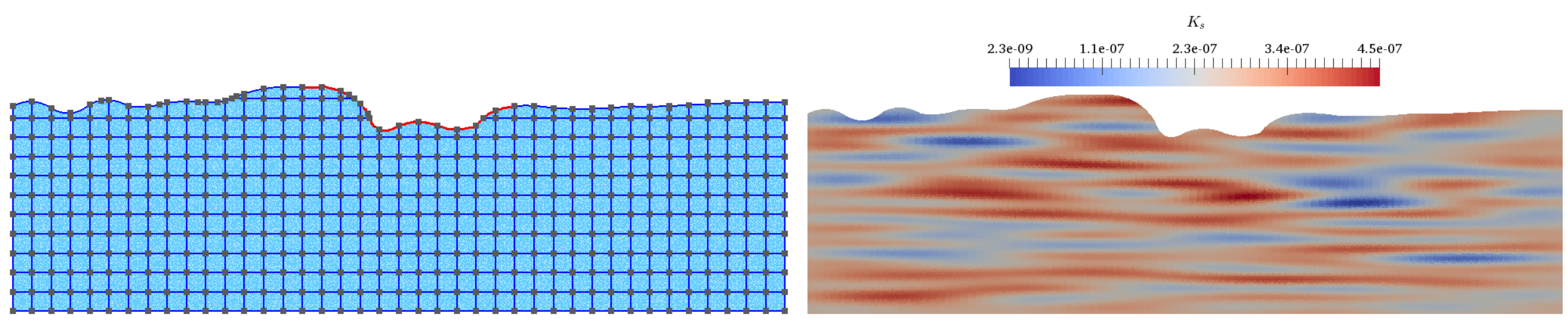
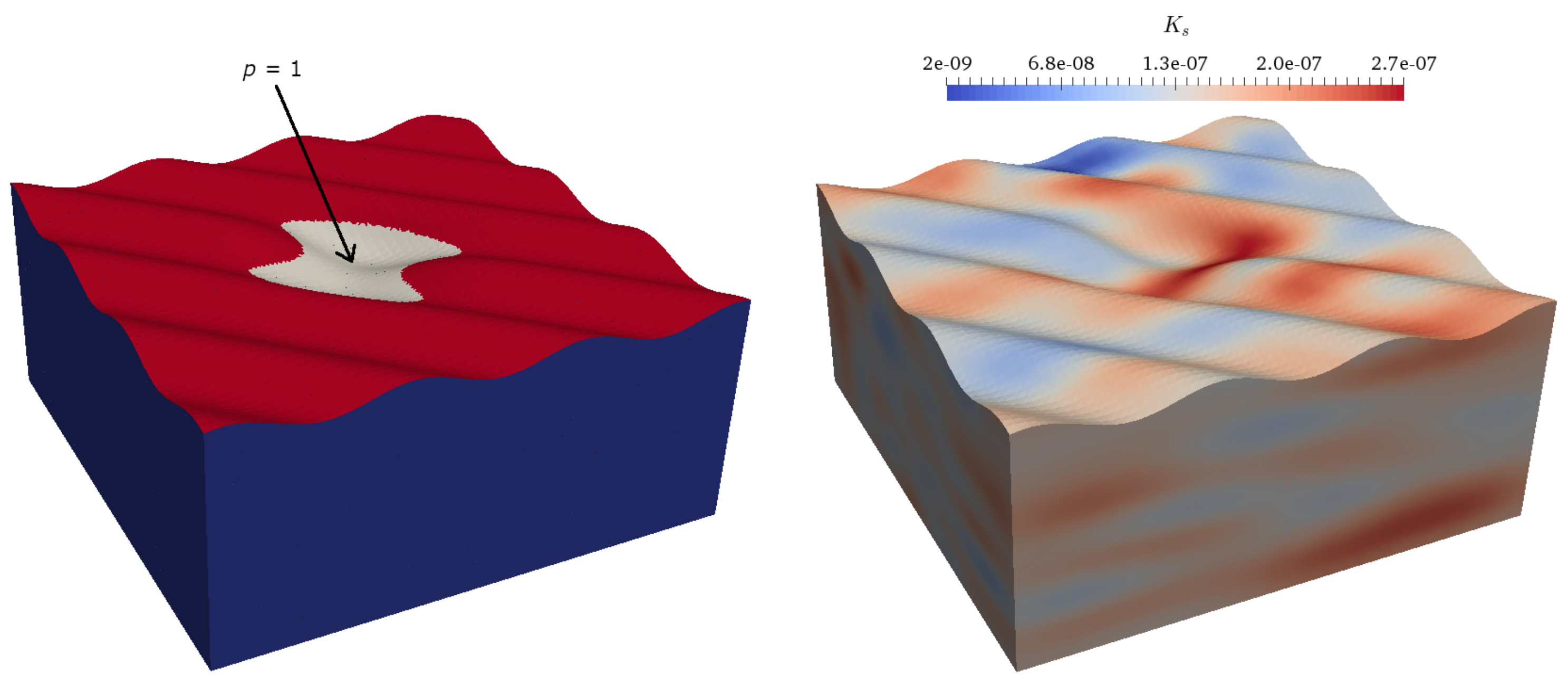
We implement special multiscale basis functions ${\varphi }_j^i$ (Figure 2) to describe near surface form effects. We must multiply the found eigenvectors by the partition of unity functions ${\chi }_i$.

$${\varphi }_k^i={\chi }_i{\psi }_k^{\mathrm{off}}\mathrm{for}1\le i\le N\mathrm{and}1\le k\le M_{\mathrm{off}}^{{\omega }_i},$$

here, $M_{\mathrm{off}}^{{\omega }_i}$ denotes the number of eigenvectors that are sampled for each local area ${\omega }_i$.

To define a partition of unity function, we first define an initial coarse space $V_0^{\mathrm{init}}=\mathrm{span}{\left\{{\chi }_i\right\}}_{i=1}^N$; here, N the number of rough neighborhoods and ${\chi }_i$ is a standard multiscale partition of unity function which is defined by:

$$\begin{array}{c}\hfill -\mathrm{div}(K_s\left(x\right)\nabla {\chi }_i)=0,C\in {\omega }_i,\\ \hfill {\chi }_i=g_i,\mathrm{on}\partial C,\end{array}$$

where $g_i$ is a continuous function on $\partial C$ and linear on each edge $\partial C$; here, C is the cell of the coarse grid.

Next, we define a multiscale space:

$$V_{\mathrm{off}}=\mathrm{span}\{{\varphi }_k^i:1\le i\le N\mathrm{and}1\le k\le M_{\mathrm{off}}^{{\omega }_i}\}$$

and define the projection matrix:

$$R={[{\varphi }_1^1,\dots ,{\varphi }_{M^1}^1,\dots ,{\varphi }_1^N,\dots ,{\varphi }_{M^N}^N]}^T.$$

In this problem, obtained basis functions are used to solve a fully coupled problem. Using the projection matrix R, we solve the problem using a coarse grid:

$$M_c\frac{u_c^n-u_c^{n-1}}{\tau }+A_c{u}_c^n=F_c,$$

(18)

where $M_c=RN{R}^T$, $A_c=RA{R}^T$, $F_c=RF$ and $u_{ms}^n=R^T{u}_c^n$; here, $u_{ms}^n$ is a fine-grid projection of the coarse-grid solution. M and A are the mass and stiffness matrices for the Fine system, respectively, F is the vector of the right-hand side and u is the required function for the pressure P and T.

5. Numerical Results Two-Dimensional Problem

Numerical simulation of an applied problem in a two-dimensional formulation describing water seepage into the permafrost. The object dimension is 10 m wide and 5 m deep (Figure 3).

In an open area boundary conditions of the third kind were used—the external environment. For the parameters of the external environment, the monthly average values of air temperature were taken in the area of Yakutsk for the last year (

Table 1. Average air temperature.

Month	Temperature ${}^{\circ }$C
January	−36.0
February	−31.9
March	−17.7
April	−2.8
May	7.7
June	16.7
July	19.8
August	17.3
September	6.6
October	−4.7
November	−25.2
December	−36.4

).

In these calculations, it was assumed that the heat flow from the bowels would not affect the temperature distribution of the rocks; therefore, the homogeneous Neumann boundary condition was taken at the lower boundary of the computational domain.

We implement numerical modeling of the problem under consideration for the following values of the thermophysical properties of the soil:

•

Problem parameters $\sigma =2.0$, $\gamma =1.0$, $\beta =14.0$;

•

Volumetric heat capacity $c\rho$—thawed zone $2397.6\times {10}^3$ [J/m${}^3·$K]; frozen zone $1886.4\times {10}^3$ [J/m${}^3·$K];

•

Thermal conductivity $\alpha$—thawed zone $1.37$ [W/m·K], frozen zone $1.72$ [W/m·K];

•

Phase transition ${\rho }^{+}L$—75,330 $\times {10}^3$ [J/m].

The soil has an initial temperature $-1.5{}^{\circ }$C, pressure is equal 0. Calculations are carried out for 365 days (1 year). For Picard iterations we use $ϵ=1\%$.

For numerical comparison of the fine–scale and multiscale solutions, we use weighted relative $L_2$ and energy errors for temperature and pressure:

$${\left|\right|e\left|\right|}_{L_2}=\sqrt{\frac{{\int }_{\mathsf{\Omega }}{(u_h-u_{ms})}^{2}dx}{{\int }_{\mathsf{\Omega }}{u}_h^{2}dx}}{,\left|\right|e\left|\right|}_a=\sqrt{\frac{a_{\varphi }(u_h-u_{ms},u_h-u_{ms})}{a_{\varphi }(u_h,u_h)}},$$

where $u_h$ and $u_{ms}$ are the fine–scale and multiscale solutions.

Table 2. Relative $L_2$ and energy errors (%) for different number of multiscale basis functions. ($DO{F}_f=$ 29,041).

M	DOF	${\left|\right|\mathit{e}\left|\right|}_{{\mathit{L}}^2}$	${\left|\right|\mathit{e}\left|\right|}_{\mathit{a}}$	M	DOF	${\left|\right|\mathit{e}\left|\right|}_{{\mathit{L}}^2}$	${\left|\right|\mathit{e}\left|\right|}_{\mathit{a}}$
$20\times 5$ coarse grid
$t=150$
	Temperature				Pressure
1	496	3.97	21.96	1	496	2.28	29.78
2	992	2.06	15.29	2	992	1.14	21.3
4	1984	0.88	9.43	4	1984	0.65	16.05
8	3968	0.33	4.97	8	3968	0.28	10.02
16	7936	0.07	1.91	16	7936	0.09	4.89
$t=200$
	Temperature				Pressure
1	496	2.77	14.78	1	496	2.19	29.06
2	992	1.3	10.9	2	992	0.82	21.3
4	1984	0.62	7.35	4	1984	0.46	16.53
8	3968	0.23	4.26	8	3968	0.16	8.56
16	7936	0.03	1.18	16	7936	0.04	3.83

shows the relative errors of $L2$ and energies for a different number of multiscale basis functions. First of all, we noticed that by updating the basis functions more often we can get more accurate solutions. We obtain $0.82\%L2$ error for the pressure and $1.3\%L2$ error for temperature on 2 multiscale basis functions. On the other hand accuracy of the method increase on 8 multiscale basis functions. In this case, method provide $0.16\%L2$ error for the pressure, and $0.23\%$ for temperature.

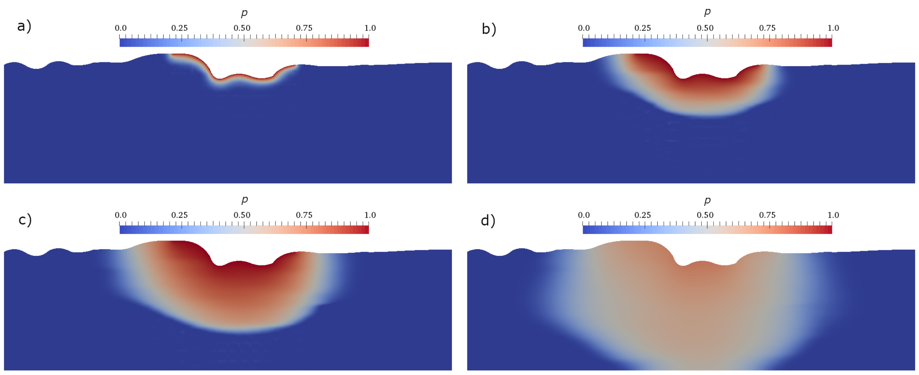
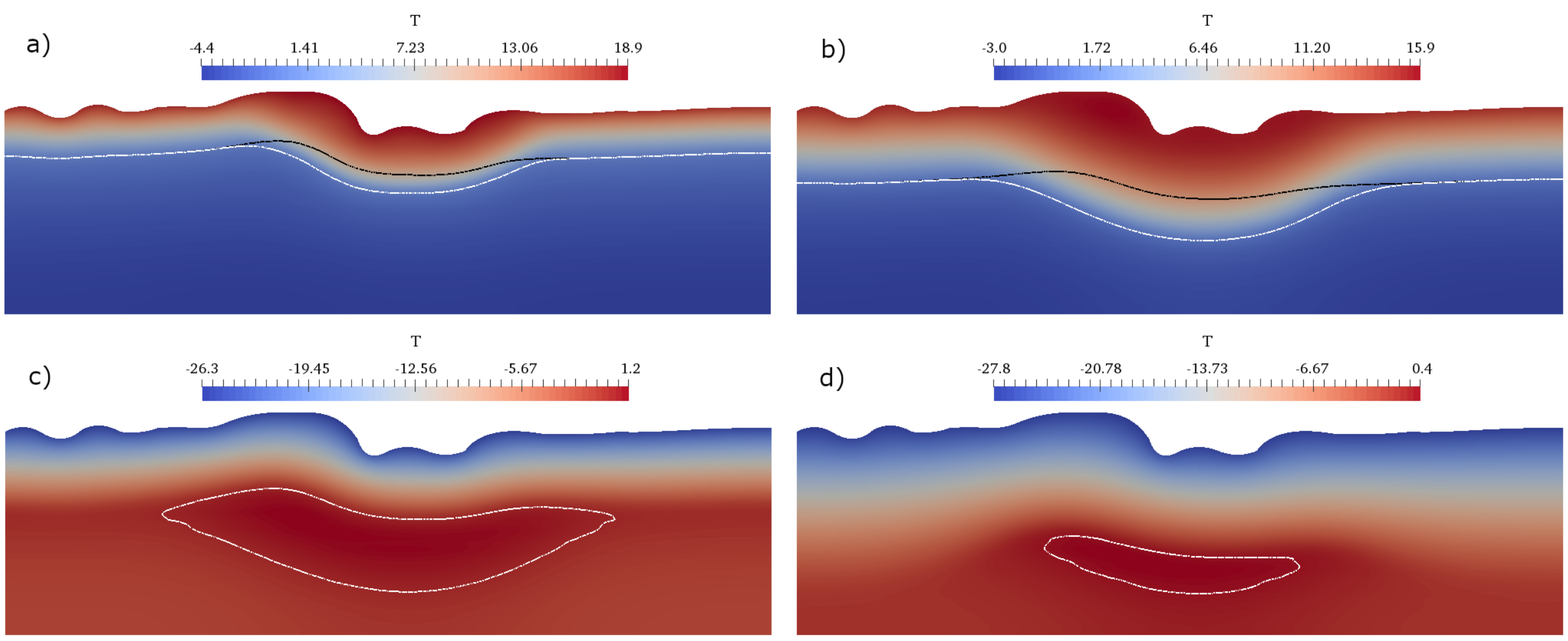
The coarse grid solution using 8 basis functions for each temperature and pressure are shown in Figure 4 and Figure 5 for four time steps.

Figure 5 demonstrates zero isoclines (phase transition). The white line indicates saturated soil and the black line unsaturated soil. The thawed layer lasts longer when a layer is saturated and this can lead to dangerous consequences.

6. Numerical Results Three-Dimensional Problem

We expand the 2D problem to the problem in a three-dimensional setting (Figure 6). The area in the plan has the same dimensions of 10 m and a height of 6 m. The computational grid has the dimensions $N_n=$ 522,774 and $N_e=$ 35,844,142. All characteristics of the problem remain the same as in the case of 2D. The calculations were carried out for 1 year with a time step of $\tau =24$ h. To generate the soil surface, we used the following surface equation $z(x,y)=5.5+0.5sin(x+y)-0.2exp(-0.5[{(5-x)}^2-{(5-y)}^2]/10)$. At the center of this geometry, there is a pronounced depression through which liquid seeps. This depression serves as an analog of places where water from precipitation accumulates.

Table 3. Relative $L_2$ and energy errors (%) for different number of multiscale basis functions. ($DO{F}_f=$ 522,774).

M	DOF	${\left|\right|\mathit{e}\left|\right|}_{{\mathit{L}}^2}$	${\left|\right|\mathit{e}\left|\right|}_{\mathit{a}}$	M	DOF	${\left|\right|\mathit{e}\left|\right|}_{{\mathit{L}}^2}$	${\left|\right|\mathit{e}\left|\right|}_{\mathit{a}}$
$20\times 20\times 8$ coarse grid
$t=150$
	Temperature				Pressure
1	3969	3.27	16.8	1	3969	9.17	36.26
2	7938	2.67	14.75	2	7938	4.34	24.83
4	15,876	0.97	8.87	4	15,876	2.31	19.6
8	31,752	0.6	6.96	8	31,752	1.22	16.17
16	63,504	0.3	4.27	16	63,504	0.67	12.92
$t=200$
	Temperature				Pressure
1	3969	2.71	13.87	1	3969	8.57	31.61
2	7938	1.5	11.1	2	7938	3.63	20.53
4	15,876	0.66	6.35	4	15,876	1.89	15.09
8	31,752	0.43	5.53	8	31,752	1.01	12.26
16	63,504	0.18	3.12	16	63,504	0.52	9.04

demonstrates numerical convergences in norm ${\left|\right|e\left|\right|}_{L^2}$ and ${\left|\right|e\left|\right|}_a$ for temperature and pressure. Methodical results for the three-dimensional case qualitatively repeat calculations in two-dimensional calculations. At the same time, the main trends persist and a decrease in the error can be observed with an increase in the number of multiscale basis functions. The main computational difficulty is localized in the Richards equation. This fact can be described by the error in ${\left|\right|e\left|\right|}_a$ norm. This is due to the non-linearity of the equation complicated by the complex permeability coefficient which depends on the temperature. This can be dealt with by an increasing number of multiscale basis embassies. On the other hand, the average ${\left|\right|e\left|\right|}_{L^2}$ error demonstrates good accuracy of the applied method. Already good accuracy is achieved when 16 multiscale basis functions are implemented. We obtain $0.52\%L2$ error for the pressure and $0.18\%L2$ error for temperature on 16 multiscale basis functions. Discussed $L2$ norms are observed to provide smaller errors because they do not contain gradients. It is known that the gradients of multiscale functions are rough, and these spatial fields are more difficult to represent with multiscale methods.

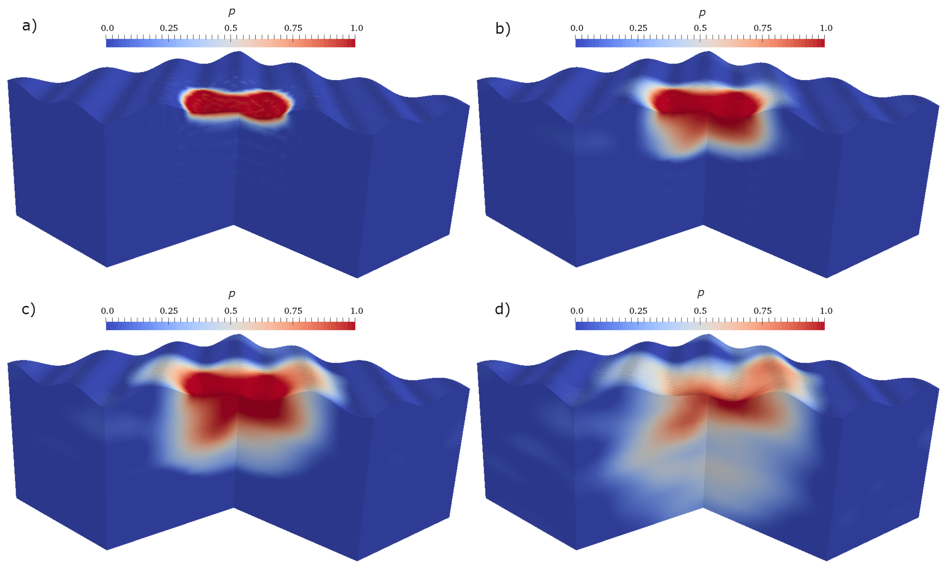
The coarse grid solution using 8 basis functions for each temperature and pressure are shown in Figure 7 and Figure 8 for four time steps. Multiscale solvers can significantly reduce the size of the system and provide accurate solutions.

These results indicate that our method is robust with respect to the contrast in the coefficient, and is able to give accurate approximate solution with a few local basis functions per each coarse neighborhood. Numerical results demonstrate fact that the infiltration process strongly affects the frozen ground.

7. Conclusions

A generalized multiscale method for solving the problem of the seepage process into permafrost soil is presented. Such kinds of problems are relevant for applied problems which involve the processes of thawing and freezing of a permafrost layer. The adaptive basis functions have been developed that take into account irregularities on discretization level for the complex geometry of the surface. The Multiphysics model was assembled based on two nonlinear problems (Richards equation and Stefan problem) for numerical implementation. We want to that our results are numerical and further studies are needed to obtain the convergence. Based on the foregoing, the proposed method has shown its efficiency both in simplified two-dimensional problems and in applied real three-dimensional cases. To demonstrate modeling potential the results of numerical calculations carried out in conditions close to the Yakutia region are presented.