
Improved Constrained k-Means Algorithm for Clustering with Domain Knowledge

1
College of Mathematics and Data Science, Minjiang University, Fuzhou 350116, China
2
College of Mathematics and Computer Science, Fuzhou University, Fuzhou 350116, China
3
School of Computer Science, Qilu University of Technology, Jinan 250353, China
*
Authors to whom correspondence should be addressed.
†
These authors contributed equally to this work.
Mathematics 2021, 9(19), 2390; https://doi.org/10.3390/math9192390
Submission received: 21 July 2021
/
Revised: 8 September 2021
/
Accepted: 16 September 2021
/
Published: 26 September 2021
(This article belongs to the Special Issue Data Analysis and Domain Knowledge)
Abstract
:Witnessing the tremendous development of machine learning technology, emerging machine learning applications impose challenges of using domain knowledge to improve the accuracy of clustering provided that clustering suffers a compromising accuracy rate despite its advantage of fast procession. In this paper, we model domain knowledge (i.e., background knowledge or side information), respecting some applications as must-link and cannot-link sets, for the sake of collaborating with k-means for better accuracy. We first propose an algorithm for constrained k-means, considering only must-links. The key idea is to consider a set of data points constrained by the must-links as a single data point with a weight equal to the weight sum of the constrained points. Then, for clustering the data points set with cannot-link, we employ minimum-weight matching to assign the data points to the existing clusters. At last, we carried out a numerical simulation to evaluate the proposed algorithms against the UCI datasets, demonstrating that our method outperforms the previous algorithms for constrained k-means as well as the traditional k-means regarding the clustering accuracy rate although with a slightly compromised practical runtime.
1. Introduction
As one of the most renowned unsupervised machine learning methods, clustering has been widely used in many research areas, including data science and natural language processing, etc. Hence, it is attracting numerous research interests from both academic and industrial communities. For many applications in machine learning and data mining involving procession of large amounts of data, there might exist a lot of unlabeled data. It would consume a lot of time and resources to manually label these data in most cases. In this context, clustering arises as it does not need labels and could appropriately preprocess the data for further usage. Moreover, researchers found that some relevant domain knowledge is useful to improve the accuracy of clustering. More generally, using the background information including domain knowledge, Wagstaff and Cardie [1] proposed semi-supervised clustering to improve the clustering performance against unlabeled data, improving the state-of-the-art accuracy rate at that time. The domain information is given in the form of must-link and cannot-link constraints in many scenarios, where the must-link constraints mean that two involved sample points must be in the same cluster during the procession of clustering; in contrast, the cannot-link constraints indicate that the two involved sample points must be in different clusters after the procession of clustering. Formally, we define must-link and cannot-link as in the following:
- Must-link: constraints specifying two sample points must be in the same cluster.
- Cannot-link: constraints specifying a set of sample points that must not be placed in the same cluster, i.e., must be placed in a manner that each of them is in a distinct cluster.
For example, assume there exist two sample points . If the two sample points are with a must-link constraint, then and must be clustered into a cluster; in contrast, if they satisfy a cannot-link then they cannot be clustered into the same cluster. Then we can formally define the constrained k-means problem as follows:
Definition 1
(The constrained k-means problem). Let be a data set in which each point is a d-dimensional real vector. In addition, we are also given a collection of must-links and a set of cannot-links . For a given integer k, the constrained k-means problem aims to divide the given data set D into k disjoint subsets such that for each must-link , u is in if and only if v is in , while for each cannot-link , u is in if and only if v is not in . Moreover, the within-cluster sum of squares is minimized as in the following:
where is the mass center of that .
1.1. Related Work
Due to the numerous applications of clustering, there exist a large number of clustering methods, such as the famous k-means algorithm based on partitioning clustering; the well-known DBSCAN algorithm based on density clustering [2] and the AGNES algorithm derived from level clustering [3]. Among the rich literature, the k-means algorithm proposed by MacQueen [4] in 1967 is one of the most prevalent clustering method. In recent years, many variants of k-means have been studied. Li et al. [5] designed approximation algorithms for the k-means problem with penalties based on seeding algorithms, and their result was demonstrated and can be extended to the k-means++ problem with the penalty version. Bi-criteria seeding algorithms were devised by Li [6] for solving the k-means problem with penalties and spherical k-means problems, improving the performance guarantees of the k-means++ algorithm for these two problems. In the more-than-50-years history after its invention, the k-means algorithm was dominantly used in many fields, such as data mining, image segmentation and information retrieval.
Observing the fact that the performance of the k-means algorithm depends on the selection of the initial centers, many k-means seeding methods have been proposed for various of k-means algorithms [7,8,9]. The k-means++ algorithm by Arthur and Vassilvitskii [7] augmented the traditional k-means algorithm with a simple randomized seeding technique, and was shown to deserve an approximation ratio of . For further improving the initial clustering centers of the k-means algorithm, Lai and Liu proposed a density-based method to determine the initial centers [9]. Later, the k-means algorithm was proposed by Bahmani et al. and was shown to perform better than k-means++ in both sequential and parallel settings [8]. In the heuristic algorithm’s side, a deterministic initialization algorithm for k-means (Dk-means) was proposed by Jothi et al., which explored a set of probable centers based on a constrained bi-partitioning approach, and achieved a remarkable convergence speed and stability [10].
The k-means algorithm is of vital importance and has a wide range of applications in many different fields. In the last century, the k-means algorithm was used by Marroquin and Girosi to solve tasks including image segmentation and the pattern classification problem [11]. More recently, the k-means algorithm was employed by Chehreghan and Abbaspour to propose a hybrid clustering algorithm that can be used to cluster high-resolution satellite images by combining with the artificial bee colony optimization method [12]. Later, the k-means algorithm was applied in multi-dimensional time series analysis, and significant progress has been made by Mashtalir et al., who combined iterative deepening time-warping technology with matrix harmonic k-means to cluster video sequences [13]. Recently, the k-means algorithm was extended by Melnykov and Zhu to cluster the skewed data [14]. For a remote sensing analysis of a canopy system, Kuo et al. [15] used the k-means algorithm and an ochre structure to demonstrate a leaf segmentation approach and the subsequent application of plane-fitting to estimate the leaf angle, demonstrating a high potential to make a significant contribution to future plant and forest research. Yuan et al. [16] analyzed the impact of four k-value selection algorithms on the convergence results of the k-means clustering algorithm and used the standard data set Iris to verify the experimental results. Ahmed et al. [17] gave a structured and synoptic overview of the k-means algorithm to overcome the shortcomings of the algorithm, and studied the latest development and effectiveness of variants of k-means algorithms. The k-means algorithm was also used in agriculture [18] and water cleaning [19].
In the above problems, the traditional k-means algorithm only paid attention to the data of the given dataset. However, in practical problems, we could have some additional domain knowledge besides the given data set itself. Such information is also useful for clustering, because they could be used to significantly improve the accuracy of clustering. This brings about the concept of constrained k-means clustering, which, to the best of our knowledge, was first addressed by Wagstaff [20]. The proposed constrained semi-supervised clustering method used background information (including domain knowledge) as constraints, such that the clustering accuracy of their algorithm outperforms the traditional k-means algorithm. Constrained k-means clustering has applications in many fields and has brought many important achievements. Cao et al. [21] incorporated constraints into k-means, such that the effectiveness of multi-view video data clustering was improved. In social media, Tang et al. [22] used constrained k-means for the classification and reviewing tasks of signed network mining for better accuracy. Later, the constrained k-means algorithm was utilized by Liu et al. [23] to solve the problem of domain adaptation, which was the first time the domain adaptation problem was re-formulated as a semi-supervised clustering problem where target labels have missing values. More recently, constrained k-means algorithm was employed by Zhang and Jin [24] to construct a blind detector for spatial modulation.
Recently, Qian et al. [25] proposed an online constrained k-means algorithm based on the novel clustering pretext task such that some instances can be learned simultaneously respecting the representations and relations. Baumann [26] proposed a binary linear programming based on the k-means approach for the constrained k-means algorithm that is better at clustering than the dual iterative local search algorithm in much shorter running time. However, it is well known that the binary linear programming cannot be used to solve large-scale problems. Therefore, we proposed an algorithm to solve the problem by employing minimum weight matching.
1.2. Our Results
In this paper, we proposed an algorithm for the constrained k-means clustering problem regarding must-link and cannot-link constraints. The contribution can be summarized as follows:
- Propose a framework to incorporate must-link and cannot-link constraints with the k-means++ algorithm;
- Devise a method to cluster the points of cannot-link via novelly employing minimum weight matching and to merge the set of data points confined by must-links as a single point;
- Carry out experiments to evaluate the practical performance of the proposed algorithms against the UCI datasets, demonstrating that our algorithms outperform the previous algorithm at a rate of 65% regarding the accuracy rate.
Note that our method deserves the advantage that it produces the clustering result with a higher accuracy, and as a price, it consumes a higher runtime than the traditional k-means algorithm.
1.3. Organization
The remainder of the paper is organized as in the following: Section 2 introduces the preliminaries and problem model; Section 3 proposes the constrained k-means clustering algorithm regarding domain knowledge as side information; Section 4 introduces the method for evaluating the performance of the algorithm, and demonstrates experimental results comparing our constrained k-means with other baselines including the traditional k-means algorithm; Section 5 concludes this paper.
2. Preliminaries and Problem Statement
In this section, we mainly introduce the definition of pair-wise constraints. Then we give a figure to show the shortcomings of the constrained k-means clustering algorithm that is proposed by Wagstaff [20]. After that, we propose an improved method to improve the result of clustering.
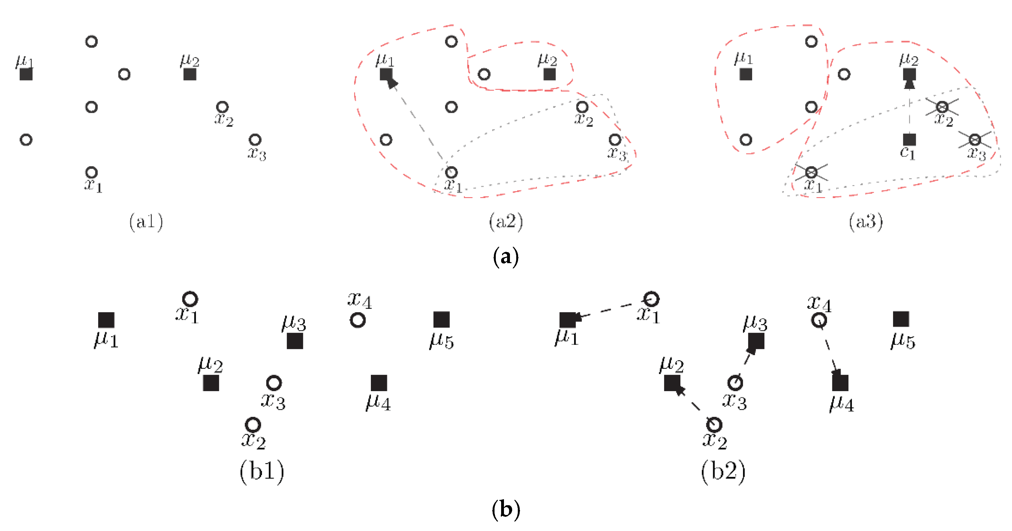
We use Figure 1 to demonstrate the procession of the previous constrained k-means algorithm [20], and our algorithm deald with must-link and cannot-link constraints, in which Figure 1a shows the must-link constraint and Figure 1b is the cannot-link constraint.
In Figure 1a, there are a set of clustering centers and a set of sample points . Since the four simple points in V must satisfy the must-link constraints, then if is assigned to , must also be allocated to ; otherwise, if is assigned to , then it means will be allotted to . Therefore, the four sample points can be assigned to (or ) at the same time. Let be the distance between a sample point and a clustering . Let be the sum distance between a clustering and a set of sample points . When using the constrained k-means in [20], the four points must be allotted to if is firstly selected [20], since . However, that is not the best result of clustering. Due to , the four points should be assigned to to incorporate an optimum solution. Therefore, we propose a new method to deal with a must-link set to prevent the above inaccuracy. In our algorithm, we first calculate the center point x of the set of sample points V, and then determine whether the center x is assigned to or according to the distance between the center x and or .
Figure 1b has a set of clustering mass centers and a set of sample points , in which each pair of sample points in V must satisfy the cannot-link constraints. Hence, there must exist at least four clusters, so that the sample points can be divided into different clustering centers. Let be the distance between a clustering and a sample point . Then obviously can be calculated for any pair and . Thus, we can use the bipartite minimum weight matching between the two vertex sets U and V to solve the cannot-link constraint. The definition ofthe minimum-weight matching can be described as follows:
Definition 2
([27])). Let be a bipartite graph and let be the weight of the edges. For any subset F of E, denote as the weight of F. We say M is a match if and only if M is a set of disjoint edges subset of E. The aim of minimum-weight matching is to find a matching M covering all vertices of U or V, such that attains the minimum.
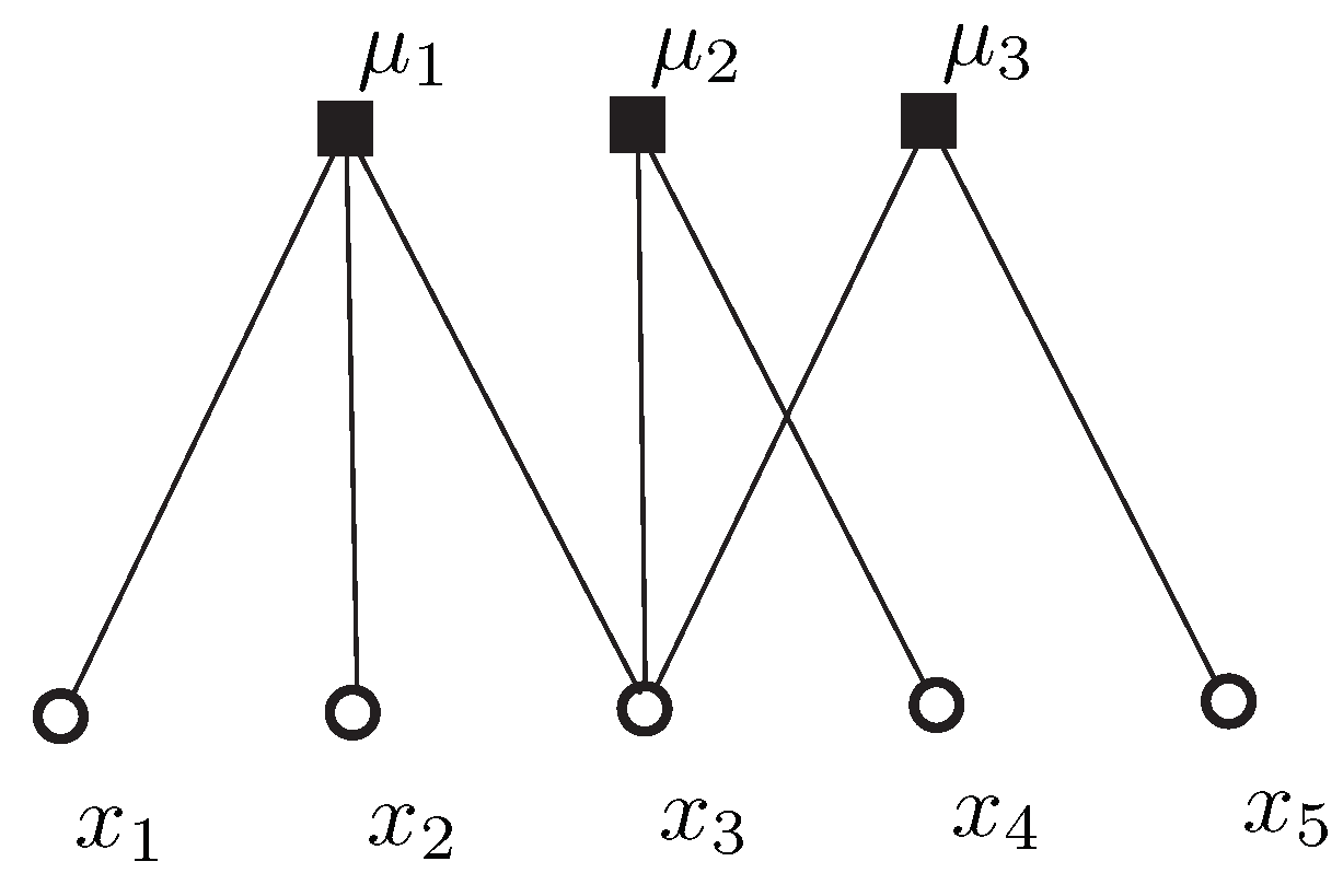
Figure 2 gives a more detailed explanation about Definition 2, in which there exist two types of sample point sets and . Then we can find that is a matching and is not matching.
Let and be a set of sample points and a family of cluster centers, respectively. Let be the distance between cluster and sample point . Let if be assigned to , otherwise set for is not clustered to . Then the integer linear programming for the minimum weight matching can be described as follows:
The first constraint means each cluster contains at most one sample point; the second means each sample point must be clustered to a cluster.
As a well-known combinatorial optimization problem, the minimum weight unbalance perfect matching problem already has known efficient algorithms in the existing literature:
Lemma 1
([28]). Let G be a given graph with two partitions U and V. Assume that and there are m edges in G. Then the minimum weight unbalance perfect matching of G can be found within a runtime of .
3. Constrained k-Means Clustering Algorithm with Incidental Information
In this section, for the constrained k-means problem (CKM) that is proposed by Wagstaff et al. [20], we propose an algorithm to solve this problem. Though there exists an algorithm that has been proposed in [20], a bad cluster may be found for some sample points, which satisfies the must-link constraints since the algorithm does not consider the domain knowledge of the given dataset. Therefore, we propose an algorithm to deal with the must-link constraint based on known domain knowledge. For a set of sample points with the cannot-link constraints, we solve it by using the minimum weight matching that is different to [20].
Given a set of sample points . Let be the initial set of clusters. If a few sample points in V satisfy the must-link constraints, then these sample points must be divided into a group based on the transitivity of all constraints. Based on the above fact, we can compute the center of the set to replace the attribute value for all sample points of the set. Note that, when the sample point is allocated to a cluster, each sample point is allocated to the same cluster for the set. When a few sample points are with the cannot-link constraints, we can put these sample points into a set , then all sample points of must be divided into different clusters based on the definition of cannot-link. Hence, there must exist , such that the distance between sample points and cluster can be employed as the attribute value of . Before executing the main algorithm, we shall firstly preprocess the data points incident to the must-link and cannot-link constraints.
The key idea of our algorithm is to incorporate must-link and cannot-link constraints to the k-means++ framework. In general, we shall merge the set of data points confined by must-links as a single point and cluster the points of cannot-link separately after clustering other data points via employing minimum weight matching. Therefore, the algorithm mainly consists of iterations, where each iteration is composed of the three steps as follows: (1) embed the must-link constraints into the data points by merging the set of points confined by must-links as one point but with a weight equal to their weight sum; (2) employ the traditional k-means++ algorithm against the remaining data points, including the merged data points for must-link but excluding the points incident to cannot-links; (3) use the bipartite minimum-weight matching method to assign data points incident to cannot-link constraints to the clusters. The above steps will be repeated until the within-cluster sum of squares only decrease smaller than a given threshold . Then the formal layout of the algorithm is as described in Algorithm 1.
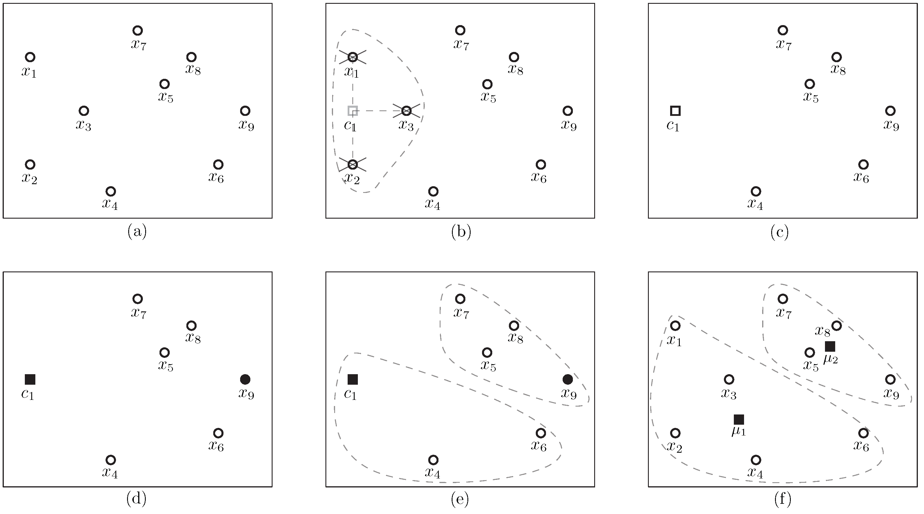
We illustrate an example of executing Algorithm 1 as in Figure 3. Figure 3a is the given data set , in which the must-link constraint set is and the cannot-link constraint sets are and . The first step is to compute the mass center for the data points incident to must-link constraints as in Figure 3b, in which is the center between and and we use to replace and as in Figure 3c. After that, we randomly select clusters (Figure 3d) that are and . The clustering results are as shown in Figure 3e in which and , where . Later, recalculate a center for each , obtaining the centers and for and , respectively (Figure 3f). Then by the termination criteria, the clusters remain unchanged after re-assignment of the points to their nearest centers. Hence, the clusters are and .
| Algorithm 1 Constrained k-means clustering using domain information. |
| Input: A data set , must-link constraints , cannot-link constraints , a positive integer k; Output: A collection of k clusters . 1: Use the k-center algorithm to select as the initial cluster centers; 2: Set; 3: While cluster centers change do 4: For each set of must-link constraints do 5: Compute mass center sample of the set; 6: Assign all samples of the set to the nearest ; /* Adding all samples of the set to */ 7: EndFor 8: For do 9: Compute the distance between point and cluster center ; 10: EndFor 11: Assign remaining points to their nearest , except those incident to cannot-links; 12: For each set of cannot-link constraint do 13: Assign each point to the appropriate cluster via minimum weight matching; 14: EndFor 15: Compute the cluster center of ; 16: EndWhile 17: Return . |
4. Experimental Evaluation
In this section, we evaluate our improved constrained k-means algorithm (ICM) via comparing to baselines, including traditional k-means (TM) and constrained k-means (CM), respecting the external indicator’s Adjusted Rand Index (ARI). The experiments were run against datasets from the public UCI datasets. All the algorithms were implemented with Python 3.7, and the figures were drawn using matplotlib. For the external indicators ARI, we directly use the metrics.adjusted_rand_score method within sklearn library in Python to automatically calculate the clustering result. The experiments were carried out on a Win 10 platform with Intel Core i5-6200U CPU, 8.0G RAM.
4.1. Evaluation Approaches
In this subsection, we propose a method to evaluate the performance of our algorithm via comparing to other baselines. We adopt the performance metrics of clustering, which is known as validity metrics and is similar to the metrics of measuring the performance of supervised learning, to measure the quality of clustering results for our algorithm and the baseline algorithms in comparison.
For evaluating the clustering results, we use the following metrics for measurement: (1) the similarity for all sample points in the same cluster; (2) the difference among all sample points located in different clusters. The aim is such that higher similarity within cluster and higher difference among clusters indicate better clustering results. For the performance metric of clustering, there exists two types as follows: the first is an external indicator, which is obtained by comparing the experimental results of the cluster with a reference model; the other is an internal indicator that directly uses the clustering results to examine and without any other reference models. In this paper, the external indicators are used to evaluate the performance metric of clustering of our algorithm in a similar manner as in paper [20].
When the external indicators are used to evaluate our algorithm, an external reference model needs to be determined in advance. Let be the given dataset, and be the set of cluster centers that are produced by using the external reference model and be also a set of clusters produced by an algorithm. We use as the cluster center of U and as . Then each element of and each element of U can be matched as shown in the following:
where a is the length of , where is a set of paired sample points, and and are clustered to the same cluster class in U and for each paired sample points ; Then b is also the length of a set of paired sample points , in which each paired sample points satisfies and are classified into the same cluster class in U while into different clusters in . Similarly, c and d are respectively the lengths of and . Furthermore, means and belong to two clusters for U and one cluster for . shows that and must locate in different clusters of U and . Hence, for each paired sample points, it only belongs to one of and , such that we have the following formulation:
The Rand Index (RI) has been an indicator to evaluate the clustering results since 1997 due to Milligan and Cooper [29,30]. For a given dataset, we can use the RI to measure the consistency between the clustering results and the external reference model. Note that the value range of the RI is . When , we obtain possibly the best clustering effect. In contrast, if , the clustering effect reaches the worst bottom. Formally, the RI can be defined as follows:
However, the coefficient value of the RI is obviously not a constant tending to zero. Therefore, we need the coefficient value of the RI such that the RI can also work when the coefficient value of the RI tends to zero. Hence, the Adjusted Rand Index (ARI) was proposed and its range is [31]. Meanwhile, the clustering effect is more consistent with the reference model when the value is larger. In our paper, ARI is used to calculate accuracy for all of our experiments, which is formally defined as follows:
4.2. Experimental Dataset and Statistics Information
For each dataset, we use the result of 20 iterations as the final value in our experiments, which is obtained through the following steps: (1) Use Python to compute a value in each iteration; (2) calculate the ARI of each value; (3) take the average of all ARIs. Note that there exist a certain number of new constraints that are obtained after each iterate and will be added to the subsequent algorithm process for further procession.
In this paper, all datasets were selected from the UCI datasets, where each dataset contains at least one sample. Each sample contains a number of attributes, one of which may be a decision attribute. First of all, note that there may be some same or different decision attributes for different samples in one dataset. Second, the number of decision attributes is the same as the number of cluster classes in the dataset. In our algorithm, the must-link and cannot-link constraints are crucial, and they can be generated by the decision attributes, in which each must-link constraint comes from two samples that are with the same decision attribute; while each cannot-link constraint is also generated by two samples that have different decision attributes.
4.3. Comparison of Practical Performance
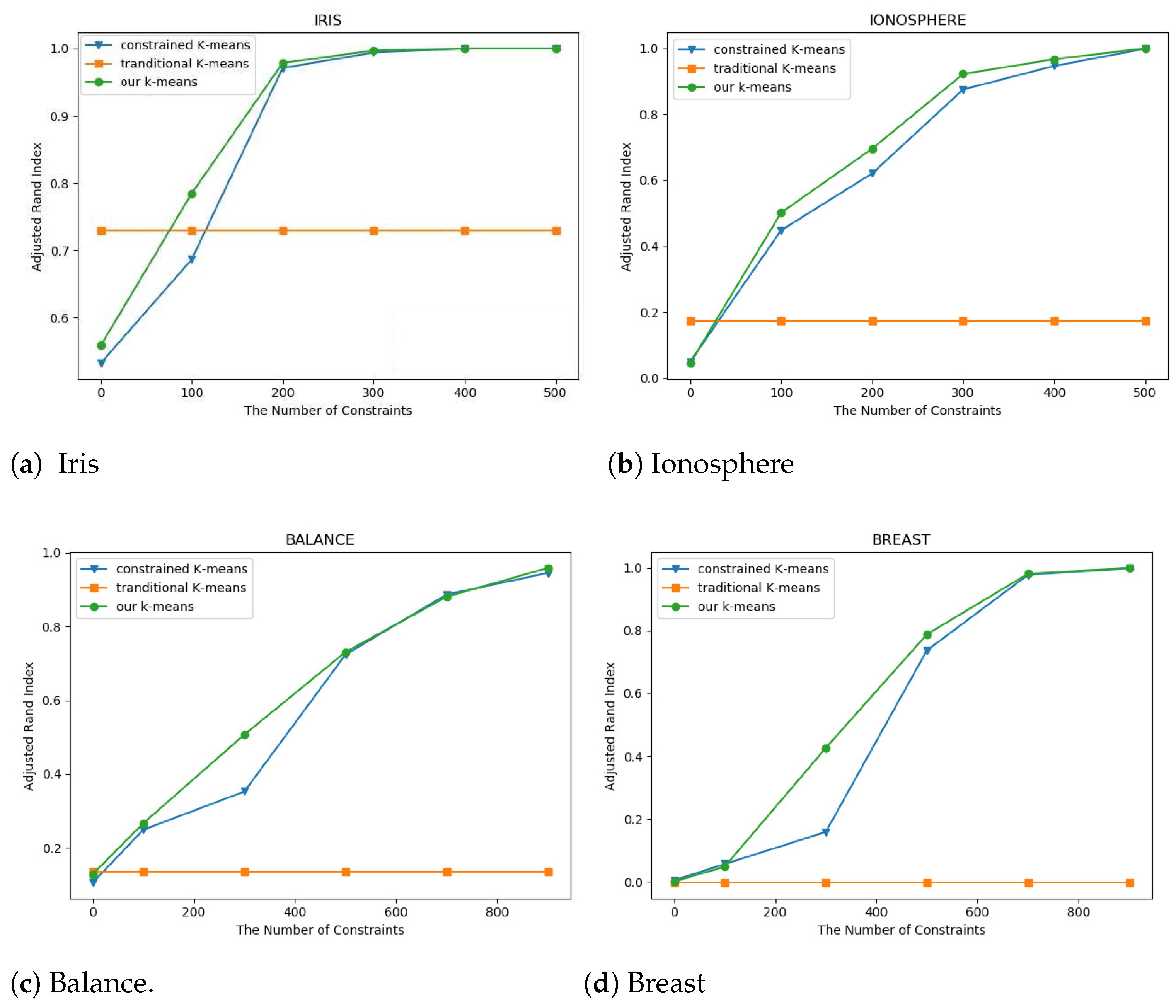
The first data set selected was Iris, which has 150 samples and 5 attributes, and will finally form 3 clusters. The results were demonstrated in Table 1 and Figure 4a. The number of constraints in the experiments increased from 100 to 500 by 100 at one step. For the constrained k-means algorithm and the improved constrained k-means algorithm, the accuracy of clustering is gradually increasing along the increment of the number of constraints. The reason is that more constraints indicate more information, which leads to better accuracy. The ARI of constrained k-means is always no more than the ARI of the improved constrained k-means when the number of constraints is less than 400. When the number of constraints is larger than 400, the ARI is identically 1 for both the constrained k-means algorithm and our improved constrained k-means algorithm. Hence, the accuracy of clustering attains 1 for both the two algorithms when the number of constraints is larger than 400 and enough domain knowledge is provided. The ARI of the traditional k-means algorithm is always 0.73023, which does not change with the number of constraints.
In the second dataset, Ionosphere, as illustrated in Table 2 and Figure 4b, the number of samples and the number of attributes are fixed at 351 and 34, respectively. After clustering, two cluster classes are eventually formed. The number of constraints of each group of Ionosphere is the same as that of Iris. It is very obvious that the ARI of the k-means algorithm is also always 0.17284. When the number of constraints is 100, the ARI of the constrained k-means is 0.44799 and it is 0.50131 for the improved constrained k-means. The ARIs are 0.99817 and 0.99908 for the constrained k-means and the improved constrained k-means, receptively. The accuracy of clustering for the improved constrained k-means is always larger than the constrained k-means that accords with our theoretical analysis.
The Balance dataset is our third selection dataset with 625 samples and 5 attributes, and eventually, 3 clusters will be found. Table 3 and Figure 4c show the experimental results. The minimum number of constraints is 100 and the maximum is 900, and there exist five groups in our experiments. For the k-means algorithm, 0.13234 is its ARI value regardless of the number of constraints. When the number of constraints is 100, the ARI value of the constrained k-means is 0.24879 and the ARI value is 0.26650 for the improved constrained k-means, is true. When the number of constraints increases to 900, the ARI of the constrained k-means (0.94483) is also less than the improved constrained k-means (0.95854).
The fourth dataset we picked is Breast (Table 4 and Figure 4d). For the dataset, the numbers of samples and attributes are, respectively, 682 and 11 in our experiments, and there exist five cluster classes in total. The number of constraints for the Breast dataset is the same as the Balance dataset in each group experiment. The ARI of the traditional k-means is always less than 0, which is −0.00268, which means the clustering effect is very poor. When the number of constraints is 100, the ARI of the constrained k-means is 0.05636 and larger than the ARI of the improved constrained k-means (0.04795). The ARI of the constrained k-means is always less than the improved constrained k-means when the number of constraints is not less than 300. Importantly, the ART of the improved constrained k-means is very close to 1, with only a 0.0003 difference.
From the above four tables and four figures, we find that the ARI value increases with the number of constraints for the constrained k-means and the improved constrained k-means. That is, the clustering effect becomes better with the increase in constraints. The ARI of the improved constrained k-means algorithm is larger than the constrained k-means algorithm, so our algorithm can obtain better clustering results. Hence, the improved constrained k-means algorithm that we propose in this paper is successful.
4.4. Comparison of Runtime
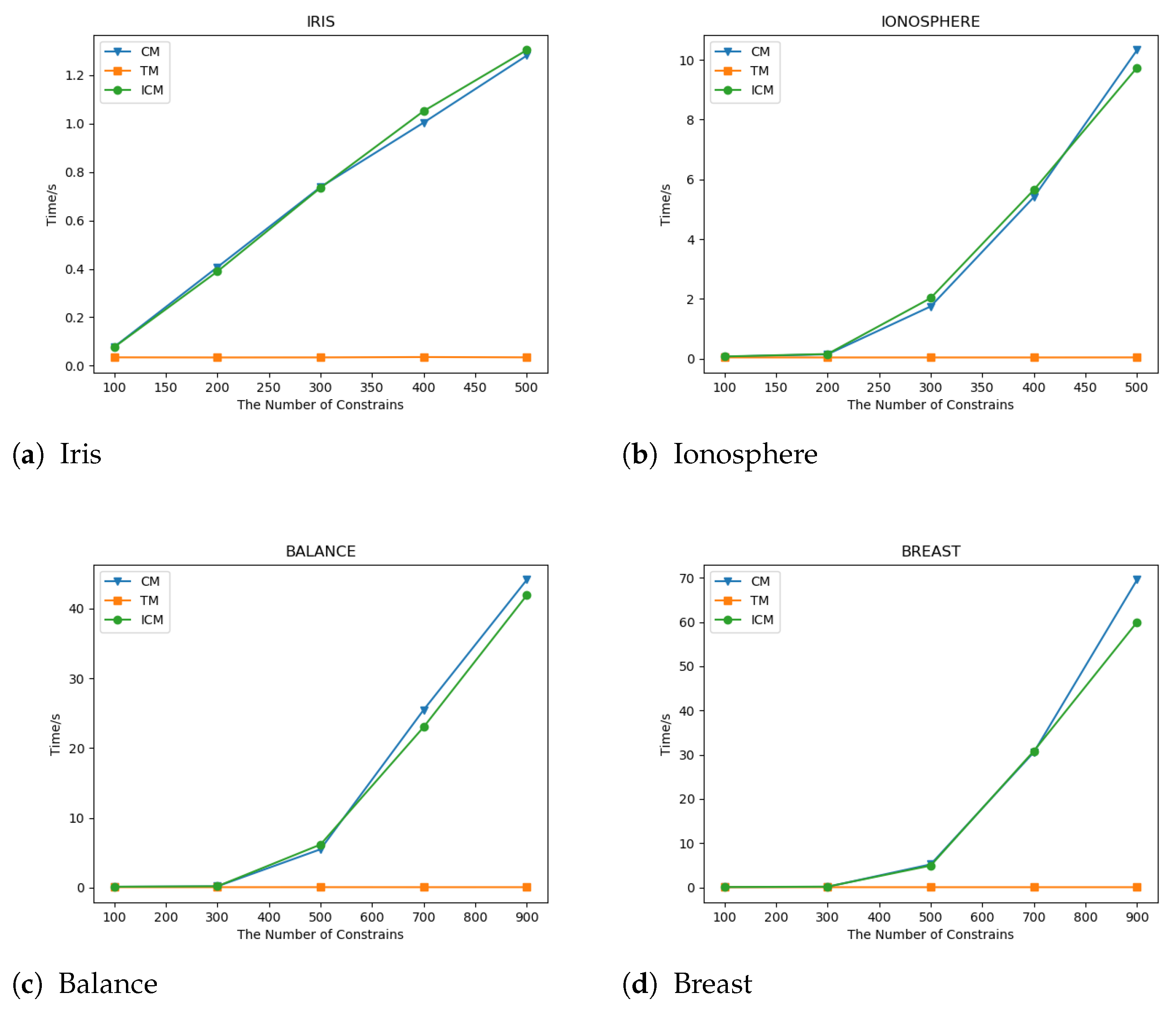
Figure 5a demonstrates the runtimes of CM, TM, and ICM on Iris. When the number of constraints is not more than 320, the runtime of ICM is less than CM. Contrarily, the runtime of CM is smaller than ICM if the number of constraints is larger than 320. The runtime of TM is almost a straight line, which means the number of constraints has little effect on the runtime of TM, and the difference between the maximum and the minimum runtimes is 0.0018.
The runtimes of CM, TM, and ICM on Ionosphere are shown in Figure 5b. The runtimes of CM and ICM growth are slow when the number of constraints is not larger than 200, and after that, the runtime grows faster as the number of constraints increases. What is more, the runtime of CM is smaller than ICM when the number of constraints is less than 450. When the number of constraints increases to more than 450, the runtime of CM is larger than ICM. This means that our algorithm can be used to solve large-scale problems with more accurate results and a shorter time.
For Balance, the runtimes of CM, TM, and ICM are shown in Figure 5c. When the number of constraints is not larger than 500, the runtime of CM is smaller than ICM, and the difference between the runtimes of CM and ICM increases with the number of constraints. However, the difference is very small and is less than 1. Once the number of constraints exceeds 700, the runtime of ICM is smaller than CM, and the difference grows as the number of constraints increases, and the difference is 2.4629 when the number of constraints is 700.
The runtimes of CM, TM, and ICM on the Breast are shown in Figure 5d. When the number of constraints is less than 700, the gap between the runtimes of CM and ICM is very small and is less than 1. When the number of constraints exceeds 700, the runtime of CM is larger than ICM, and the gap between the two runtimes increases with the increase in the number of constraints.
5. Conclusions
In this paper, we first proposed a model for clustering with must-link and cannot-link constraints. Then, an algorithm incorporating side information were proposed to solve the constrained k-means clustering problem. The key idea of the algorithm is to repeat the following procession until satisfactory clustering of the data points is obtained: firstly, compute a mass center for the data points that are constrained by the must-links; secondly, collaborate the clustering against the unconstrained data as well as the must-link constrained data, while ignoring the data points involved by the cannot-links; and thirdly, to transform the task into the problem of finding a minimum weight matching in a bipartite graph regarding the cannot-link constraints. Lastly, we carried out numerical experiments against four UCI datasets: Iris, Ionosphere, Balance and Breast, demonstrating the practical gain of our algorithm compared with traditional k-means as well as the constrained k-means proposed by Wagstaff [20].
Author Contributions
Conceptualization, P.H. and L.G.; methodology, P.Y. and P.H.; software, Z.H.; validation, P.H.; formal analysis, P.Y.; investigation, P.Y.; resources, H.P.; data curation, H.P.; writing—original draft preparation, P.H.; writing—review and editing, P.H. and P.Y.; visualization, P.H. and P.Y.; supervision, L.G.; project administration, L.G.; funding acquisition, P.H. and L.G. All authors have read and agreed to the published version of the manuscript.
Funding
This research was funded by the Natural Science Foundation of China (No. 61772005), Natural Science Foundation of Fujian Province (No. 2020J01845) and Educational Research Project for Young and Middle-aged Teachers of Fujian Provincial Department of Education (No. JAT190613).
Institutional Review Board Statement
Not applicable.
Informed Consent Statement
Not applicable.
Data Availability Statement
Not applicable.
Acknowledgments
A preliminary version [32] of part of this paper has appeared in Proceedings of the 10th International Symposium on Parallel Architectures, Algorithms and Programming (PAAP 2019).
Conflicts of Interest
The authors declare no conflict of interest.
References
- Wagstaff, K.; Cardie, C. Clustering with instance-level constraints. AAAI/IAAI 2000, 1097, 577–584. [Google Scholar]
- Ester, M.; Kriegel, H.; Sander, J.; Xu, X. A Density-Based Algorithm for Discovering Clusters in Large Spatial Databases with Noise. In Proceedings of the Second International Conference on Knowledge Discovery and Data Mining (KDD-96), Portland, OR, USA, 2–4 August 1996; Simoudis, E., Han, J., Fayyad, U.M., Eds.; AAAI Press: Palo Alto, CA, USA, 1996; pp. 226–231. [Google Scholar]
- Sobczak, G.; Pikula, M.; Sydow, M. AGNES: A Novel Algorithm for Visualising Diversified Graphical Entity Summarisations on Knowledge Graphs. In Proceedings of the Foundations of Intelligent Systems-20th International Symposium, ISMIS 2012, Macau, China, 4–7 December 2012; Chen, L., Felfernig, A., Liu, J., Ras, Z.W., Eds.; Lecture Notes in Computer Science. Springer: Berlin/Heidelberg, Germany, 2012; Volume 7661, pp. 182–191. [Google Scholar] [CrossRef]
- MacQueen, J. Some methods for classification and analysis of multivariate observations. In Proceedings of the Fifth Berkeley Symposium on Mathematical Statistics and Probability, Oakland, CA, USA, 11–18 July 1967; Volume 1, pp. 281–297. [Google Scholar]
- Li, M.; Xu, D.; Yue, J.; Zhang, D.; Zhang, P. The seeding algorithm for k-means problem with penalties. J. Comb. Optim. 2020, 39, 15–32. [Google Scholar] [CrossRef]
- Li, M. The bi-criteria seeding algorithms for two variants of k-means problem. J. Comb. Optim. 2020, 1–12. [Google Scholar] [CrossRef]
- Arthur, D.; Vassilvitskii, S. k-means++: The advantages of careful seeding. In Proceedings of the Eighteenth Annual ACM-SIAM Symposium on Discrete Algorithms, New Orleans, LA, USA, 7–9 January 2007; Society for Industrial and Applied Mathematics: Philadelphia, PA, USA, 2007; pp. 1027–1035. [Google Scholar]
- Bahmani, B.; Moseley, B.; Vattani, A.; Kumar, R.; Vassilvitskii, S. Scalable k-means++. Proc. VLDB Endow. 2012, 5, 622–633. [Google Scholar] [CrossRef]
- Lai, Y.; Liu, J. Optimization study on initial center of K-means algorithm. Comput. Eng. Appl. 2008, 44, 147–149. [Google Scholar]
- Jothi, R.; Mohanty, S.K.; Ojha, A. DK-means: A deterministic k-means clustering algorithm for gene expression analysis. Pattern Anal. Appl. 2019, 22, 649–667. [Google Scholar] [CrossRef]
- Marroquin, J.L.; Girosi, F. Some Extensions of the k-Means Algorithm for Image Segmentation and Pattern Classification; Technical Report; Massachusetts Inst of Tech Cambridge Artificial Intelligence Lab.: Cambridge, MA, USA, 1993. [Google Scholar]
- Chehreghan, A.; Abbaspour, R.A. An improvement on the clustering of high-resolution satellite images using a hybrid algorithm. J. Indian Soc. Remote Sens. 2017, 45, 579–590. [Google Scholar] [CrossRef]
- Mashtalir, S.; Stolbovyi, M.; Yakovlev, S. Clustering Video Sequences by the Method of Harmonic k-Means. Cybern. Syst. Anal. 2019, 55, 200–206. [Google Scholar] [CrossRef]
- Melnykov, V.; Zhu, X. An extension of the K-means algorithm to clustering skewed data. Comput. Stat. 2019, 34, 373–394. [Google Scholar] [CrossRef]
- Kuo, K.; Itakura, K.; Hosoi, F. Leaf Segmentation Based on k-Means Algorithm to Obtain Leaf Angle Distribution Using Terrestrial LiDAR. Remote Sens. 2019, 11, 2536. [Google Scholar] [CrossRef] [Green Version]
- Yuan, C.; Yang, H. Research on K-value selection method of K-means clustering algorithm. J 2019, 2, 226–235. [Google Scholar] [CrossRef] [Green Version]
- Ahmed, M.; Seraj, R.; Islam, S.M.S. The k-means algorithm: A comprehensive survey and performance evaluation. Electronics 2020, 9, 1295. [Google Scholar] [CrossRef]
- Aldino, A.; Darwis, D.; Prastowo, A.; Sujana, C. Implementation of K-means algorithm for clustering corn planting feasibility area in south lampung regency. J. Phys. Conf. Ser. 2021, 1751, 012038. [Google Scholar] [CrossRef]
- Windarto, A.P.; Siregar, M.N.H.; Suharso, W.; Fachri, B.; Supriyatna, A.; Carolina, I.; Efendi, Y.; Toresa, D. Analysis of the K-Means Algorithm on Clean Water Customers Based on the Province. J. Phys. Conf. Ser. 2019, 1255, 012001. [Google Scholar] [CrossRef] [Green Version]
- Wagstaff, K.; Cardie, C.; Rogers, S.; Schrödl, S. Constrained k-Means Clustering with Background Knowledge; ICML: Williamstown, MA, USA, 2001; Volume 1, pp. 577–584. [Google Scholar]
- Cao, X.; Zhang, C.; Zhou, C.; Fu, H.; Foroosh, H. Constrained multi-view video face clustering. IEEE Trans. Image Process. 2015, 24, 4381–4393. [Google Scholar] [CrossRef]
- Tang, J.; Chang, Y.; Aggarwal, C.; Liu, H. A survey of signed network mining in social media. ACM Comput. Surv. (CSUR) 2016, 49, 42. [Google Scholar] [CrossRef]
- Liu, H.; Shao, M.; Ding, Z.; Fu, Y. Structure-preserved unsupervised domain adaptation. IEEE Trans. Knowl. Data Eng. 2018, 31, 799–812. [Google Scholar] [CrossRef]
- Zhang, L.; Jin, M. A Constrained Clustering-Based Blind Detector for Spatial Modulation. IEEE Commun. Lett. 2019. [Google Scholar] [CrossRef]
- Qian, Q.; Xu, Y.; Hu, J.; Li, H.; Jin, R. Unsupervised Visual Representation Learning by Online Constrained K-Means. arXiv 2021, arXiv:2105.11527. [Google Scholar]
- Baumann, P. A Binary Linear Programming-Based K-Means Algorithm For Clustering with Must-Link and Cannot-Link Constraints. In Proceedings of the IEEE International Conference on Industrial Engineering and Engineering Management, IEEM 2020, Singapore, 14–17 December 2020; pp. 324–328. [Google Scholar] [CrossRef]
- Edmonds, J. Maximum matching and a polyhedron with 0, 1-vertices. J. Res. Natl. Bur. Stand. B 1965, 69, 55–56. [Google Scholar] [CrossRef]
- Schrijver, A. Combinatorial Optimization: Polyhedra and Efficiency; Springer Science & Business Media: Berlin, Germany, 2003; Volume 24. [Google Scholar]
- Milligan, G.W.; Cooper, M.C. A study of the comparability of external criteria for hierarchical cluster analysis. Multivar. Behav. Res. 1986, 21, 441–458. [Google Scholar] [CrossRef]
- Rand, W.M. Objective criteria for the evaluation of clustering methods. J. Am. Stat. Assoc. 1971, 66, 846–850. [Google Scholar] [CrossRef]
- Hubert, L.; Arabie, P. Comparing partitions. J. Classif. 1985, 2, 193–218. [Google Scholar] [CrossRef]
- Hao, Z.; Guo, L.; Yao, P.; Huang, P.; Peng, H. Efficient Algorithms for Constrained Clustering with Side Information. In Proceedings of the Parallel Architectures, Algorithms and Programming-10th International Symposium, PAAP 2019, Guangzhou, China, 12–14 December 2019; Revised Selected Papers. Shen, H., Sang, Y., Eds.; Communications in Computer and Information Science. Springer: Berlin/Heidelberg, Germany, 2019; Volume 1163, pp. 275–286. [Google Scholar] [CrossRef]
Figure 1.
Examples of processing must-links and cannot-links. (a) Must-link examples. (a1) is the original graph with the must-link set
and the mass clusters μ1 and μ2. (a2) is a possibly solution produced by [20] while (a3) is the solution of our algorithm. (b) A cannot-link example. (b1) A cannot-link set with four clustering centers ; (b2) an assignment of the points in the cannot-link set to the clusters.

Figure 2.
An example for Definition 2, where it contains two types of sample point sets and .

Figure 3.
An example of executing Algorithm 1: (a) the set of data points; (b) Execution for must-links where c represents the must-link set as in (c); (d) the two centers selected; (e) the clustering results; (f) the calculated means according to the clustering.
Figure 3.
An example of executing Algorithm 1: (a) the set of data points; (b) Execution for must-links where c represents the must-link set as in (c); (d) the two centers selected; (e) the clustering results; (f) the calculated means according to the clustering.

Figure 4.
Comparison of the Adjusted Rand Index.

Figure 5.
Runtime comparison of CM, TM and ICM.


Table 1.
Comparison of Adjusted Rand Index on dataset Iris.
| The Number of Constraints | 100 | 200 | 300 | 400 | 500 |
|---|---|---|---|---|---|
| CM | 0.68669 | 0.97119 | 0.99399 | 1.00000 | 1.00000 |
| TM | 0.73023 | 0.73023 | 0.73023 | 0.73023 | 0.73023 |
| ICM | 0.78485 | 0.97860 | 0.99699 | 1.00000 | 1.00000 |
Table 2.
Comparison of Adjusted Rand Index on dataset Ionosphere.
| The Number of Constraints | 100 | 200 | 300 | 400 | 500 |
|---|---|---|---|---|---|
| CM | 0.44799 | 0.62021 | 0.87489 | 0.94606 | 0.99817 |
| TM | 0.17284 | 0.17284 | 0.17284 | 0.17284 | 0.17284 |
| ICM | 0.50131 | 0.69528 | 0.92172 | 0.96657 | 0.99908 |
Table 3.
Comparison of Adjusted Rand Index on dataset Balance.
| The Number of Constraints | 100 | 300 | 500 | 700 | 900 |
|---|---|---|---|---|---|
| CM | 0.24879 | 0.35256 | 0.72374 | 0.88657 | 0.94483 |
| TM | 0.13234 | 0.13234 | 0.13234 | 0.13234 | 0.13234 |
| ICM | 0.26650 | 0.50679 | 0.73070 | 0.88045 | 0.95854 |
Table 4.
Comparison of Adjusted Rand Index on dataset Breast.
| The Number of Constraints | 100 | 300 | 500 | 700 | 900 |
|---|---|---|---|---|---|
| CM | 0.05636 | 0.15859 | 0.73693 | 0.97761 | 0.99873 |
| TM | −0.00268 | −0.00268 | −0.00268 | −0.00268 | −0.00268 |
| ICM | 0.04795 | 0.42613 | 0.78812 | 0.98097 | 0.99970 |
Publisher’s Note: MDPI stays neutral with regard to jurisdictional claims in published maps and institutional affiliations. |
© 2021 by the authors. Licensee MDPI, Basel, Switzerland. This article is an open access article distributed under the terms and conditions of the Creative Commons Attribution (CC BY) license (https://creativecommons.org/licenses/by/4.0/).
Share and Cite
MDPI and ACS Style
Huang, P.; Yao, P.; Hao, Z.; Peng, H.; Guo, L. Improved Constrained k-Means Algorithm for Clustering with Domain Knowledge. Mathematics 2021, 9, 2390. https://doi.org/10.3390/math9192390
AMA Style
Huang P, Yao P, Hao Z, Peng H, Guo L. Improved Constrained k-Means Algorithm for Clustering with Domain Knowledge. Mathematics. 2021; 9(19):2390. https://doi.org/10.3390/math9192390
Chicago/Turabian StyleHuang, Peihuang, Pei Yao, Zhendong Hao, Huihong Peng, and Longkun Guo. 2021. "Improved Constrained k-Means Algorithm for Clustering with Domain Knowledge" Mathematics 9, no. 19: 2390. https://doi.org/10.3390/math9192390
Note that from the first issue of 2016, this journal uses article numbers instead of page numbers. See further details here.