1. Introduction
Optimal control may be characterized as the determination of inputs to a dynamical system that optimize an objective functional while satisfying all constraints of the system [
1]. In epidemiology, optimal control plays an important role in finding from among the available strategies the most effective strategy to reduce the infection rate to an acceptable level, while minimizing the cost of therapeutic or preventive measures that control the disease progression.
Two major mathematical results in the theory of optimal control are Pontryagin’s maximum principle and the Arrow theorem. In some cases, these are sufficient to determine optimal solutions. For example, Pontryagin’s principle is applied to a mathematical model of dengue transmission in [
2] to determine optimal interventions. However, more realistic models often do not satisfy the hypotheses required for theoretical analysis. In such cases, various numerical methods are used to estimate optimal controls. For example, the authors in [
3] investigate the measures against dengue fever by using mathematical modeling and numerical methods of optimal control. Optimal control theory and nonlinear programming approaches are applied to Dengue epidemic models [
4]. An enumerative numerical method for finding near-optimal controls for SIS epidemic model under treatment and vaccination is developed by [
5].
There are several different general approaches to numerical optimization. Descent methods (such as Newton iteration or conjugate gradient) iteratively identify “best” search directions based on local properties in the neighborhood of the current solution. On the other hand, enumerative methods such as dynamic programming conduct a systematic search throughout a subspace of possible solutions. Finally, Monte Carlo methods wander randomly through solution space, computing sample solutions and disproportionately sampling regions that have better solutions. These three general approaches all have their advantages and disadvantages. Descent methods will converge rapidly to a local optimum, but have no way of determining whether the local optimum is globally the best solution. Enumerative methods must usually be limited to a relatively small subset of possible solutions in order to be practically computable. Monte Carlo methods both explore a relatively extensive subregion of solution space and can avoid inferior local optima to some extent, but are still unable to accomplish a truly global search and are not good at settling in to a precise local optimum.
The strengths and deficiencies of each of the above methods to some extent compensate for each other. This indicates that an algorithm that combines the three approaches together may possibly combine the strengths and avoid the weaknesses of each individual method. The natural way to do this is to start with an enumerative method that identifies a favorable starting point for Monte Carlo; then, use Monte Carlo to identify the most promising local optimum; then, apply a descent method to home in on the exact local optimum. In this paper, we present an algorithm that follows this schema, and apply it to a detailed model of corona virus disease 19 (COVID-19) transmission [
6] that is based on practical data from Houston, Texas, USA. We assume that testing and distancing are the two available control means, and vary parameters in the objective function.
The organization of the paper is as follows:
Section 2 reviews previous work in the area of control of COVID-19 through the use of non-pharmaceutical measures.
Section 3 describes the multicompartment system model.
Section 4 introduces controls into the model and provides justification. Theoretical results from optimal control theory are briefly recalled in
Section 5.
Section 6 formulates and justifies the objective function, while
Section 7 analyzes the local optimality conditions for our model.
Section 8 describes the three-stage algorithm in detail, while
Section 9 presents and discusses the results obtained from three variants of the algorithm.
Section 10 summarizes the research and draws general conclusions.
2. Previous Work
As of 2021, ongoing intensive efforts are being made to stop the spread of COVID-19 and eradicate it as soon as possible. Much research has dealt with evaluating the efficacy of various non-pharmaceutical measures applied to reduce the virus propagation. Several studies are based on geographical data from various regions. Mitigation which slows down the epidemic spread, and suppression which reverses epidemic growth and reduces case numbers to low levels are studied in [
7] for the UK and the US. The authors in [
8] estimate the effect of non-pharmaceutical interventions across 11 European countries beginning from the start of the epidemic in February 2020 until 4 May 2020. The authors in [
9] model the control of COVID-19 transmission in Australia by means of intervention strategies such as restrictions on international air travel, isolation, home quarantine, social distancing and school closures, while the authors in [
10] model the application of similar measures in Wuhan province over December 2019 and February 2020. In [
11], a dynamic COVID-19 microsimulation model is developed to assess clinical and economic outcomes, as well as cost-effectiveness of epidemic control strategies in KwaZulu-Natal province, South Africa, while the authors in [
12] established mathematical models to analyze COVID-19 transmission in Germany, and to evaluate the impact of non-pharmaceutical interventions.
Other related studies analyze the general control problem for COVID-19–based scenarios, without reference to any particular region. Mathematical models with non-pharmaceutical and pharmaceutical measures were formulated [
13] where community awareness was considered. An investigation of the optimal control of epidemics where an effective vaccine is impossible and only non-pharmaceutical measures are practical is presented in [
14] with the objective of minimizing the number of COVID-19 disease deaths by avoiding an overload of the intensive care treatment capacities and establishing herd immunity in the population in order to prevent a second outbreak of the epidemic, while keeping intervention costs at a minimum. A model which presumes two modes of virus transmission (direct contact and contamination of surfaces) is described in [
15], and the effect of non-pharmaceutical interventions on the transmission dynamics is established. In [
16], optimal control theory is applied to a COVID-19 transmission model where optimal control strategies are obtained by minimizing the exposed and infected population for a given implementation cost. By applying the Pontryagin maximum principle to characterize the optimal controls, the authors in [
17] propose an optimal strategy by carrying out awareness campaigns for citizens with practical measures to slow down COVID-19 spread, diagnosis, including surveillance of airports and the quarantine of infected individuals.
3. COVID-19 Epidemic Model Formulation
A deterministic compartmental model was used to model the transmission dynamics of COVID-19. The model was previously used in [
18], and is based on Yang et al. [
6]. The model divides the entire population into two subpopulations characterized by low and high risk, respectively, of COVID-19 complications. Each subpopulation is further subdivided into the following compartments: susceptible
, exposed
, pre-symptomatic infectious
, pre-asymptomatic infectious
, symptomatic infectious
, asymptomatic infectious
, symptomatic infectious that are hospitalized
, recovered
, and deceased
. Recovered individuals are assumed to have permanent immunity, and dead individuals are not infectious. The multicompartment model for each subpopulation is diagrammed in
Figure 1, and the explicit equations are as follows:
where
j is the subpopulation index (0 = low risk, 1 = high risk), and
represent the subpopulation totals. The complicated nonlinear terms in the last two equations in System (
1) reflect the additional mortality that occurs when the ventilator capacity (represented by the parameter
) is exceeded. These terms are derived in [
18].
The interpretation and numerical values of the model’s parameters are listed in
Table 1. At
, all compartment populations are assumed to be nonnegative, and, for
, the model has non-negative solutions contained in the feasible region
.
4. COVID-19 Epidemic Model Formulation under Controls
In order to study disease mitigation, we introduce the effects of two controls: testing and social distancing. For our purposes, ‘social distancing’ refers to all measures designed to reduce potentially infectious social contact, including wearing masks, maintaining distance, additional cleaning and sanitizing, erecting barriers, limiting building and room occupancy, and closure of offices, stores, schools, etc. Social distancing reduces the overall infectivity, while COVID testing reduces the infectivity of the asymptomatic and presymptomatic infectious compartments. The model with controls is identical to (
1), except the first two equations are modified as follows:
where
denote respectively the levels of testing and distancing control for the two population subgroups
. We shall use
X to denote the vector
of all infected classes, where
and
the vector of all uninfected classes with
, with susceptible
, exposed
, pre-symptomatic infectious
, pre-asymptomatic infectious
, symptomatic infectious
, asymptomatic infectious
, symptomatic infectious that are hospitalized
, recovered
, and deceased
. The contact matrix
is defined by
where
represents the mean number of contacts per day experienced by individuals in group
i from individuals of group
j. The values of the matrix (
3) were obtained by averaging the contacts between low and high risk individuals over all age groups in the model [
6].
5. Theoretical Results in Optimal Control
An optimal control problem comprises a cost function
, a set of variables state
, a set of state controls
and all depending on
t, where
, and the target is to find control
and the corresponding state variable
to maximize or minimize an objective functional. In the Lagrange formulation, the objective functional can be defined as follows:
where the functions
f and
g are continuously differentiable. The control
is piecewise continuous, and the state
is piecewise differentiable.
We give two important theorems in the study of the optimal control theories. The first theorem gives necessary conditions for an optimal control and corresponding optimal solution. These conditions are necessary to guarantee local optimality but are not sufficient to ensure global optimality.
Theorem 1. (Pontryagin’s maximum principle) [
20]
. If and are optimal for the problemthen there exists a piecewise differential adjoint function such thatfor all controls u at each time t, where the Hamiltonian H is given byandwhere the functions f and g are continuously differentiable, and is piecewise differentiable. The proof of Theorem 1 may be found in [
21].
The following theorem gives sufficient conditions for global optimality of a control, for control problems that satisfy certain conditions.
Theorem 2. (The Arrow theorem) [
22]
. For the optimal control problem (5), the conditions of the maximum principle are sufficient for the global minimization of if the maximized Hamiltonian function H, defined in (7), is convex in the variable x for all t in the time interval for the given λ. The proof of Theorem 2 may be found in [
23,
24].
Both Pontryagin’s and Arrow’s theorem have conditions of applicability in order to establish local and global optimality, respectively. When these conditions do not hold, numerical methods may be used to approximate optimal solutions. Such methods usually involve performing both a wide-ranging search through the solution space, as well as a process of local convergence when a region of promising solutions is located. Simulated annealing and other Monte Carlo algorithms are prominent examples of such methods. However, when the dimensionality of the solution space is very high, Monte Carlo methods can be very computationally expensive. Although Monte Carlo methods perform the dual task of global search and local convergence, they are not really optimized for either task separately. Consequently, it is reasonable to include pre- and post-processing algorithms that assist the Monte Carlo in the tasks of global search and local convergence, respectively. The pre-processing algorithm makes use of prior knowledge to perform a discrete coarse sampling from the set of likely solutions, while the post-processing algorithm takes the Monte Carlo output and adjusts it so that it satisfies mathematical conditions for local optimality. The three-stage numerical algorithm proposed in this paper is based on this conception.
6. Objective Function
In this section, we develop an objective function that models the cost of COVID-19 infection on a human population. Our algorithm is designed to find controls that minimize this objective function, given the disease dynamics obeys Systems (
1) and (
2).
There are several considerations in selecting an optimal control strategy. Of course, the strategy should reduce deaths as much as possible—however, this goal must be balanced against the cost of implementation. Furthermore, it may be desirable to attain a certain level of herd immunity by reducing the number of non-immune individuals in the population, in order to avoid recurrence of the epidemic. Achieving this latter goal requires that a certain proportion of the population contracts the disease, thus incurring the risk of deaths. It follows that the goals of reducing deaths and attaining herd immunity are, to some extent, contradictory, and must be balanced against each other.
In order to create a single objective function, we assign a monetary value to deaths, as well as to remaining non-immune individuals. Naturally, it is difficult to assign a monetary cost equivalent for deaths. In
Section 9, we will show how these monetary values can be adjusted to obtain optimal strategies for different death target levels, or for different target levels of herd immunity (as measured by the number of non-immune individuals remaining in the population).
We first establish some convenient notation:
In the following, we will often drop the function arguments (e.g., the ‘
t’ in
) in order to simplify the equations. Using this notation, our objective function is defined as follows:
where
and where
is the number of asymptomatic individuals in subpopulation. The functions
and
correspond to the cost associated with COVID testing and social distancing respectively for subpopulations
(note these same cost functions were previously used in [
18]). The coefficient
represents the fixed cost when the testing program is implemented;
is the proportional cost to the number of tested people,
is the fraction of asymptomatic individuals in population
j that are tested, and
represents the increasing cost incurred as the testing program becomes more intensive (reflecting the law of diminishing returns). The cost function
in (
11) reflects the economic cost of social distancing measures, which increases at an increasing rate as measures intensify according to diminishing returns. The parameter
expresses the proportionate reduction in contacts that result from the implemented measures. The coefficients
reflect the cost per death for the two respective population groups: it multiplies the sum of deaths that have occurred during the time interval plus the predicted deaths of individuals that are ill at the final time
. The coefficients
are penalties for non-immune individuals that are still present in the population by the end of the period: these coefficients may be adjusted to achieve a desired level of herd immunity, as will be made clear in the subsequent discussion. The coefficients
multiply remaining individuals in the two respective groups who are infective, but who eventually recover: this cost is included because these individuals mediate the spread of the disease among the remaining population.
Table 2 summarizes the cost and level coefficients used in our simulations. Justification for parameter values is provided in [
18].
7. Local Optimality Conditions for Testing and Distancing Optimal Control Problems
In this section, we will derive approximate local optimum conditions for the controls and for and for all times . Before doing this, we must first make more precise the definition of local optimum in this context. We suppose that all controls are constant on all intervals of the form where is a small increment and . Given a control with a corresponding solution , then the control (resp. ) is said to be locally optimal if the cost of solution is less than or equal to the cost of the solution obtained when the control is modified by changing its value on the interval .
In the following definition, for simplicity, we will assume that the time scale and solution values have been rescaled such that and . We further suppose that as specified in the previous paragraph satisfies . Naturally, the original solution can be recovered from the rescaled solution by inverting the rescaling.
We consider first local optimal conditions for the testing controls
and
. We will compute the impact on the cost function from the perturbation of the control
for
, where
. The perturbed control
is defined as follows:
The perturbed control differs from the original control only in the values of
in the interval
. The solution to the System (
1) and (
2) corresponding to the perturbed control
is denoted by
.
We may examine the dependence of
on
by decomposing it into three terms:
Of these three terms,
is independent of
, while
depends on
only through the value of
, since
for
so that System (
1) and (
2) is unchanged on this interval. It follows from the chain rule that:
We may use these results to make order-of-magnitude estimates of
and
. From (
12) and (
14), we may deduce that
, and
, since
only affects the solution on a small interval of length
. It follows that
From (
12) and the chain rule, we may also deduce:
Noting that
and
for
, and using the fact that
on the same interval, we obtain
From (
15) and (
18), it follows that
where the final inequality holds as long as
on
. From this, we may conclude that
has at most one solution
in
. In view of the discontinuity of the function
in (
11), this gives us the following local optimality conditions for the control
:
- (i)
If , and , then is locally optimal,
- (ii)
If and , then is locally optimal,
- (iii)
Otherwise, is locally optimal.
Given a control
, we may adjust the value of
to satisfy local optimality as follows. First, we approximate the solution
to
using Newton’s method:
From (
18) and (
20), we may conclude
where
The numerator and denominator in (
22) can both be estimated numerically. Due to the fact that
, and the fact that the function
in (
11) is discontinuous at 0, we modify our final estimate of the local optimum value of
(denoted by
) as follows:
- (I)
If and , then ,
- (II)
If and , then ,
- (III)
Otherwise, .
We may similarly develop local optimal conditions for the distancing controls
and
. Define a perturbed control
as follows:
After calculations similar to those above, we obtain
It follows that has at most one solution in . For , we have the following conditions:
- (i)
If , then 0 is optimal,
- (ii)
If , then is optimal,
- (iii)
If , then is optimal.
Given a control
, we may adjust
to satisfy local optimality conditions as follows. We first guess the solution
to
using Newton’s method:
and hence
with
where
can be approximated numerically.
- (I)
If and , then ,
- (II)
If and , then ,
- (III)
Otherwise, .
In conclusion, the locally optima conditions for the controls and are recapitulated in the following theorem:
Theorem 3. Suppose is a solution of system (1) under controls . Given the objective function defined by (10), perturbed controls and defined by (12) and (23), and values and that solve and , respectively, then - (1)
If , , then is locally optimal,
- (2)
If and , then is locally optimal,
- (3)
If , and , then is locally optimal,
- (4)
If , and , then is locally optimal,
- (5)
If , and , then is locally optimal,
- (6)
If and , then is locally optimal.
8. Numerical Method for Estimating Optimal Controls
As mentioned above, local optima may not be global optima. There may be several local optima, and the problem is to identify which one is the global optimum. This requires that we do a wide-ranging search of solution space, as well as a directed search that converges to a local optimum. In this implementation, we do this in three stages. The first stage is to do an exhaustive search of a limited set of widely dispersed solutions which are representative of large subregions of the search space. In our case, solutions are limited to those in which controls only take at most three different values on three consecutive intervals that are specified. During the next stage, we allow solutions to vary on smaller intervals, which gives a much larger search space. On this search space, we implement a simulated annealing algorithm. Since this stage is still limited to a subset of the solution space, the resulting solution will still not be locally optimal. During the final stage, the solution obtained from simulated annealing is taken as the starting point to find a close-by locally optimal solution, which is our final estimated solution. The following subsections describe the three stages of the algorithm in sequence. The complete Python code, together with the testbench, is available on GitHub: the link is provided in the “Data Availability” section at the end of this paper.
8.1. Enumerative Method
The first stage of the solution algorithm involves an exhaustive search of a discrete set of diverse solutions. In order to create a discrete set, we consider controls that are constant on a fixed set of intervals, whose values are also taken from a discrete set. Supposing that we choose
N intervals and allow the
k’th control to assume
values on the
n’th interval, then the total number of control strategies in the discrete set is
. We then exhaustively evaluate the costs for all of these control strategies and identify the best. Naturally, both the number of intervals and the number of values per interval must be limited in order to keep the number of control strategies at a manageable level. The improved calculation method introduced in [
5] enables more rapid computation of the solutions, by ordering the control strategies in such a way that successive strategies have minimal changes and recomputing only the portion of the solution that has changed.
In order to limit the number of solutions tried during the enumerative stage, the low-risk and high-risk testing control level were set to be equal, as were the low- and high-risk distancing control level. The number of intervals
N was limited to small values, as described in
Section 10. Each independent control had three possible values: 0, the maximum possible control level, (as specified in the last two rows of
Table 2), and 1/3 of the maximum control level. Altogether, there are
different control combinations for each interval of constant control, meaning that the number of solutions tried during the enumerative stage was at most
. Under the method in [
5], on average, only half of each solution is calculated, meaning that the computational burden was equivalent to computing 3281 solutions to the System (
1). Solutions were computed using the
solve_ivp routine from the
scipy.integrate package in Python, with time steps equal to 1 day (180 time steps per solution).
8.2. Monte Carlo Method
The enumerative method gives the optimal solution from among a very limited class of strategies. Since most strategies do not belong to this limited class, it does not find an overall optimal solution. Nonetheless, it does provide a good starting point which can be further improved by additional search. In cases where the set of possible strategies has very high dimension, Monte Carlo methods are often used to search the solution space. Monte Carlo combines features of random search with directed search. In particular, simulated annealing is one Monte Carlo variant that alternates between exploratory and convergent modes. The balance between exploration and convergence is set using a temperature parameter (which is varied in a controlled fashion during the algorithm process): the higher the temperature, the more random the search for candidate solutions.
Simulated annealing algorithms have the following general structure:
- 1.
Initialize: solution, probability distribution for candidate solutions, temperature;
- 2.
Randomly generate a candidate solution from a probability distribution (this distribution is modified as the algorithm progresses);
- 3.
Calculate the cost value for the candidate solution:
- 4.
If the candidate solution’s cost value is less than the current solution’s, then replace the current solution with the candidate solution. If the candidate solution’s cost value is also the lowest so far obtained, then replace the overall best solution with the candidate solution;
- 5.
Else replace the current solution with the candidate solution with a probability that depends on the current temperature and the cost difference between current and candidate solutions;
- 6.
Update temperature and candidate probability distribution;
- 7.
If the current solution has not changed for iterations, then reset the temperature;
- 8.
If temperature has been reset times, then terminate and output the best solution;
- 9.
Repeat steps 2–9.
In our implementation, all candidate solutions are piecewise constant on equally-spaced time intervals that cover the 180-day period (compare the maximum number of intervals used in the enumerative solution, which was 4). This facilitates the generation of new candidate solutions, and provides solutions of sufficiently fine granularity so that there exists a candidate solution that is very close to the true optimum, which provides a suitable starting point for the local optimization described in the next subsection.
The steps listed above are described in more detail in the following subsections.
8.2.1. Probability Distribution for Candidate Generation
Each new candidate solution is a perturbation of the current solution, and differs by the current solution by individual control values on one or two intervals. The perturbation is generated by first randomly selecting two intervals, then randomly selecting two control measures, and then randomly generating small changes at a control level for the controls on these intervals, which are added to the current control levels for the two selected intervals. Each of these three selections rely on probability distributions that are updated after each iteration, based on the change in solution cost obtained by the perturbation.
Another distinctive feature of our method is that the generation of new candidate solutions involves changing control values on two different time intervals. This was done because it provides a way to shift the balance of control to an earlier or later period during the simulation period. For example, by decreasing earlier controls and increasing later controls, it is possible to delay the start of control but maintain the overall intensity. Such shifts cannot be accomplished if controls are changed only for a single time interval.
The probability distributions for interval selection, control selection, and control perturbation values were chosen as follows:
Two select interval pairs for control change, an by matrix P, was defined (where as above) and initialized with 2’s on the diagonal and 1’s in all off-diagonal entries. At each iteration, P is normalized so that entries sum to 1, and then a random pair of indices is chosen according to the resulting distribution.
To select controls to be changed, a by 4 matrix U was defined, and initialized with all entries equal to 0.5. In order to select the controls for intervals and , the and rows are each normalized separately to sum to one. We denote the normalized values by , respectively, where and . Then, control j in interval is selected for changing with probability . Note that, according to this scheme, more than one control may be changed for each interval. If no control is selected, the random selection is repeated until at least one control is selected.
To determine the magnitude of control perturbations, a by 4 matrix R was defined, and initialized to initStep. The perturbed control is changed by an amount , where denotes a uniform random variable on and denotes a Bernoulli random variable that takes the values or 1 with equal probability.
8.2.2. Candidate Selection
The new solution with perturbed controls is computed, and the objective function is evaluated. The new solution is selected with probability , where is the difference between the new and current objective function values and T is the temperature. In this manner, solutions that do not improve the objective function are sometimes accepted, where the probability of acceptance decreases with increasing . The acceptance rate is regulated by the temperature—if the temperature is very high, most new solutions are accepted, regardless of , while, if the temperature is near 0, then only new solutions with are selected. Hence, when the temperature is high, the algorithm may escape from a globally suboptimal local minimum, while, when the temperature is low, the algorithm systematically moves towards the minimum.
8.2.3. Temperature Update
The temperature
T is given by
, where
is a temperature multiplier (initialized as 0.001) and
is a running average of the observed positive changes in objective function over the last several iterations. At the end of each iteration,
is multiplied by
(where
is an algorithm parameter), and
is updated as follows:
where
is an algorithm parameter which determines the “memory” of the running average process. The above prescription scales the temperature appropriately to match the size of observed
’s. Simultaneously, the temperature multiplier gradually lowers the temperature, which represents the cooling process that is part of simulated annealing.
8.2.4. Probability Matrix Updates
At each iteration, the matrices
and
R are updated to increase the probability of favorable interval and control selections and decrease the probability of unfavorable selections. The update equations are given as follows:
where
and
are algorithm parameters that control the sizes of changes in the
U and
R matrix entries, respectively, and
is the perturbation in control
.
8.3. Temperature Reset
A count is maintained of the number of iterations since the last objective function decrease was observed. If this count exceeds , then the temperature multiplier is reset to (a high value), and the iteration count is reset to zero ( and are both algorithm parameters). This ends the current cooling cycle, and starts a new one, putting the system into a “hot” state during which the solution may escape from a local minimum.
8.4. Cycle Termination
For each cooling cycle, a record is kept of whether or not the objective function was improved during that cycle. If not, the ‘no improvement’ count is increased by one. If the ‘no improvement’ count reaches a threshold , then the algorithm terminates.
A pseudocode for the simulated annealing algorithm is given in Algorithm 1. Algorithm parameters are listed in
Table 3. Algorithm parameters were not fully optimized, but some adjustments were made based on preliminary observations of algorithm performance.
| Algorithm 1: Monte Carlo algorithm pseudocode |
- 1:
Initialize system parameters ( Table 1), costs (Equation ( 11)), initial vector , final time - 2:
Initialize algorithm parameters: ( Table 3) - 3:
- 4:
- 5:
= Intervalwise average of initial control u - 6:
Compute using initial vector and controls - 7:
while
do - 8:
Select two random intervals for control changes - 9:
Select random control measures for the two intervals to be changed - 10:
Compute random changes for selected measures on selected intervals - 11:
Updated vector of control measures and - 12:
Recompute using initial vector and controls - 13:
if then - 14:
Reset to zero - 15:
update and to increase probability of favorable choice. - 16:
update R to save favorable step size - 17:
if then - 18:
= - 19:
- 20:
end if - 21:
else - 22:
= increase counter by 1 - 23:
update - 24:
update P and U to decrease probability of unfavorable choice - 25:
if then - 26:
Reset P’s and U’s probability matrices - 27:
Reset - 28:
Increase by a constant - 29:
Reset to zero - 30:
end if - 31:
if By probability , this solution is accepted then - 32:
x, xH = update solution values from to with - 33:
= update values from to with - 34:
end if - 35:
end if - 36:
- 37:
end while - 38:
= expand to size - 39:
return
|
8.5. Local Optimum Solution
Although the Monte Carlo algorithm improves on the enumerative solution, there is no guarantee of optimality: in particular, the solution may not even be locally optimal. However, we may use the Monte Carlo output solution as a starting point to find a locally optimal solution, using an algorithm based on the local optimality conditions derived in
Section 7. A pseudocode for the local optimization is given in Algorithm 2.
| Algorithm 2: Pseudocode for local optimization |
- 1:
## Initialization: - 2:
= cost values - 3:
Initial vector , final time - 4:
= control measures - 5:
= system parameters - 6:
= Maximum number of iterations - 7:
= initial solution and cost (output from Monte Carlo) - 8:
= False - 9:
## Iterative local optimization procedure - 10:
for 0 to or iterate until convergence do - 11:
for 0 to 1 do - 12:
if iteration is zero then - 13:
= indices of in ascending order (Forward scan) - 14:
else - 15:
= indices of in descending order (Backward scan) - 16:
end if - 17:
= - 18:
for ∀ jt ∈ do - 19:
= random order of selecting control measure in - 20:
for ∀ jc ∈ do - 21:
if then - 22:
= compute second derivative of objective function - 23:
= compute first derivative of objective function - 24:
= compute new estimate of locally optimal control - 25:
if some tolerance then - 26:
= compute solution with the uNew - 27:
if then - 28:
Update - 29:
end if - 30:
end if - 31:
if then - 32:
= compute solution with - 33:
if then - 34:
Update - 35:
end if - 36:
end if - 37:
end if - 38:
end for - 39:
end for - 40:
if then - 41:
break from for-loop - 42:
end if - 43:
end for - 44:
if then - 45:
Either check all points or break from for-loop - 46:
end if - 47:
end for - 48:
compute using initial vector and controls - 49:
return
|
9. Numerical Simulations and Discussion
9.1. Overview
Our analysis of simulation results focuses on three different outcomes: the implementation cost; the number of deaths; and the final level of herd immunity, which is measured by the number of non-immune individuals remaining in the population at the end of the period. We want to evaluate how different strategies can achieve different trade-offs between these outcomes. In order to do this, we independently vary the costs per death and per non-immune individual (
and
respectively in the objective function (
10)). By varying these costs and finding strategies that minimize the total cost
in (
10), then one can find optimal strategies that achieve different target levels of death and herd immunity. For example, if one is primarily interested in reducing deaths to a certain level, one may set non-(died or recovered) cost to zero, and adjust the per-death cost so that the target death level is reached. On the other hand, if one wants to achieve a certain level of herd immunity, we can set the per-death cost at a low value and adjust the non-immune cost until the optimal solution reaches the target. The range of
and
values used in the simulation is specified in
Table 2. Altogether, the two cost values used formed a
grid with logarithmic spacing.
In the algorithm described above, there are three stages to the optimization: enumerative, Monte Carlo, and local optimization. To evaluate the relative importance of each stage, we used three different combinations of these stages, and compared the solutions obtained and the runtime required to converge to a solution. The three combinations are denoted as follows: partial enumerative and partial Monte Carlo (PEPM); full enumerative and no Monte Carlo (FENM); and no enumerative and full Monte Carlo (NEFM). All three combinations used the same local optimization method as the final stage. We did not include a variant in which only local optimization was used because we found that the execution time was too long so that simulations could not be completed in a reasonable time frame.
Table 4 shows the simulation parameters used in each combination, where significance of the different parameters is indicated in Algorithm 1.
In the following subsections, we first present the Pareto curve that expresses the trade-off between the opposing goals of minimizing deaths and maximizing herd immunity; next, we display and discuss the characteristics of the different Pareto optimal control strategies as they vary over the treatment period; then, we compare the contributions of the three optimization stages to the overall optimization, as well as comparing the relative effectiveness of the three different algorithm variants that emphasize different stages; then, we examine the characteristics of optimal solutions as a function of death cost and non-immunity cost; and finally we present and discuss the execution times for the three algorithm variants.
9.2. Pareto Optimal Tradeoffs for Death Versus Herd Immunity
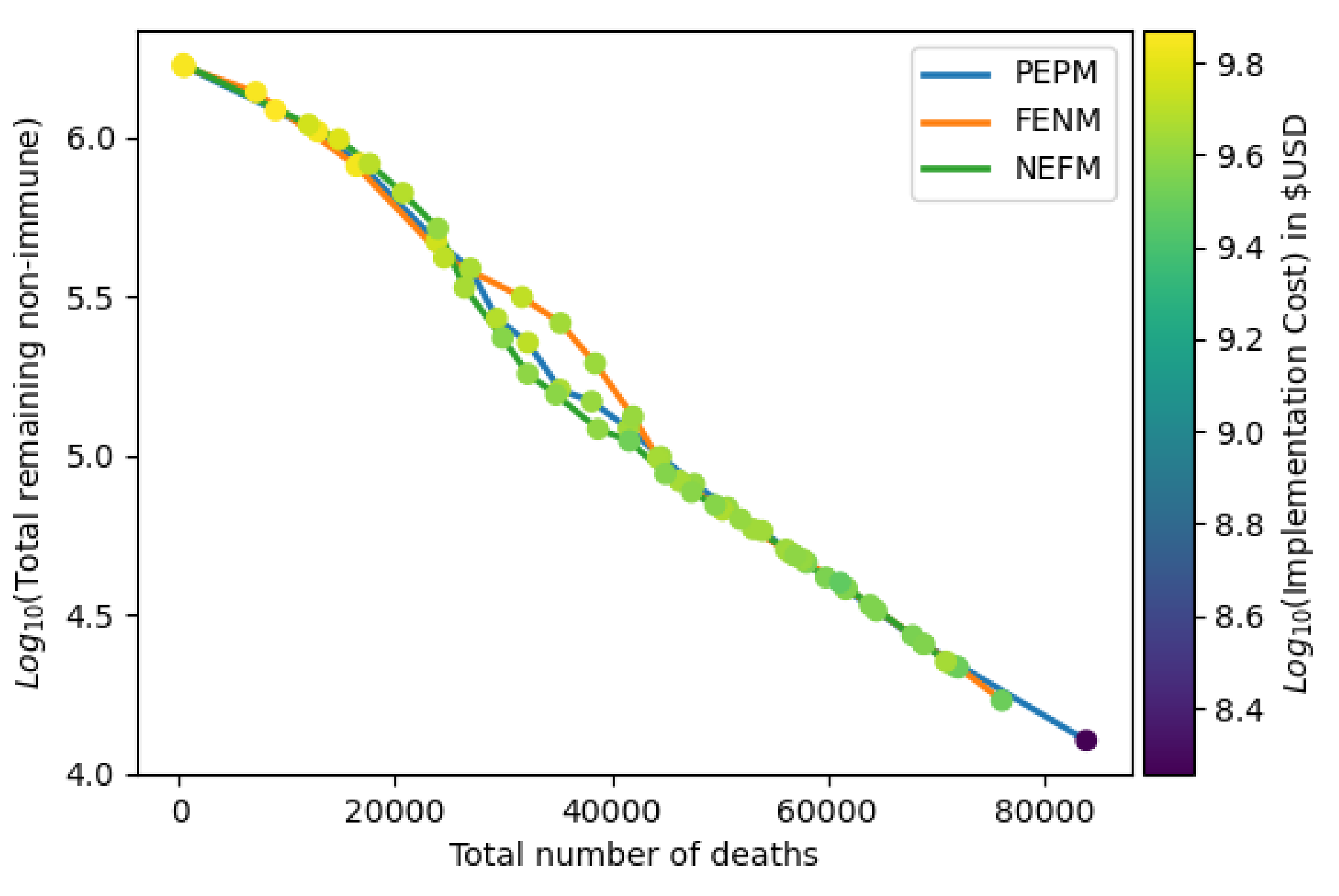
Figure 2 shows the Pareto curves for the trade-off between deaths and herd immunity found by the three different algorithms. The points on each curve were found by first setting a target number of deaths, and then finding the solution which meets the death target and has maximum herd immunity level (given by the number of recovered). The colors of the dots indicate the implementation costs of the solutions. In our case, the target death values ranged from 0 to 100,000 with steps of 4000. This graph can be used to assess various trade-offs between herd immunity level and number of deaths. For example, if fewer than 40,000 deaths is desired, the curve indicates that, under the best possible strategy, the number of remaining non-immune individuals in the population is roughly
. Alternatively, if, for example, the target is to reduce non-immune individuals below
, then this level is reached at the cost of about 60,000 deaths. The figure shows that the three algorithms produce similar trade-offs between deaths and herd immunity, but NEFM is slightly better in that the number of non-immune achieved for each death level is slightly smaller in most cases. This shows that NEFM solutions tend to give better trade-offs than the other two, indicating that an extended Monte Carlo algorithm is very effective in most cases in locating overall optima, even when no preliminary enumerative search is conducted.
Figure 3 shows the implementation costs of the Pareto optimal solutions shown in
Figure 2 as a function of death level. The dots’ colors measure the herd immunity level (indicated by the number of recovered). The figure shows that the NEFM algorithm is generally finding solutions with lower implementation cost, even while improving the herd immunity over the other two algorithms. This makes NEFM indisputably the best of the three algorithm variants, underscoring the key importance of Monte Carlo in the optimization process.
9.3. Temporal Characteristics of Pareto Optimal Solutions
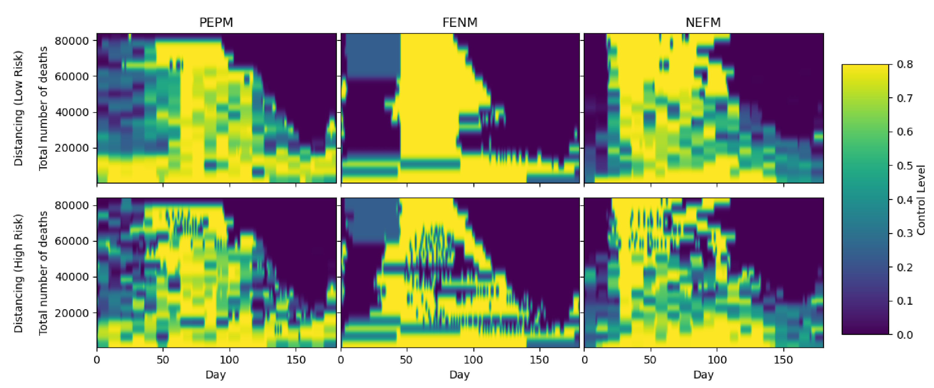
The heatmaps in
Figure 4 and
Figure 5 show the control measures (testing and distancing, respectively) that were implemented during the 180-day period for the different Pareto optimal solutions indicated in
Figure 2. The
x-axis shows the time in days, while the
y-axis represents the total number of deaths. The heatmap color for each pair of
values indicates the level for day
x of the controls applied for the Pareto optimal solution that results in a total of
y deaths over the 180-day period. Heatmap colors are associated with control levels according to the colorbar scale at right. For example, for PEPM, the low-risk testing control level on day 50 for a Pareto optimal strategy corresponding to 60,000 deaths, is around 0.7, as indicated by the yellow color of the pixel at the location
. On the other hand, for the same strategy on day 100, it is almost zero, as indicated by the dark blue color of the pixel a location
. To see the time progression of the Pareto optimal strategy that yields a total value of
d deaths, one may scan across the pixels at locations
for
.
Figure 4 shows low and high risk testing strategies for different death levels. By comparing across the three columns, it appears that PEPM is intermediate between FENM and NEFM. FENM consistently places heavy emphasis on testing for about the first quarter of the period (except for below about 15,000 deaths, as well as testing in the third quarter of the period for deaths between 20,000–40,000. PEPM also has early testing, but at a less intensive level and for a longer time (about the first third of the full period), and less late testing at a later time. NEFM shows spotty testing throughout the central part of the period, with much less emphasis especially at deaths above 50,000. Note that, for all three cases, for death levels above 40,000, there is a final day beyond which no testing is employed: for example, when deaths = 80,000, there is no testing after day 100. This indicates that the desired level of herd immunity has been reached, and no further control is necessary.
Comparing across the rows in
Figure 4, it appears that strategies applied to low-risk and high-risk subpopulations are similar, regardless of the algorithm. Consistently, testing applied to high-risk is slightly less intensive than for low risk. This may be due to the fact that, according to the contact matrix entries in (
3), low-risk individuals have at least three times as many daily contacts with both low- and high-risk persons. It follows that low-risk individuals play a much larger role in spreading the disease than high-risk individuals, so it is reasonable that testing should be more focused on them.
Figure 5 shows low and high risk distancing strategies for different death levels. Once again, PEPM is intermediate between FENM and NEFM. FENM has intensive distancing for the second quarter of the period, except below 20,000 deaths, where distancing stretches throughout the 180-day period. It appears that distancing levels are high during the intermediate period where testing is low, indicating a trade-off between the two control approaches. PEPM is similar, except there is also low-level distancing in the first quarter and intensive distancing is delayed. For NEFM, the period of intensive distancing is even longer, starting around 15–20 days and lasting for about half of the total period. Below 20,000 deaths, there is intensive distancing throughout the period for all three strategies, which explains why testing measures are greatly reduced for these death levels. It appears that distancing has a greater effect than testing in limiting disease exposure but is less preferred when some disease exposure is permitted in order to promote herd immunity.
As with testing, distancing strategies for low- and high-risk are similar regardless of death level for each of the three algorithms. Distancing also resembles testing in that above 40,000 deaths; there is a time at which all control is ceased, indicating that the disease has been sufficiently controlled and is left to run its course.
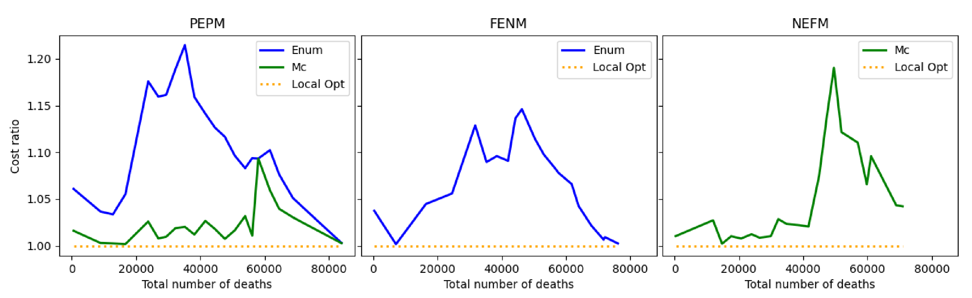
9.4. Relative Contributions of the Three Stages to the Overall Optimization
Figure 6 shows the contributions of the three optimization stages towards lowering the objective function in the overall solution process. The graphs compare the total cost obtained at the end of each optimization stage, in proportion to the final cost obtained by the completed optimization procedure. In the PEPM solution, the partial optimal enumerative solution produces a total cost that is generally between 5–25 percent higher than the final cost obtained by the three-stage algorithm, while the partial Monte Carlo stage improves this result to reach between 1–10 percent higher than the final solution. In the NEFM solution, the Monte Carlo stage reaches within 15 percent of the locally optimal solution. In the FENM solution, the enumerative alone reached within 15 percent of the final locally optimal solution.
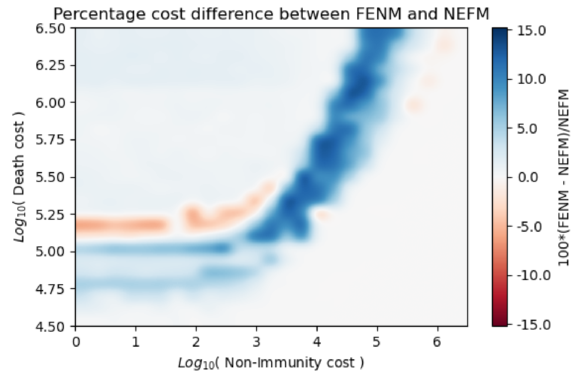
Figure 7 and
Figure 8 both show the percentage total cost difference between two different optimization methods produced by each combination of (non-immune cost, death cost). The base 10 logarithms of non-immune cost and death cost are plotted on the
x- and
y-axes, respectively. The heatmap color scale indicates the percentage cost difference between the optimized total costs obtained by the two different methods for each
combination.
Figure 7 shows that PEPM resulted in a higher total cost compared to NEFM for majority of the cost combinations, where cost differences range up to 15 percent. However, there is a region in the graph (non-immunity cost from
–
and death cost from
–
) where NEFM resulted in a higher cost than PEPM, with differences of up to about 5 percent. We will see in
Figure 9 that the Pareto solutions shown in
Figure 3 lie in the region where the difference between PEPM and NEFM is largest. The fact that NEFM outperforms PEPM for most cost combinations shows that the Monte Carlo stage has a larger effect on optimization than the enumerative method.
Figure 8 shows similar differences between FENM and NEFM. The fact that sometimes FENM and PEPM gives better results than NEFM shows that the enumerative method can be useful in providing the Monte Carlo stage with a suitable initial condition.
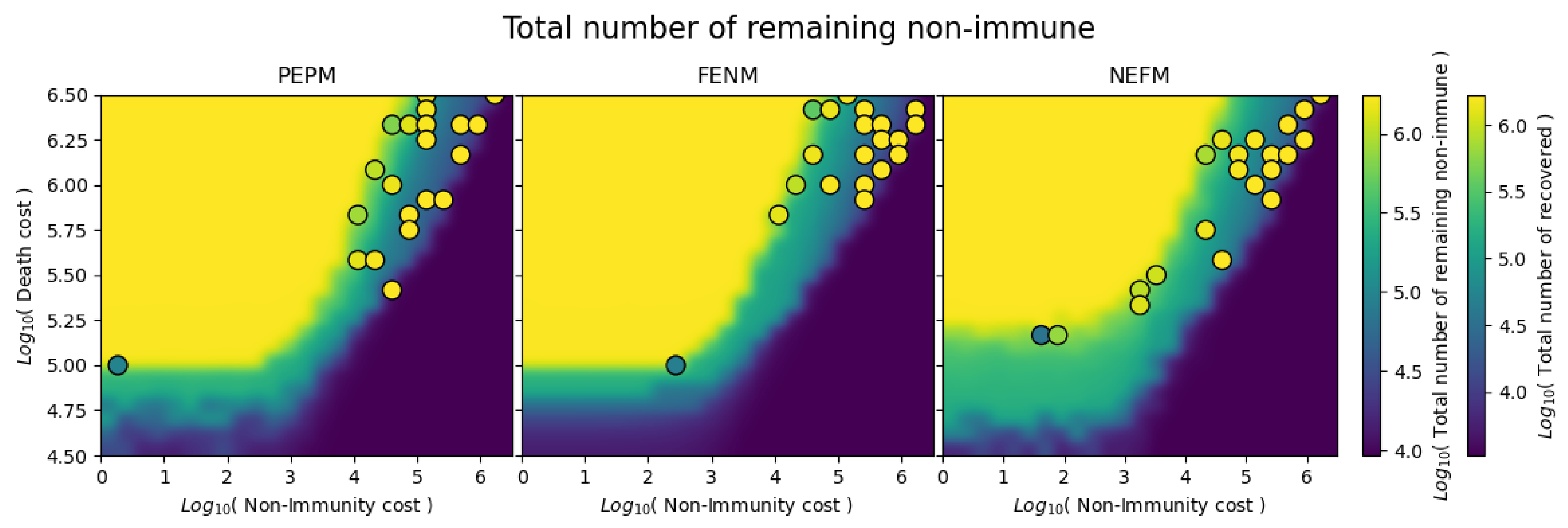
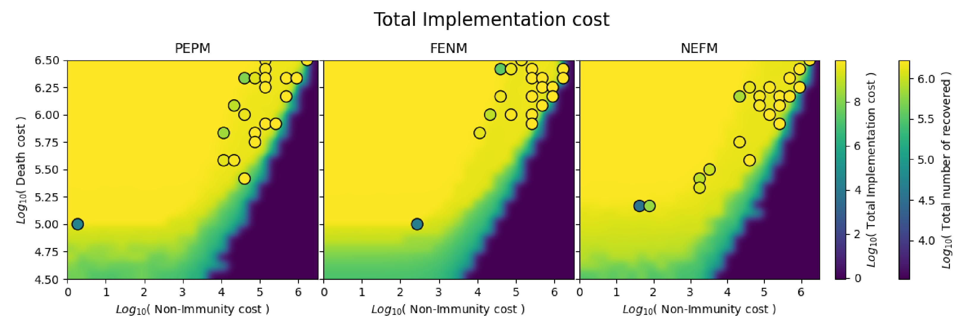
9.5. Death and Non-Immunity Cost Characteristics of Optimal Solutions
Figure 9,
Figure 10 and
Figure 11 show the locations of the Pareto optimal solutions shown in
Figure 3,
Figure 4,
Figure 5 and
Figure 6 within the same grid of non-immune and death costs that are shown in
Figure 7 and
Figure 8. The heatmap colors represent the quantity of interest for each graph, and the color scale for the heatmap is given by the first colorbar at right. The dots represent the (non-immune, death) cost combinations that correspond to the Pareto solutions shown in
Figure 3, and the second colorbar on the right interprets the colors of the dots, which correspond to the log base 10 of the final recovered population attained by the solutions represented by the dots.
Figure 9 shows a narrow transition region between cost combinations that produce few deaths (blue region) and those that produce many deaths (yellow region). The blue region corresponds to solutions that protect the population, but do not promote herd immunity, while the yellow regions show solutions where most of the population becomes immune. All of the Pareto optimal solutions are located in the transition region, for all three algorithms. By comparison with
Figure 7 and
Figure 8, it appears that most of the Pareto optimal solutions lie in the band where NEFM produces better optima than the other two algorithms.
Figure 10 is comparable to
Figure 9, except the heatmap shows the total number of remaining non-immune in the population after 180 days since the spread of the disease. This figure has similar characteristics to the previous figure—the low-death and high-death regions in
Figure 9 correspond to low and high levels of herd immunity, respectively. The only visible difference is the transition band between low and high herd immunity is wider and more clearly defined, especially for the FENM and PEPM algorithm variants.
Figure 11 is like the previous two figures except the heatmap shows the implementation cost. Low and high death regions correspond to high and low implementation costs, respectively. This figure differs from the previous two in that the transition band between high and low cost regions is somewhat lower, and the Pareto optimal solutions lie above the transition band instead of within. This is explained by the fact that our Pareto trade-off does not consider implementation cost, but is rather focused on deaths and herd immunity.
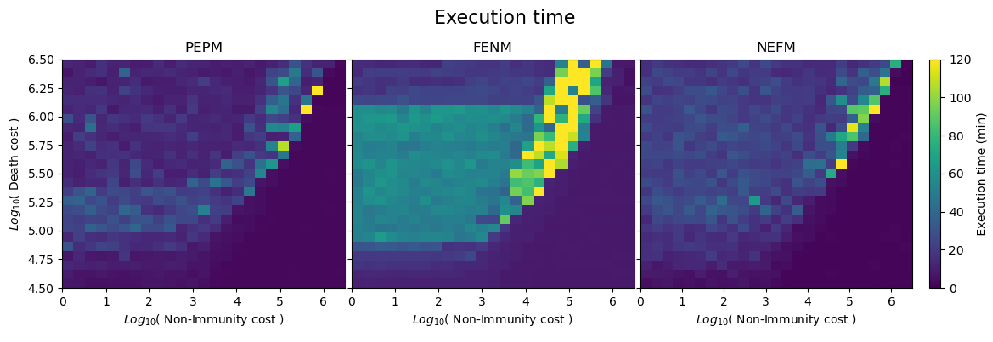
9.6. Execution Times for Three Algorithm Variants
The heatmaps in
Figure 12 display the runtimes obtained by the three different algorithms for the different (non-immune, death) cost combinations. All simulations were done on a Macbook Pro with a single 8-core 2.3 GHz Intel Core i9 processor and 16 GB RAM, running Python 3.7.7. In comparison with PEPM and NEFM, the FENM cost combination had the longest runtimes. The runtime for the cost combination (5.5, 3) on FENM was 80 min, while, on PEPM and NEFM, it was less than 40 min. This drastic change in the runtime can be explained by the expensive enumerative search that must compute a large number of solutions. It may also be noted that Pareto optimal solutions are among those that have longer runtimes.
Table 5 summarizes mean runtimes for the three optimization stages, for the three algorithm variants. The PEPM method had the shortest mean execution time, and NEFM was about 30% longer (recall, however, that NEFM obtained better solutions). FENM had by far the longest mean execution time, which was more than double that of NEFM.
10. Conclusions
This paper applies numerical methods for finding optimal controls to an SEIR epidemic model of COVID-19 in the city of Houston, TX, USA with low-risk and high-risk population groups. Available controls include COVID-19 testing and various distancing measures. We formulate an objective function that models the cost of COVID-19 by assigning monetary values to deaths and non-immunity, which can be adjusted to obtain solutions that meet different death or herd immunity level targets. We determine the local optimality conditions for the optimal control problem under testing and distancing controls.
A three-stage algorithm for numerically estimating optimal solutions is designed, and the performance (in terms of final solution total cost and computational cost) for three algorithm variants is thoroughly investigated. Of the three algorithm variants, the version that included the longest Monte Carlo stage without any enumerative solution gave the best control solutions, in terms of finding strategies that give better trade-offs between death and herd immunity and at lower cost. This implies that, of the three stages, the Monte Carlo stage has an especially significant effect on the optimization. However, results also show that all three stages contribute to the obtaining of good control solutions. Pareto optimal solutions that balance death versus herd immunity level exhibit a near-linear trade-off between these two variables, as shown in
Figure 2. The best obtained solutions show that distancing tends to outweigh testing, especially when the reduction of deaths is emphasized at the expense of herd immunity. Algorithm runtimes for the best-performing algorithm variant average under 20 min for a 180-day period, indicating that the algorithm is practically feasible for exploratory analysis.
Author Contributions
Conceptualization, L.V.T., V.M. and C.T.; methodology, L.V.T., V.M. and C.T.; software, L.V.T. and C.T.; validation, L.V.T. and C.T.; formal analysis, L.V.T., V.M. and C.T.; investigation, L.V.T. and C.T.; resources, L.V.T.; data curation, L.V.T.; writing—original draft preparation, L.V.T., V.M. and C.T.; writing—review and editing, L.V.T., V.M. and C.T.; visualization, L.V.T. and C.T.; supervision, C.T. and L.T.; project administration, L.T.; funding acquisition, L.T. All authors have read and agreed to the published version of the manuscript.
Funding
Researchers were supported by Texas A&M University-Central Texas (L.V.T.) and the German Academic Exchange Service (DAAD) (V.M.)
Data Availability Statement
Acknowledgments
The authors would like to thank the administration of the Institute of Mathematical and Physical Sciences (Porto- Novo, Benin) for facilitating the establishment of this research collaboration.
Conflicts of Interest
The authors declare no conflict of interest.
Abbreviations
The following abbreviations are used in this manuscript:
| COVID-19 | Corona virus disease 2019 |
| PEPM | Partial enumerative and partial Monte Carlo |
| FENM | Full enumerative and no Monte Carlo |
| NEFM | No enumerative and full Monte Carlo |
| N/A | Not applicable |
References
- Rao, A.V. A survey of numerical methods for optimal control. Adv. Astronaut. Sci. 2009, 135, 497–528. [Google Scholar]
- Supriatna, A.; Anggriani, N.; Nurulputri, L.; Wulantini, R.; Aldila, D. The optimal release strategy of Wolbachia infected mosquitoes to control dengue disease. Adv. Sci. Eng. Med. 2014, 6, 831–837. [Google Scholar] [CrossRef]
- Fischer, A.; Chudej, K.; Pesch, H.J. Optimal vaccination and control strategies against dengue. Math. Methods Appl. Sci. 2019, 42, 3496–3507. [Google Scholar] [CrossRef]
- Rodrigues, H.S.; Monteiro, M.T.T.; Torres, D.F. Dynamics of dengue epidemics when using optimal control. Math. Comput. Model. 2010, 52, 1667–1673. [Google Scholar] [CrossRef] [Green Version]
- Mbazumutima, V.; Thron, C.; Todjihounde, L. Enumerative numerical solution for optimal control using treatment and vaccination for an SIS epidemic model. BIOMATH 2019, 8, 1912137. [Google Scholar] [CrossRef] [Green Version]
- Haoxiang, Y.; Daniel, D.; Ozge, S.; David, P.M.; Remy, P.; Kelly, P.; Fox, J.S.; Meyers, L.A. Staged Strategy to Avoid Hospital Surge and Preventable Mortality, while Reducing the Economic Burden of Social Distancing Measures. Available online: https://sites.cns.utexas.edu/sites/default/files/cid/files/houston_strategy_to_avoid_surge.pdf?m=1592489259 (accessed on 27 January 2021).
- Ferguson, N.; Laydon, D.; Nedjati-Gilani, G.; Imai, N.; Ainslie, K.; Baguelin, M.; Bhatia, S.; Boonyasiri, A.; Cucunubá, Z.; Cuomo-Dannenburg, G.; et al. Report 9: Impact of non-pharmaceutical interventions (NPIs) to reduce COVID19 mortality and healthcare demand. Imp. Coll. Lond. 2020, 10, 491–497. [Google Scholar]
- Flaxman, S.; Mishra, S.; Gandy, A.; Unwin, H.J.T.; Mellan, T.A.; Coupland, H.; Whittaker, C.; Zhu, H.; Berah, T.; Eaton, J.W.; et al. Estimating the effects of non-pharmaceutical interventions on COVID-19 in Europe. Nature 2020, 584, 257–261. [Google Scholar] [CrossRef] [PubMed]
- Chang, S.L.; Harding, N.; Zachreson, C.; Cliff, O.M.; Prokopenko, M. Modelling transmission and control of the COVID-19 pandemic in Australia. Nat. Commun. 2020, 11, 5710. [Google Scholar] [CrossRef] [PubMed]
- Kucharski, A.J.; Russell, T.W.; Diamond, C.; Liu, Y.; Edmunds, J.; Funk, S.; Eggo, R.M.; Sun, F.; Jit, M.; Munday, J.D.; et al. Early dynamics of transmission and control of COVID-19: A mathematical modeling study. Lancet Infect. Dis. 2020, 20, 553–558. [Google Scholar] [CrossRef] [Green Version]
- Reddy, K.P.; Shebl, F.M.; Foote, J.H.; Harling, G.; Scott, J.A.; Panella, C.; Fitzmaurice, K.P.; Flanagan, C.; Hyle, E.P.; Neilan, A.M.; et al. Cost-effectiveness of public health strategies for COVID-19 epidemic control in South Africa: A microsimulation modeling study. Lancet Glob. Health 2021, 9, e120–e129. [Google Scholar] [CrossRef]
- Barbarossa, M.V.; Fuhrmann, J.; Meinke, J.H.; Krieg, S.; Varma, H.V.; Castelletti, N.; Lippert, T. A first study on the impact of current and future control measures on the spread of COVID-19 in Germany. medRxiv 2020. [Google Scholar] [CrossRef] [Green Version]
- Aldila, D.; Ndii, M.Z.; Samiadji, B.M. Optimal control on COVID-19 eradication program in Indonesia under the effect of community awareness. Math. Biosci. Eng. 2020, 17, 6355–6389. [Google Scholar] [CrossRef] [PubMed]
- Kantner, M.; Koprucki, T. Beyond just “flattening the curve”: Optimal control of epidemics with purely non-pharmaceutical interventions. J. Math. Ind. 2020, 10, 1–23. [Google Scholar] [CrossRef] [PubMed]
- Bouchnita, A.; Jebrane, A. A hybrid multi-scale model of COVID-19 transmission dynamics to assess the potential of non-pharmaceutical interventions. Chaos Solitons Fractals 2020, 138, 109941. [Google Scholar] [CrossRef] [PubMed]
- Lemecha Obsu, L.; Feyissa Balcha, S. Optimal control strategies for the transmission risk of COVID-19. J. Biol. Dyn. 2020, 14, 590–607. [Google Scholar] [CrossRef] [PubMed]
- Kouidere, A.; Khajji, B.; El Bhih, A.; Balatif, O.; Rachik, M. A mathematical modeling with optimal control strategy of transmission of COVID-19 pandemic virus. Commun. Math. Biol. Neurosci. 2020, 2020. [Google Scholar] [CrossRef]
- Thron, C.; Mbazumutima, V.; Tamayo, L.; Todjihounde, L. Cost Effective Reproduction Number Based Strategies for Reducing Deaths from COVID-19. J. Math. Ind. 2021. [Google Scholar] [CrossRef] [PubMed]
- Barker, A. Texas Medical Center Data Shows ICU, Ventilator Capacity vs. Usage during Coronavirus Outbreak. 2020. Available online: https://www.click2houston.com/health/2020/04/10/texas-medical-center-data-shows-icu-ventilator-capacity-vs-usage-during-coronavirus-outbreak/ (accessed on 27 January 2021).
- Lenhart, S.; Workman, J.T. Optimal Control Applied to Biological Models; CRC Press: Boca Raton, FL, USA, 2007. [Google Scholar]
- Pontryagin, L.S. Mathematical Theory of Optimal Processes; Routledge: London, UK, 2018. [Google Scholar]
- Chiang, A.C. Elements of Dynamic Optimization; McGraw-Hill: New York, NY, USA, 1992. [Google Scholar]
- Kamien, M.I.; Schwartz, N.L. Sufficient conditions in optimal control theory. J. Econ. Theory 1971, 3, 207–214. [Google Scholar] [CrossRef]
- Mangasarian, O.L. Sufficient conditions for the optimal control of nonlinear systems. SIAM J. Control. 1966, 4, 139–152. [Google Scholar] [CrossRef]
Figure 1.
Multicompartment structure of COVID-19 transmission model (taken from [
6]).
Figure 1.
Multicompartment structure of COVID-19 transmission model (taken from [
6]).
Figure 2.
Pareto curves showing the trade-off between total deaths and final herd immunity level, for the three different algorithm variants. Solutions are given by colored dots, where dot colors indicate the solution implementation cost according to the color scale at right.
Figure 2.
Pareto curves showing the trade-off between total deaths and final herd immunity level, for the three different algorithm variants. Solutions are given by colored dots, where dot colors indicate the solution implementation cost according to the color scale at right.
Figure 3.
Implementation costs for the Pareto optimal solutions shown in
Figure 2 at different death levels, for the three different algorithm variants. Solutions are given by colored dots, where dot colors indicate the number of recovered individuals according to the color scale at right.
Figure 3.
Implementation costs for the Pareto optimal solutions shown in
Figure 2 at different death levels, for the three different algorithm variants. Solutions are given by colored dots, where dot colors indicate the number of recovered individuals according to the color scale at right.
Figure 4.
Testing control measures corresponding to the Pareto-optimal solutions in
Figure 2. The first row of figures shows the daily progression of low-risk testing control levels for PEPM, FENM, and NEFM for Pareto optimal strategies that attain different overall deaths, as indicated on the
y-axis of the graphs. The second row shows corresponding figures for high-risk control levels for the PEPM, FENM, and NEFM solutions.
Figure 5.
Social distance control measures corresponding to the Pareto-optimal solutions in
Figure 2. The first row of figures shows the daily progression of low-risk distancing control levels for PEPM, FENM, and NEFM for Pareto optimal strategies that attain different overall deaths, as indicated on the
y-axis of the graphs. The second row shows corresponding figures for high-risk distancing levels for the PEPM, FENM, and NEFM solutions.
Figure 6.
Ratio of costs achieved following different optimization stages compared to the final cost obtained following local optimization. Costs are given as a function of the number of deaths in the Pareto-optimal calculated solution.
Figure 6.
Ratio of costs achieved following different optimization stages compared to the final cost obtained following local optimization. Costs are given as a function of the number of deaths in the Pareto-optimal calculated solution.
Figure 7.
Heatmap showing percentage difference in total cost between final solutions obtained by PEPM and NEFM, as a function of death and non-immunity cost.
Figure 7.
Heatmap showing percentage difference in total cost between final solutions obtained by PEPM and NEFM, as a function of death and non-immunity cost.
Figure 8.
Heatmap showing percentage difference in total cost between final solutions obtained by FENM and NEFM, as a function of death and non-immunity cost.
Figure 8.
Heatmap showing percentage difference in total cost between final solutions obtained by FENM and NEFM, as a function of death and non-immunity cost.
Figure 9.
Heatmap showing number of deaths as a function of death and non-immunity costs under PEPM, FENM, and NEFM algorithms, respectively. Pareto optimal solutions are indicated by hollow dots, and the dot colors correspond to number of recovered according to the color scale at the far left. The figure shows that all Pareto optimal solutions occur in the transition region between death-nonimmune cost combinations producing few deaths (blue region) and those corresponding to many deaths (yellow region).
Figure 10.
Heatmap showing remaining non-immune individuals as a function of death and non-immunity costs under PEPM, FENM, and NEFM algorithms, respectively. Pareto optimal solutions are indicated by hollow dots, and the dot colors correspond to the number of recovered according to the color scale at the far left. The figure shows that all Pareto optimal solutions occur in the transition region between death-nonimmune cost combinations producing low herd immunity (blue region) and those corresponding to high herd immunity (yellow region).
Figure 11.
Heatmap showing total implementation cost as a function of death and non-immunity costs under PEPM, FENM, and NEFM algorithms, respectively. Pareto optimal solutions are indicated by hollow dots, and the dot colors correspond to number of recovered according to the color scale at the far left.
Figure 12.
Runtimes of PEPM, FENM, and NEFM algorithms as a function of death and non-immunity non-immunity costs.
Figure 12.
Runtimes of PEPM, FENM, and NEFM algorithms as a function of death and non-immunity non-immunity costs.
Table 1.
Baseline parameters used in the model [
6].
Table 1.
Baseline parameters used in the model [
6].
| Parameters | Interpretation | Values |
|---|
| baseline transmission rate | 0.0640 |
| recovery rate on asymptomatic compartment | Equal to |
| recovery rate on symptomatic non-treated
compartment | |
| symptomatic proportion | |
| exposed rate | |
| pre-asymptomatic rate | Equal to |
| pre-asymptomatic rate | |
| P | proportion of pre-symptomatic transmission | |
| relative infectiousness of symptomatic individuals | |
| relative infectiousness of pre-symptomatic individuals | |
| relative infectiousness of infectious individuals in
compartment | |
| infected fatality ratio, age specific (%) | |
| symptomatic fatality ratio, age specific (%) | |
| recovery rate in hospitalized compartment | |
| Symptomatic case hospitalization rate % | |
| rate of symptomatic individuals go to hospital, age-specific | |
| rate from symptom onset to hospitalized | |
| rate at which terminal patients die | |
| hospitalized fatality ratio, age specific (%) | |
| death rate on hospitalized individuals, age specific | |
| Hospitals’ capacity to treat seriously ill patients | 3000 [19] |
| number of deaths from the people who are put on respirators | 1/3 |
Table 2.
Cost coefficients and level parameters used in simulation.
Table 2.
Cost coefficients and level parameters used in simulation.
| Parameters | Interpretation | Values |
|---|
| minimum testing cost per person | $0 |
| linear testing cost coefficient | $2.3/person/day |
| quadratic rate of increase of per capita testing cost | $27/person/day |
| constant per capita social distancing costs | $0 |
| quadratic rate of increase of per capita social distancing cost | $40/person/day |
| cost per death | – (assumed) |
| cost multiplier for remaining infected | 2 (assumed) |
| cost per remaining non-immune | – (assumed) |
| maximum testing control level | |
| maximum social distancing control level | |
Table 3.
Parameters for Monte Carlo algorithm.
Table 3.
Parameters for Monte Carlo algorithm.
| Symbol | Value | Description |
|---|
| 20 | Number constant intervals for controls |
| 10 | Maximum number of non-improving objective cost iterations |
| 5 | Maximum number of non-improving cooling cycles |
| 0.95 | Memory factor used in computing the mean increase |
| 0.95 | Temperature multiplier (scale factor) |
| 0.95 | Increment in during cooling |
| 4 | Unscaled temperature at start of new cooling cycle |
| 0.5 | P matrix adjustment |
| 0.5 | U matrix adjustment |
| 0.5 | R matrix adjustment |
| 0.1 | Initial magnitude of control perturbations |
Table 4.
Parameters for each of the three optimization methods.
Table 4.
Parameters for each of the three optimization methods.
| | Algorithm Combinations |
|---|
| Optimization Stage | PEPM | FENM | NEFM |
|---|
| Enumerative | Intervals = 3 | Intervals = 4 | N/A |
| Monte Carlo |
| N/A |
|
Table 5.
Average execution time for each method.
Table 5.
Average execution time for each method.
| | Execution Time |
|---|
| Simulation | Enumerative | Monte Carlo | Local Optimization | Total |
|---|
| PEPM | 1.03 min | 1.23 min | 11.79 min | 14.05 min |
| FENM | 6.85 min | 0.00 min | 31.48 min | 38.33 min |
| NEFM | 0.00 min | 5.39 min | 12.53 min | 17.92 min |
| Publisher’s Note: MDPI stays neutral with regard to jurisdictional claims in published maps and institutional affiliations. |
© 2021 by the authors. Licensee MDPI, Basel, Switzerland. This article is an open access article distributed under the terms and conditions of the Creative Commons Attribution (CC BY) license (https://creativecommons.org/licenses/by/4.0/).


