
Stable Topological Summaries for Analyzing the Organization of Cells in a Packed Tissue


Departamento de Matemática Aplicada I, E.T.S. Ingeniería Informática, Universidad de Sevilla, Av. Reina Mercedes S.N., 41012 Sevilla, Spain
*
Author to whom correspondence should be addressed.
†
These authors contributed equally to this work and are listed in alphabetical order.
Mathematics 2021, 9(15), 1723; https://doi.org/10.3390/math9151723
Submission received: 18 May 2021
/
Revised: 17 July 2021
/
Accepted: 17 July 2021
/
Published: 22 July 2021
(This article belongs to the Special Issue Computational Algebraic Topology and Neural Networks in Computer Vision)
Abstract
:We use topological data analysis tools for studying the inner organization of cells in segmented images of epithelial tissues. More specifically, for each segmented image, we compute different persistence barcodes, which codify the lifetime of homology classes (persistent homology) along different filtrations (increasing nested sequences of simplicial complexes) that are built from the regions representing the cells in the tissue. We use a complete and well-grounded set of numerical variables over those persistence barcodes, also known as topological summaries. A novel combination of normalization methods for both the set of input segmented images and the produced barcodes allows for the proven stability results for those variables with respect to small changes in the input, as well as invariance to image scale. Our study provides new insights to this problem, such as a possible novel indicator for the development of the drosophila wing disc tissue or the importance of centroids’ distribution to differentiate some tissues from their CVT-path counterpart (a mathematical model of epithelia based on Voronoi diagrams). We also show how the use of topological summaries may improve the classification accuracy of epithelial images using a Random Forest algorithm.
1. Introduction
Epithelia morphogenesis is key to understanding the development of tissues and organs. The complete picture of how epithelial tissues change or maintain their inner organization is still unknown. In particular, it is known that diseases and mutations might affect the usual arrangement of cells in epithlelial tissues [1,2,3]. Looking for methods that can quantify the arrangement of cells is still an open and interesting problem [4]. These tissues are formed by tightly assembled cells, with almost no intercellular spaces. The apical surfaces of tissues formed by columnar epithelial cells are similar to convex polygons [1] and form natural tessellations. This allows for the identification of each cell with a polygon with as many sides as neighboring cells. The study of epithelial organization has been mainly focused on the polygon distributions [1], that is, the distribution of the number of neighbors (sides) of the cells (polygons). In [5], the authors looked for differences in the polygon distribution of two proliferative stages of drosophila wing disc. In later studies, the concept of centroidal Voronoi tessellation (CVT) was used, which is a Voronoi diagram where the point generating each region coincides with its centroid. The Lloyd algorithm is an iterative algorithm that, starting from a random cloud of points, produces a series of Voronoi diagrams, that we will denote by (, that converge to a CVT [6]. Such a sequence of Voronoi diagrams is called a CVT-path in [7]. In that study, the authors compared the polygon distributions of images of natural packed tissues with those of the CVT-path and showed that the former fit to the polygon distribution of specific Voronoi diagrams inside the CVT-path. A different approach was developed in [4], where the authors provided an image analysis tool implemented in the open-access platform FIJI, to quantify epithelial organization based in computational geometry and graph theory concepts. More specifically, considering the contact graph, that is, the graph generated by the cells (vertices) and the cell-to-cell contacts (edges), they searched locally for specific motifs represented by small subgraphs (graphlets) to characterize the tissue.
The previous approaches have two main problems: assuming that the cells are similar to convex polygons and that the analysis is mostly related to local features, ignoring other aspects of the contact graph, such as, for example, what types of polygons are connected among them.
As pointed out by Villoutreix in his thesis, the standard topological analysis of complex networks is very limited in this context, since all contact graphs are planar (see [8], Section 8.2.2). In particular, techniques such as topological indices, which perform well in other contexts [9], are not expected to be useful in packed tissues. In [8], the author proposed the use of topological data analysis (TDA) as a possible solution to obtain richer information than just the polygon distribution.
In addition, it has also been proven that any realistic model of epithelial tissues must consider spatial correlation between cells [10], and neither the polygon distribution, nor the contact network, nor the graphlets analysis take it into consideration. In this paper, we will formalize the intuitive notion of inner organization of the tissue using its contact graph and its spatial centroid distribution. In addition, we will show that TDA may work when cells are not convex-like. Finally, we add TDA variables to a machine learning workflow to improve the classification of images coming from cellular tissues. We also explain some interpretations of the TDA variables at the tissue level, providing new insights about the organization of the cell.
1.1. Previous Topological Data Analysis Approaches
Recall that topology is the branch of mathematics that deals with properties of space that remain invariant under continuous transformations. These properties may be extremely important when the space is a network.
Nowadays, TDA is spreading as a useful approach in very different scientific fields, playing an increasing role in biological and, in general, biomedical imaging. Its main analysis tool, persistent homology [11,12], has been successfully applied in solving problems such as tumor segmentation [13], analyzing biological networks [14], monitoring the evolution of glioblastoma [15], and to improve the diagnostics of chronic obstructive pulmonary disease [16]. Persistent homology studies the evolution of homology classes and their lifetimes (persistence) in an increasing nested sequence of spaces (called a filtration). A filtration could be thought of as a multi-scale combinatorial model that represents topological (and somehow, geometric) information of the data. All the information obtained by persistent homology can be codified as a combinatorial invariant, called persistence barcode, which acts as a topological signature of the filtration, and therefore of the original dataset.
In [8], a model for analyzing the contact graph of the cell tissues using sub and sup filtrations (see Section 2.3.1) was presented. To our knowledge, this was the first experiment relating epithelial tissues with TDA. Its nature was exploratory and the results were similar to the ones obtained using the mean and variance of the degree of the cells. Another problem of this analysis was that the polynomial variables used for analyzing the barcodes were not stable with respect to the bottleneck distance (see Section 2.5). Defining stable polynomial variables was one of the main reasons why tropical coordinates were defined in [17]. We have found the work in [8] extremely useful as a first approach, and this paper can be seen, partially, as a continuation of it. Independently, a similar approach was presented in the conference paper [18]. In this case, persistent entropy was used instead of polynomial variables. Again, stability was not guaranteed, since the number of bars of each barcode was not fixed, as required in [19] for a stable result. Finally, another approach was introduced in the conference paper [20]. In that case, instead of using the contact graph of the cells, spatial distribution of their centroids was studied, using the alpha filtration (or alpha-complex), which was constructed over the Delaunay complex generated by the set of centroids [21]. Nevertheless, keeping the infinity bar in the barcodes, as in [20], made the summaries depend on the original scale of the image, introducing bias in the analysis. One of the major motivations of this paper was to solve that problem. Needless to say that finding a setting for normalizing the barcodes (so that they can be compared), while guaranteeing the stability of the variables used to analyze them, is far away from being trivial and requires a mathematical analysis even for a specific case study such as this one.
This paper can be seen as a continuation of the conference papers [18,20], where the experiments have been extended and improved, adding more variables and combining different filtrations. In addition, an exhaustive theoretical analysis is presented to avoid the bias present in those preliminary studies.
Recently, two papers applying persistent homology to cell images have been published. In [22], the authors use cycles to analyze the clustering of epithelial cells as self-propelled particles (not forming packed tissues). In [23], persistent homology is used to characterize the spatial arrangement of immune and epithelial (tumor) cells within the breast cancer immune microenvironment. In this case, pixel stain intensity is used as a filter function.
1.2. Overview of the Paper
In Section 2, we will modify the methods appearing in [8,20] to guarantee the stability in the entire procedure. Mathematical proofs to support correctness are provided. No assumption about convexity of the cells is needed. In Section 3, a rigorous statistical analysis of the results for tissues (both epithelium and CVTs) is carried out using TDA variables. Additionally, these variables will be used to improve the performance of a Random Forest classification of the tissues based on their neighbors’ distribution. Interpretations of some of the variables at the tissue level are provided. Finally, we will summarize the results in Section 4 and propose new interesting questions arising from this paper that might be of interest for different fields, such as developmental biology, pattern recognition or TDA.
2. Materials and Methods
Our aim is to assign to each epithelial image an invariant, called a persistence barcode, representing inner topological and geometrical information. We would like to analyze these persistence barcodes using numerical variables. There are three main difficulties:
- Finding a correct data normalization which does not include bias in our analysis due to the number of cells or the scale of the image.
- Guaranteeing that our variables only measure topological-geometrical properties. In particular, they should be invariant to rotation or scale changes.
- Proving robustness of our variables with respect to the cell organization.
2.1. Input Data
Our method is suitable for the topological analysis of the organization of segmented regions that partition a portion of plane. In this paper, the images for our experiments come from several types of (real) epithelial tissues as well as different mathematical tessellations. The segmented images of epithelial tissues considered are available as supplementary material in the article [24]. More specifically, there are epithelial images taken from model organisms traditionally used in developmental biology, such as images from chicken tissues: chicken embryonic ectoderm (cEE) images, chicken neural tube (cNT) images, and images from Drosophila tissues: Drosophila notum prepupa (dNP) images, wing disc in the larva (dWL) and prepupal (dWP) stages of development. The tissues dWL and dWP are taken from two proliferative stages separated by only 24 h of development and are considered to be particularly difficult to distinguish between. Further information about the way these images were obtained and segmented can be found in [24].
The morphology of cells in some epithelial tissues is commonly approximated by Voronoi tessellations [25], however we also consider the so-called CVT-path: a sequence of Voronoi diagrams which converges to a Central Voronoi Distribution (a Voronoi diagram whose centroids are also its seeds). Information of how the CVT-path is generated can be found in [7]. More specifically, is the Voronoi diagram of a point cloud following a Poisson distribution. is obtained from inductively following the Lloyd algorithm [26]:
- Compute the centroids of the regions in the Voronoi Diagram .
- Set these centroids as the new seeds and generate the Voronoi diagram .
In order to obtain information from the regions such as the centroids, the Matlab function regionprops was used. For the contact graph, a small dilation was performed on each region and labels of adjacent regions reached by the dilation were retrieved. Cells are said to be valid if they do not touch the exterior limits of the image. Only valid cells will be processed. The data extraction procedure, together with the whole code, can be found in a publicly available repository (github.com/Cimagroup/topo-summaries-for-packed-tissues (accessed on 18 May 2021)).
2.2. Normalization and Cell Selection
In order to avoid the bias induced by the number of valid cells in each tissue, we will always consider the same number of cells from each image to proceed to the topological analysis. Besides, this normalization is key to prove some stability results in Section 2.6 and Section 2.7. Although a higher number of cells is, in general, better to have a more global picture of the organization, the amount considered will be constrained by the minimum number of cells in the images of the given database. The number of valid cells in the whole set of images ranges from 140 to 1102, see Table 1. Then, as a starting point, we can fix as the number of cells picked. Unfortunately, a rare event happens in the first cEE image: some valid cells are completely surrounded by non-valid cells, making them disconnected from the rest. We have decided to dismiss it as an outlier (representing of the total sample). Then, we will fix , as it is the second minimum number of cells appearing in Table 1. We follow Algorithm 1 [20] to select the desired number of cells in each image. In Figure 1, an intuitive idea of how the algorithm works is provided. From now on, we will denote as valid cells only those selected by this algorithm.
| Algorithm 1 Spiral selection of regions |
|
2.3. Simplicial Complexes and Filtrations
A k-simplex (or simplex of dimension k) in is the convex hull of a set of affinely independent points . The points of are called the vertices of and the subsets of form the faces of . That is, each ℓ-simplex contained in with is called a face of . A (geometric) simplicial complex is formed by a set of simplices satisfying:
- Every face of a simplex in is also in .
- The intersection of any two simplices in is either a face of both simplices or the empty set.
The dimension of a simplicial complex is the maximum of the dimensions of its simplices. The combinatorial description of as finite subsets of the whole set of vertices V (without considering the geometric embedding in ) is known as an abstract simplicial complex. In the following, when we refer to a simplicial complex, we mean an abstract simplicial complex.
A filtration over a simplicial complex is a finite nested sequence of simp- licial subcomplexes:
It is commonly defined using a monotonic function , i.e., for any two simplices , if is a face of , then . That way, if are the function values of all the simplices in , then the subcomplexes , for define a filtration over . We may call f a filtration when we actually refer to the filtration induced by f.
We will use three types of filtrations: the clique complex filtration sub, the clique complex filtration sup, and the Vietoris-Rips filtration rips.
2.3.1. The Sub and Sup Filtrations
Since we know which valid cells are neighbors of each other, we can build a graph representing this relation as edges. We denote it as a contact graph. We construct the clique complex of a graph, , adding a k-simplex whenever the graph has a clique formed by the vertices . Define the sub, sup filtration [8] over the clique complex of a contact graph using the following functions,
where is the degree of the vertex x (i.e., number of valid neighbors of the cell representing x) and a simplex of the simplicial complex. We use the value 15 in the sup filtration since it is rare to find a cell with such a number of neighbors, and in fact, there is not such a cell in our samples. Note that both sup and sub only carry information about the topology of the contact graph of the cells (it is a topological invariant). See Figure 2 for two examples.
2.3.2. The Rips Filtration
Another strategy is to obtain the centroid of each cell and study their distribution. In order to do that, we will use the Vietoris-Rips filtration [21]. It is constructed using the function:
over the simplex generated from the whole set of centroids. See Figure 3 for an example. It is important to emphasize that the immersion of the point cloud of the image to depends on the “distance per pixel relation” of the original image, and so does rips. Then, rips is not scale-invariant. We would like to eliminate this bias with a normalization process, but due to stability arguments, we will apply it in the next step and not directly on the filtration.
2.4. Persistent Homology and Barcodes
Intuitively, homology formalizes the notion of m-dimensional holes. A 0-dimensional hole is a connected component, a 1-dimensional hole is a tunnel (or a cycle in a graph), a 2-dimensional hole is a cavity, and so on. More specifically, homology provides a procedure to assign to a simplicial complex , a vector space as follows:
First, define the m-chains of , , as the vector space over a field , with the basis being the set of m-dimensional simplices of . In this paper, we will use . If is an m-simplex, define the boundary operator in each m-simplex as , where F are the faces of . Then, extend it linearly to obtain . The m-th homology, , is the vector space:
where ker is the kernel of ∂ and im is the image. Each of the classes of can be seen as a hole of . The m-betti number, , is interpreted as its amount of m-dimensional holes.
Besides, if we have two simplicial complexes, , homology induces a linear map between and . In this case, can be seen as the number of m-dimensional holes shared by both simplicial complexes.
Persistent homology studies how the m-dimensional holes appear and disappear in a filtration . Fix a pair of numbers and . Following the previous reasoning, note that the value:
can be interpreted as the number of d-dimensional holes which appear at i and disappear at j. Note that and are values out of the original filtration. In order to proceed with the calculation, we can set them as 0. Since does not correspond to a simplicial complex; actually, holes which disappear at may be considered to persist up to infinity instead. This information is summarized in the m-dimensional barcode (or m-barcode), a multi-set of intervals:
where each interval appears times (its multiplicity). Nevertheless, we want to use sets instead of multi-sets, so a barcode, B, will be described as a set of intervals, each appearing repeated as many times as its multiplicity,
We provide an example in Figure 4. Further details on homology and persistent homology can be found in [21].
2.5. Bottleneck Distance and Stability
One of the main advantages of persistent homology with respect to classical homology, is that it is stable regarding small modifications of the input. In order to introduce this result, we need a notion of closeness for persistence barcodes.
Similarities between persistence barcodes can be measured by bottleneck distance. A -partial matching between barcodes is a collection of pairs , such that:
- For each , there is at most one , such that and vice versa.
- If , then .
- If (or in ) is unpaired, then .
The bottleneck distance between two barcodes is defined as:
The following stability result can be found in [21]. Given two filtrations , we have:
In our case, cell tissues with similar contact network or similar centroid distribution provide similar barcodes.
2.6. Barcodes’ Normalization
Barcodes are not good for statistical analysis, as shown in [27]. We will use numerical variables calculated from the barcodes, but we need to deal with infinity bars beforehand. Consider a barcode B representing a sub or sup filtration. We would like to somehow keep infinity bars since they provide information about the barcode. Define the function , which gives the same barcode but with infinity bars transformed to . In [19], it was shown that:
In our sample, no cell has 15 or more neighbors, so fixing will map infinity bars to bars that are always longer than the others. Note that sub and sup barcodes are always in the same units (number of neighbors) and can be compared between them. In addition, they are invariant to rotations and scale of the input, by definition.
In the rips case, the last complex appearing in the filtration is always contractible, so there are not infinity bars with dimensions greater than 0, and only one infinity interval, , in the 0 dimensional persistent homology. Then, infinity bars do not provide information in this context so we eliminate them using . Note that this is equivalent to calculating the reduced homology.
Recall that we mentioned in Section 2.3.2 that the centroids from which rips is defined still carry the units from the image, and so does the barcode associated to rips. Hence, it is not invariant to scale, since it depends on the distance matrix of the point cloud. The following normalization solves this problem: we are dividing each barcode by the sum of the lengths of the bars. More specifically, given with no infinity bars, define and . It is a direct consequence from ([19], lemma 3.9) that:
where is the maximum number of bars between and . Note that for any barcode B coming from the 0-dimenional rips, we have number of bars (one for each of the n cells minus the infinity bar) and , where is the average length of the bars. Then, for all 0-dimensional rips barcodes coming from our experiment:
where is the minimum of all averages, . Note that cannot be arbitrarily small since there are physical constraints for the size of cells in the tissue. Unfortunately, the 1-dimensional case is not stable under this normalization since we cannot find a lower bound for L. We drop the 1-dimensional rips barcodes from the experiment. As the following result shows, this normalization makes rips barcodes scale-invariant.
Proposition 1.
Fix a normed vector space and the induced distance, d. Fix a scalar, α, and consider two point clouds, and . Let and be their barcodes coming from rips. Then, .
Proof.
Note that for any two points:
Then, if the induced filtration by is f, the one from is . In particular, in the first case must be equal to in the second case. This means that barcodes are also proportional, and , so:
□
In particular, it works in our setting since with the Euclidean distance is a normed vector space. Then, from each image, we have five barcodes, four coming from 0- and 1-dimensional sub and sup filtrations and coming from 0-dimensional rips. From now on, when we mention a barcode coming from any of these filtrations, we assume the corresponding has already been applied.
2.7. Stable Topological Summaries
In the previous section, we saw that barcodes with the bottleneck distance are stable with respect to modifications in the input. Then, variables defined on the barcodes which are stable with respect to the bottleneck distance will be stable with respect to the input as well.
In this section, we will describe the variables used in this paper and study their stability.
2.7.1. Persistent Entropy
Persistent entropy [28,29] is a topological summary that can be seen as an adaptation of Shannon entropy (Shannon index in ecology) to the persistent homology context. Given a barcode with finite bars , consider the length of the bars and their sum . Then, its persistent entropy is:
when computed over an m-dimensional barcode B. The stability result appearing in [19] is simplified greatly in our case. In particular, we have that the 0-barcodes coming from rips satisfy after normalization.
First, recall a result relative to the Shannon entropy, .
Proposition 2
([30], p. 664). Let P and Q be two finite probability distributions (seen as vectors in ), and let and be, respectively, their Shannon entropy. If , then:
We can transform the previous proposition in the following result for persistent entropy:
Proposition 3.
Let A and B be two barcodes with the same number of bars, n, all of them starting at 0 and satisfying . If , then:
Proof.
Note that since both barcodes have the same number of bars and all of them start at 0, the matching provided by the bottleneck distance is a one-to-one mapping between both sets of intervals. Then, we can order the barcodes in such a way that the bars matched by bottleneck distance are listed in the same position. Besides, since we have , we can treat its barcode as a finite probability distribution . Name Q the probability distribution of B. Note that . Then, substituting in the formula in Proposition 2 and using , the result follows. □
Then, this proposition provides a stability result for the rips filtration. In the sub and sup case, the result is not straightforward, but we can still talk about stability (see Theorem 3.12 in [19]). Henceforth, we will refer to the persistent entropy of a d-dimensional barcode as .
2.7.2. Tropical Polynomials
Tropical coordinates allow for the definition of stable polynomials over barcodes, as explained in [17]. These polynomials are defined on the max-plus semi-ring , with addition and multiplication being defined as:
In particular, for the variables , polynomials of this semi-ring are written (with the usual notation) as:
where and . If we make an analogous definition for barcodes, using the length of the bars, , as variables, we obtain polynomials of the form:
These types of polynomials are shown to be stable with respect to the bottleneck distance.
Proposition 4
([17]). Let F be a polynomial defined over barcodes , as stated before. Then, there exists a constant C, such that:
2.7.3. Persistence Landscapes
A persistence landscape [31] is a sequence of summary functions obtained from a barcode. Given a barcode , perform the change of coordinates:
The rescaled rank function, is defined as:
The persistence landscape is the set of functions with given by:
Persistence landscapes are related with tropical polynomials. In particular, they are an example of what is called tropical rational function (see [17,32]). See Figure 5 for an illustration. There is also a stability result available, as follows:
Proposition 5
Since we are interested in variables and not summary functions, we will use the 1-norm of . Note that for sub and sup, the domain of the landscape is restricted to , and for rips, all the intervals will lie in . Then, in our case:
where or 1 depending on the filtration.
We have seen how to obtain numerical summaries from the tissue images, each of them stable with respect to the filtration induced by the cell organization. This means that, if their contact network or their centroid distribution are similar (up to scaling), the resulting variables will be similar. We have proved that these summaries satisfy the desired conditions: they measure topological and geometrical properties (at least up to scaling or rotation), they are robust to modification in the organization of the cells (we mean with respect to modification in their contact network or centroid distribution), and all barcodes have been normalized to avoid bias when comparing them.
3. Results
Our experiment is divided into two parts. First, we analyze the barcodes using statistical techniques. Then, we try to classify the images using Random Forests. In both cases, we use variables coming from the previous section. We selected different polynomials and k values for the landscapes. The notation is as follows: means the summary corresponding to the norm of the landscape computed from the d-dimensional persistence barcode of the filtration filt with parameter k. Instead of a fixed number, we may express k as a percentage together with the letter N. For example, means we have used the sub filtration and . For , we have . means the sum , where is the k-th largest length in the d-dimensional barcode of the filtration filt. Again, we may express r or k as percentages instead of fixed numbers. For example, means in the 0-dimensional sup barcode when , since . If only one element appears in the sum, we write directly for the k-th length. Finally, means the persistent entropy of the d-dimensional filt barcode. As mentioned in Section 2.2, we fix . Varying the parameters (for example , etc.) and applying them to the 5 types of barcodes (the 0- and 1-dimensional barcodes of sub and sup filtrations, and the 0-dimensional barcode of the rips filtration), we obtain a total of 57 summary variables per image. The code with the whole experiment can be found in a publicly available repository (github.com/Cimagroup/topo-summaries-for-packed-tissues (accessed on 18 May 2021)).
3.1. Statistical Analysis
We will look for significant differences in the distributions followed by the TDA summaries in each of the tissues.
3.1.1. Eplithelial Tissues
Note that our samples are relatively small: between 12 and 16 images per tissue. Then, we cannot assume that the variables follow any parametric distribution. This means that our statistical analysis must be based on a non-parametric test. First, we use the Kruskall–Wallis test to see if each variable follows the same distribution in all the tissues. When this is not true, we try to find differences between pair of tissues using the Dunn test. Since we are using many variables, we fix the p-value at .
The Kruskall–Wallis test found significant differences among the tissues for all the variables except for two. This leaves a total of 55 variables for the Dunn Test. We have found a high redundancy among the results obtained from variables. In Table 2, as an example, we have shown a selection of variables with different parameters, each of them acting on different filtrations and dimensions, and for which the Dunn test found significant differences for different pairs of tissues. Note that cEE and cNT can be easily differentiated between them and from the rest, using sub and sup, as expected. Nevertheless, no differences were found between cEE vs. cNT and cNT vs. dNP for rips, which means that we could not distinguish their centroid distributions. Differences between dNP and both wing tissues, dWL and dWP, were found, but only for rips. In particular, dNP vs. dWL can only be differentiated by , and .
Finally, we could find differences between dWL and dWP only for one variable, . A possible explanation can be the small amount of cells selected from each image of the sample. With the expectation that we could find more differences by increasing the number of cells, we designed a more specific experiment to compare dWL and dWP, taking the maximum number of available cells (, see Table 1) and performing a Mann–Whitney U test. In Table 3, the results for the test fixing and are displayed for three significant variables. As we expected, we found more significant differences with the increase in the number of cells. Note that a change in N is just a change in a parameter of the variables, and not a change of the sample size (because the sample images remain the same). We will analyze the meaning of some of the variables appearing in this section in Section 3.3.
3.1.2. Comparing the CVT-Path with Epithelia
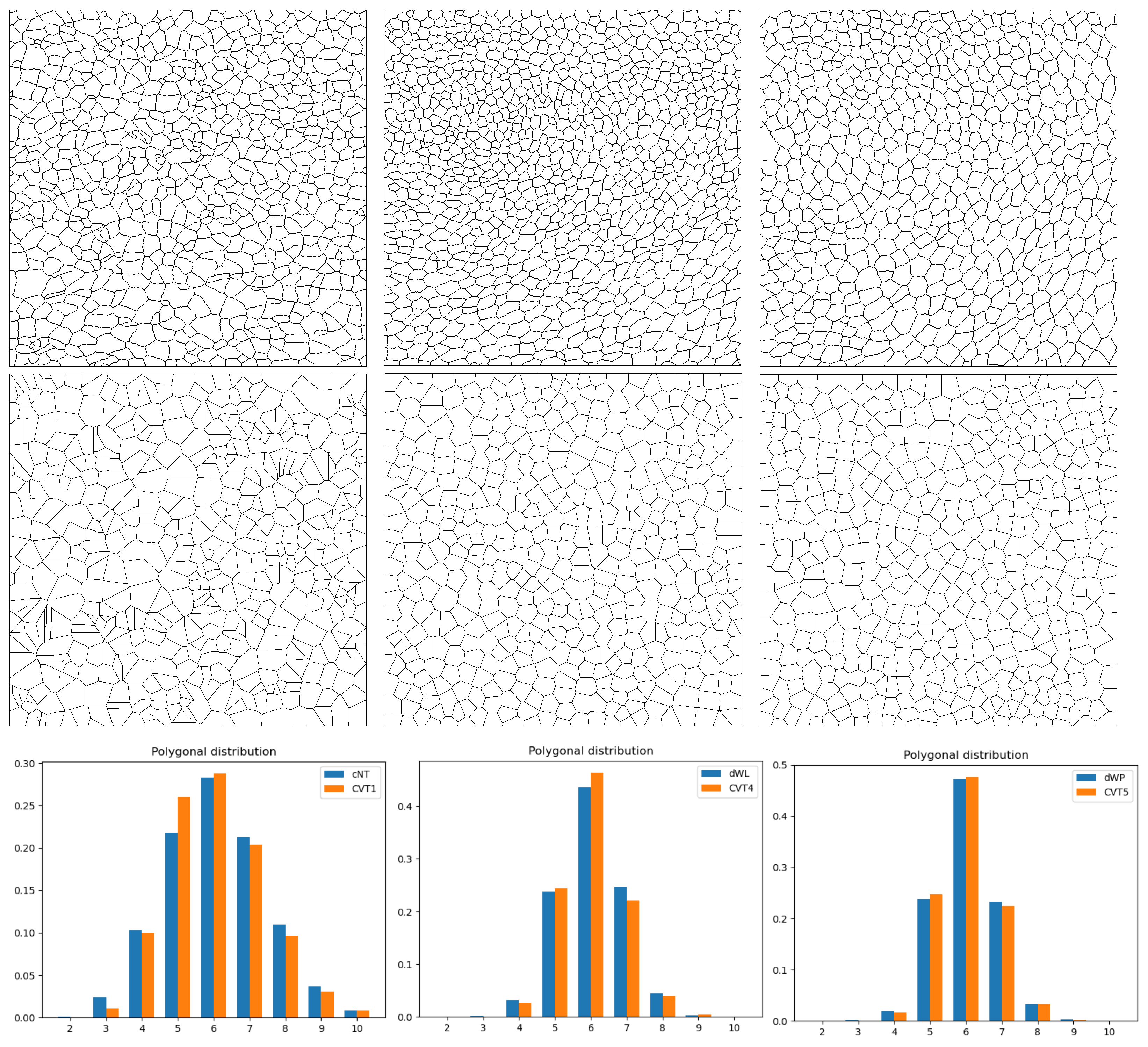
Some of the epithelial tissues were compared with their most similar tessellation in the CVT-path. Following [7], cNT follows a similar neighbor distribution to , dWL to , and dWP to , see Figure 6.
Since we are only interested in making those pairwise comparisons, we performed the Mann–Whitney U test instead of the Kruskall–Wallis test. The minimum valid cells per image is 257 (see Table 1). A selection of the results are displayed in Table 4. Many variables follow different distributions between the CVT tissue and its epithelium counterpart (between 8 and 17 depending on the type compared), most of them in the rips filtration. Differences in the sub and sup filtrations were only found between cNT and .
3.2. Classifying the Images
We classified the epithelial images into three classes: cEE, cNT, and Drosophila tissues. Drosophila tissues are dWL, dWP, and dNP. These tissues can be easily separated from and using the mean and variance of the degrees in the contact graph. Nevertheless, distinguishing between cEE and cNT is more difficult. Since we do not have a big sample of data, we will use the Random Forest technique to avoid over-fitting. Many variables used in network analysis have a strong relation with the mean degree in this specific context ([8], Section 8.2.2). Then, variables used for the network analysis are: the mean and variance of the degree and the amount of cells with degree equal to cells. We fixed as in the first experiment of Section 3.1. We used of data as a training test and for validation. We fixed the number of trees at 200 since the accuracy is already stabilized for that number. This procedure was repeated times, and the average accuracy of the classification is shown in Table 5. The best result was reached with only 3 variables: the mean and variance of the degree and . The validation results were slightly better than the training ones, so we did not commit to over-fitting. The selected variables outperformed the others. This proves that the TDA variable may be useful to complement other variables in machine learning tasks.
3.3. Interpretation of the Variables
As we will see, information carried by sub and sup filtration is strongly related with the neighbor distribution, but not only, since details of the inner organization of the tissue might enrich it.
Besides, rips is strongly related with the relative proximity of the centroids of the cells inside the same image and any interpretation of a variable must be within those terms.
In the following, we will use the term n-cell to refer to a cell with n neighbors.
3.3.1. The Variable
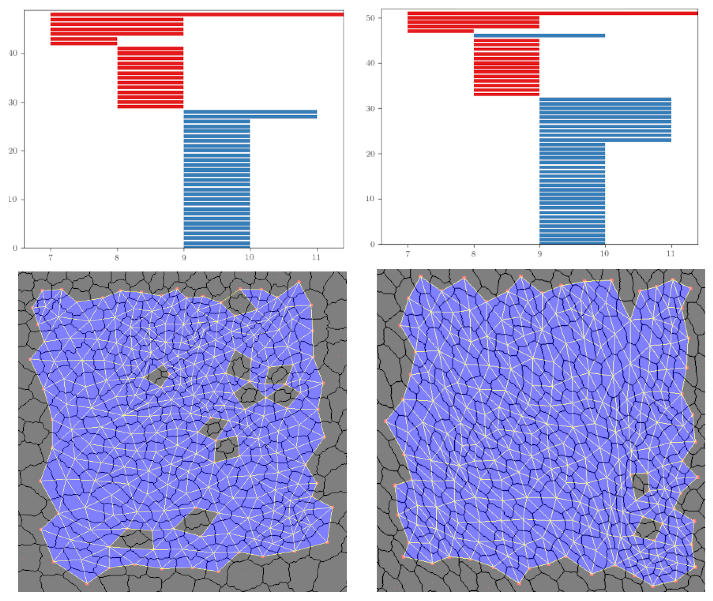
This variable is measuring for which filtration values there are at least k 1-dimensional holes simultaneously “alive”. For , we obtained that the most discriminating value of k was , see Figure 7. 1-dimensional holes in the sub filtration are formed when there are clusters of cells surrounded by other cells with a smaller amount of neighbors, see Figure 2. For example, cEE has a big variance with more cells with few neighbors (2 or 3) or many neighbors (8 or 9) compared to other tissues. In particular, cells with more neighbors have a greater chance to appear forming clusters than in other tissues, where it is more common to find them isolated. Then, a smaller number of 1-dimensional holes is expected. There is another factor, cEE cells are far from being convex, allowing settings such as isolated small cells embedded between two or three big cells. Therefore, again, 1-dimensional holes in cEE are less likely than in other tissues, and never reach the 9 simultaneous 1-dimensional holes threshold.
On the other hand, Drosophila images have small variance with plenty of cells with 6 neighbors. In particular, when , all 6-cells are connected and many 1-dimensional holes appear, one for each cluster formed by cells with more than 6 neighbors, see Figure 2. Finally, cNT is halfway of both.
In general, there is a strong correlation between this variable and the variance of the degrees. For the rest of the variables, complementary information will become more important than just the degree distributions.
3.3.2. The Variable
In this case, landscape is measuring for which interval values there are at least k connected components simultaneously alive. In our experiment, the best k is . An interesting pattern arises, which improves the results with respect to just using the number of neighbors. Many cells with 2 or 3 neighbors are just cells on the boundary which will be connected soon with some neighbor. Nevertheless, cEE tissues have non-boundary cells with 2 or 3 neighbors which are isolated and surrounded by cells with 6 or 7 neighbors. This will generate some longer connected components than in the other tissues.
In the other chicken tissue, cNT, cells with degrees from 4 to 8 neighbors are more uniformly distributed in the image. Hence, a greater proportion of connected components arises with birth time 4 or 5 and death time for 6 neighbors.
This effect is even clearer in Drosophila tissues: since there are fewer 4-cells, connected components with 2 or 3 cells on the boundary are alive until cells with 5 neighbors appear. Many of them connect with cells on the boundary, but other 5-cells remain isolated or in small clusters, creating connected components. These new connected components have a short life and usually die when 6-cells appear.
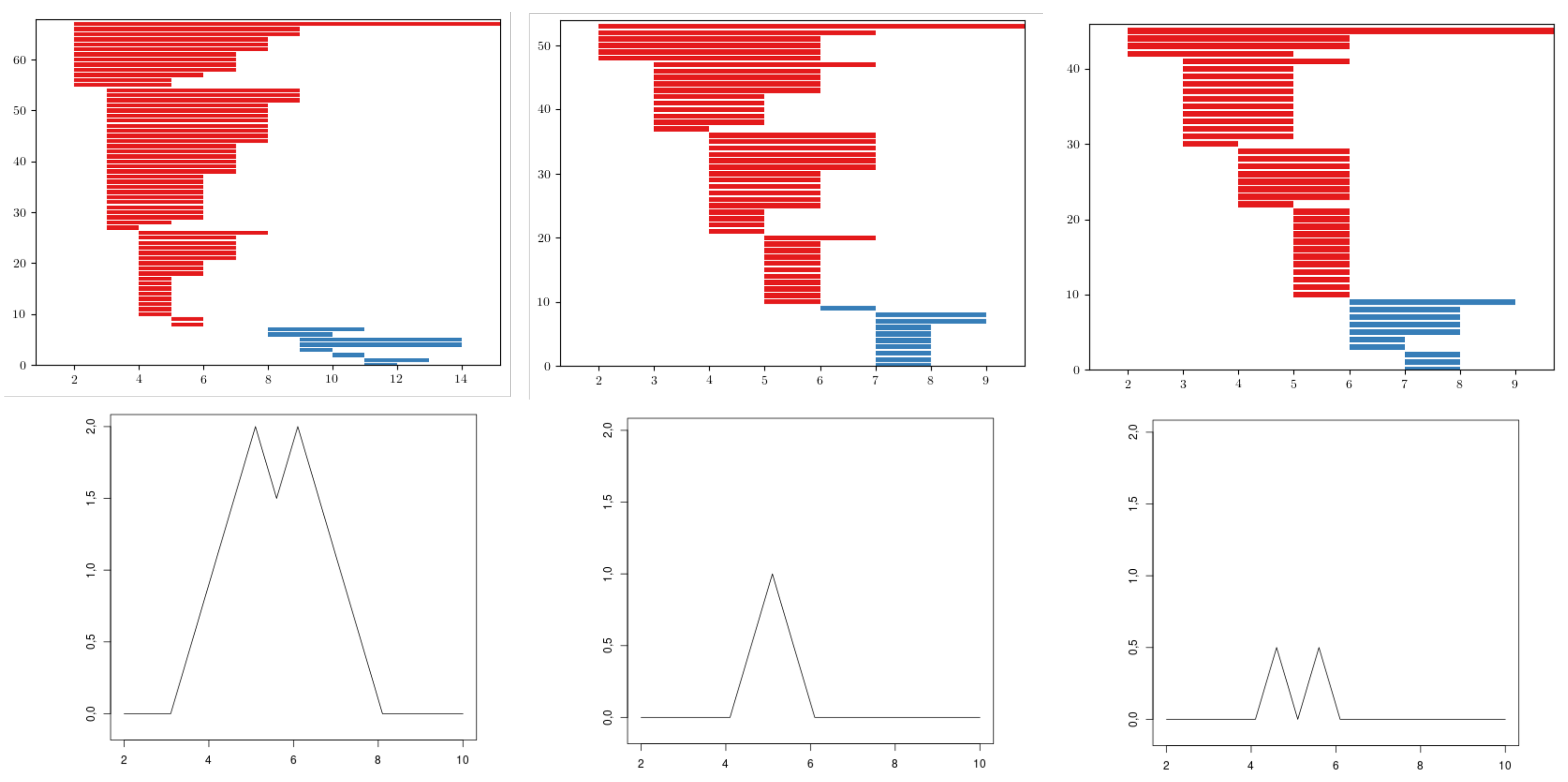
Then, cEE landscape tends to have a greater area with two close peaks, cNT landscape tends to have a medium area with only one peak, and Drosophila landscape tends to have a smaller area and 1 or 2 separated peaks depending on whether there are enough -cells or not, see Figure 8.
Therefore, this variable is not only taking into account the distribution of the cells but also how cells with different numbers of neighbors are connected among them and with regard to the boundary. As it is shown in the Random Forest classification, this variable performs better for classification than directly comparing the number of neighbors (see the accuracy of network variables vs. mean + variance + in Table 5).
3.3.3. and
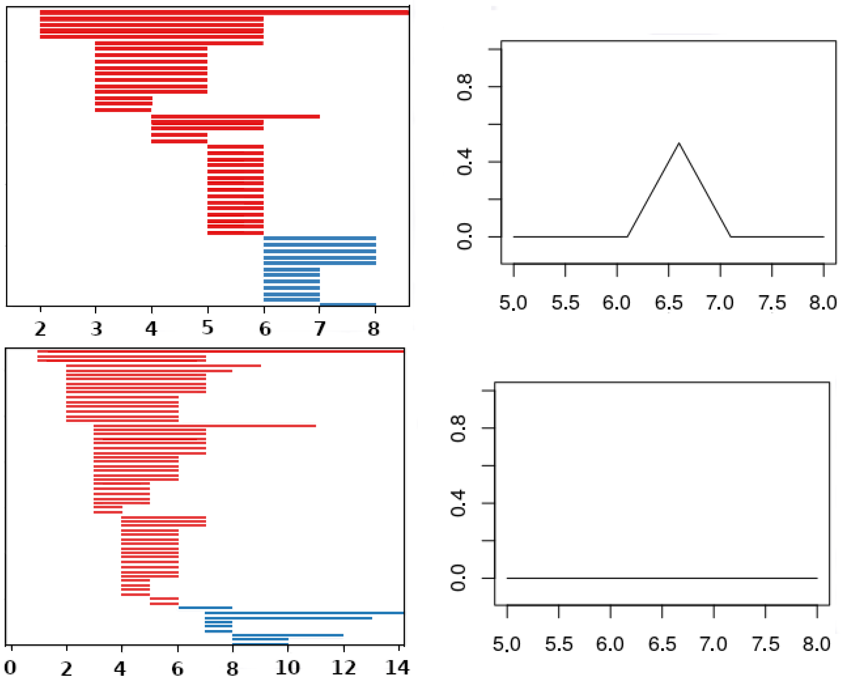
These variables become especially important when comparing dWL and dWP. Actually, in this case, there is a huge correlation between both variables since they are measuring the same feature at the tissue level. 1-dimensional holes in the sup filtrations appear when there are cells (or clusters of cells) with a small number of neighbors which are surrounded by cells with a higher number of neighbors. In this case, the key difference between both tissues is provided by persistence bars, which appear when there are 4-cells, some of whose neighbors are 6- or 7-cells. The presence of this combination of cells provides more bars with longer persistence in dWL than in dWP, see Figure 9. Then, (and the sum ) will be greater in dWL. For , the best result is reached when . In Table 6, we display a small experiment showing that this variable is measuring different features than just the distribution of neighbors.
3.3.4.
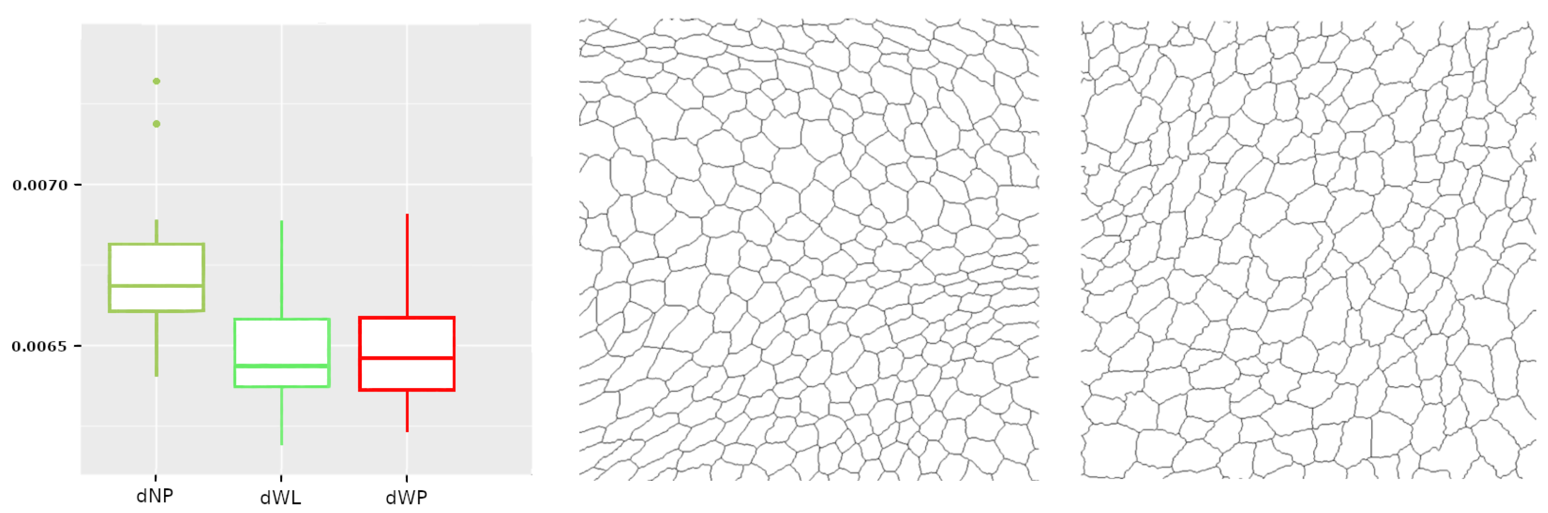
Calculating the length of the k-th longest bar in the rips filtration is equivalent to the distance for which there are less than k connected components. Since our barcodes are normalized, the distance has no units and can be interpreted as a proportion. Besides, in this dataset, the longest bars are associated with connected components corresponding to isolated centroids, or small clusters of centroids (recall that the infinity bar was removed). Then, this variable is directly related with the (relative) distance between the centroids. In practice, it is measuring if there are at least k centroids with a relative distance to the main connected component bigger than the others in the same image. The most discriminating k for is . This type of variable, , becomes important when analyzing Drosophila tissues, since it is the only one finding differences between dNP and the others (dWL, dWP). An example is shown in Figure 10.
3.3.5.
Note that since Shannon entropy is a concave function in the space of probability distribution [30], so is the persistent entropy in the space of normalized rips barcodes. Then, knowing the maximum will give us a valuable hint for understanding this variable at the tissue level.
We will consider a point cloud as a finite metric space, M. Then, we define a distance graph on M, , as a clique graph whose set of vertices is given by a point cloud and the weight on each edge is the distance between the corresponding vertices.
Proposition 6.
Let M be a finite metric space and its persistence barcode (with the infinity bar removed) coming from its rips filtration. Then, is maximum if and only if the minimum spanning tree of its distance graph, , has a constant weight for all its edges.
Proof.
Note that since we only consider the 0-dimensional rips barcode, all bars are born at 0 and their death value is the same as their length. Besides, note that Shannon entropy reaches its maximum value when all probabilities are the same [30]. Then, persistent entropy reaches its maximum value when all bars have the same length. Combining these two facts, we can see that persistent entropy will be maximum if and only if all bars have the same death value. One direction is clear: If the minimum spanning tree has a constant weight, it means that all the vertices are isolated until the filtration value reaches that constant. Then, all the finite bars die at that value. For proving the other direction, assume that the minimum spanning tree does not have a constant weight and define w as its minimum weight. When the filtration value is w, some of the vertices become connected between them, but not all of them. This means that some bars die at w, but some will die later. Then, persistent entropy cannot be maximum. □
Then, is strongly related with the variability of the weights in the minimum spanning tree of the distance graph. It makes sense since entropy may also be understood as a diversity index. In particular, it may have an interpretation in terms of how centroids of the cells are related between them. This variable becomes especially important when comparing some tissues with their CVT counterpart, since it was the only one (together with ) succeeding in differentiating all the cases, see Table 4. Then, it means that the CVT-path fails to imitate the centroid distribution of the cells.
4. Discussion
Here, we summarize the results of this paper. Normalizing the number of cells obtained from each tissue, as well as the rips barcodes, allowed us to compare the network and centroid distributions of different cell tissues without losing stability properties. This was proven by some theoretical results appearing in Section 2.6 and Section 2.7. Note that these results may be generalized with respect to other tessellations of the plane. In Section 3, we compared some epithelia, obtaining some conclusions that might be of interest for the biological community:
- The geometry of the cells in cEE and cNT are completely different (cNT cells tend to be convex, while cEE do not), and so is their contact network. Nevertheless, their centroid distributions turned out to be very similar. Is there any biological or physical reason for this fact?
- Wing tissues in larva (dWL) and prepupa (dWP) stages of development are difficult to differentiate, although it is known that the tissue follows a more regular/hexagonal packing in the pupa stage [5], which is a more advanced stage than dWL and dWP. We noticed that the variable and worked pretty well when differentiating dWL from dWP. The main reason was a difference in the number of 4-cells surrounded by a mix of 6- and 7-cells, which is greater in the dWP case. This might be due to the transition from the polygonal distribution in dWL (with of hexagons) to the one of the pupa stage (with nearly ) [1]. This could be a clearer and simpler indicator of the state of development than the one used in [5].
- Some diagrams of the CVT-path have a similar polygon distribution to some natural tissues according to [7]. In particular, they find similarities between and cNT, and dWL, and and dWP. In this paper, we were able to find differences between the contact network of and cNT. In addition, we found differences between the centroid distribution of the natural tissues and their CVT counterparts. This indicates a limitation of CVT-paths as models of natural packed tissues and might help to find better ones in the future.
There are also interesting results for the pattern recognition community:
- We provided an example where TDA may be useful to study networks with a very simple topology, leading to the study of variables which would have been difficult to discover otherwise.
- In particular, we proposed a combination of normalization in the original image and in the barcode, which allows to prove the formal stability of the method.
- This paper also provided an example where TDA variables may be combined with others to improve machine learning performance.
In comparison with other authors working on the same database, we would like to highlight the following points:
- Results in [8] constitute a preliminary study, the author finds differences using PCA methods, and obtained results similar to the one obtained using the mean and variance of the degree in the contact network. In particular, no results separating tissues with similar mean and variance of the degree are provided. We are able to find significant differences in that situation, for example between dWL, dWP, and dNP.
- In [8], the author points out the similarity of cNT to a randomly generated model. In [7], a similar result is obtained. The authors compare the cNT tissues with respect to (the Voronoi Diagram of a point cloud generated by a Poisson distribution), which is also a random model. In this paper, we were able to find significant differences between cNT and at both levels, its contact network and spatial distribution of the centroids. Then, we were able to describe it using stable topological summaries and to prove that it is definitely different to .
- Besides, in [7], no differences between the polygon distributions of dWL and and dWP and were found. Our work reinforces these results since we did not find significant differences on the contact network. Nevertheless, we found significant differences between the spatial distribution of their centroids. This supports the claim of [10], that the inner structure of epithelia cannot be completely described just using the contact network, but requires spatial information.
- The tool in [4] is not able to distinguish between dWL and dWP. We detected that the number of 4-cells with neighbors formed by 6- and 7-cells can differentiate both tissues. Note that this structure is not a graphlet, since graphlets do not contain information about the degree of the cells in the contact graph.
5. Conclusions and Future Work
We have proven that TDA is a powerful tool to quantify the contact network and the spatial distribution of cells in a packed tissue. We have also carried out a theoretical analysis which guarantees that our method:
- is stable,
- measures different information to usual polygonal distribution,
- provides an interpretation available for many of the variables.
On the other hand, our method requires to extract a fixed number of cells from each image, which might make the experiment computationally more expensive.
In [8], polygons were glued following some topological constraints to generate random surfaces, which could be used as models of epithelial tissues. A future work could be to create new models of epithelial tissues by imposing some specific values on our variables. For example, we believe that can be especially useful in this context. Following this procedure, we expect to obtain more realistic models, adding spatial correlation properties, as pointed out in [10]. In addition, we expect that this tool may help the biological community to understand aspects of morphogenesis that are not explicitly directed by genetic control [1]. Note that we have only worked with apical surfaces of epithelial tissues. Another interesting direction is to adapt our analysis to 3D epithelium, which is nowadays a very active research field [33], as well as to other fields, such as material science [34].
Author Contributions
Investigation, N.A., M.-J.J. and M.S.-T. All authors have read and agreed to the published version of the manuscript.
Funding
This research was funded by Ministerio de Ciencia e Innovación—Agencia Estatal de Investigación/10.13039/501100011033, grant number PID2019-107339GB-I00. The author M. Soriano-Trigueros was partially funded by the grant VI-PPITUS from the University of Seville.
Institutional Review Board Statement
Not applicable.
Informed Consent Statement
Not applicable.
Data Availability Statement
Publicly available datasets were analyzed in this study. This data, together with the whole code from the experiment, can be found here: github.com/Cimagroup/topo-summaries-for-packed-tissues (accessed on 18 May 2021).
Acknowledgments
The authors would like to thank the researchers L.M. Escudero, P. Gómez-Gálvez, and C. Molero-Ríos for their valuable help during the development of this research.
Conflicts of Interest
The authors declare no conflict of interest.
Abbreviations
The following abbreviations were used in this manuscript:
| TDA | Topological data analysis |
| CVT | Centroidal Voronoi tessellation |
| cEE | Chick quamousembryonic ectoderm |
| cNT | Chick neuroepithelium |
| dNP | Drosophila prepupal notum |
| dWL | Drosophila larva wing discs |
| dWP | Drosophila prepupal wing discs |
References
- Gibson, W.T.; Gibson, M.C. Chapter 4 Cell Topology, Geometry, and Morphogenesis in Proliferating Epithelia. In Current Topics in Developmental Biology; Academic Press: Cambridge, MA, USA, 2009; Volume 89, pp. 87–114. [Google Scholar] [CrossRef]
- Emmanuele, V.; Kubota, A.; Garcia-Diaz, B.; Garone, C.; Akman, H.O.; Sánchez-Gutiérrez, D.; Escudero, L.M.; Kariya, S.; Homma, S.; Tanji, K.; et al. Fhl1 W122S causes loss of protein function and late-onset mild myopathy. Hum. Mol. Genet. 2014, 24, 714–726. [Google Scholar] [CrossRef] [Green Version]
- Park, J.A.; Kim, J.H.; Bi, D.; Mitchel, J.A.; Qazvini, N.T.; Tantisira, K.; Park, C.Y.; McGill, M.; Kim, S.H.; Gweon, B.; et al. Unjamming and cell shape in the asthmatic airway epithelium. Nat. Mater. 2015, 14, 1040–1048. [Google Scholar] [CrossRef]
- Vicente-Munuera, P.; Gomez-Galvez, P.; Tetley, R.; Forja, C.; Tagua, A.; Letran, M.; Tozluoglu, M.; Mao, Y.; Escudero, L. EpiGraph: An open-source platform to quantify epithelial organization. Bioinformatics 2019, 36, 1314–1316. [Google Scholar] [CrossRef] [PubMed] [Green Version]
- Sánchez-Gutiérrez, D.; Sáez, A.; Pascual, A.; Escudero, L. Topological Progression in Proliferating Epithelia Is Driven by a Unique Variation in Polygon Distribution. PLoS ONE 2013, 8, e79227. [Google Scholar] [CrossRef] [PubMed] [Green Version]
- Emelianenko, M.; Ju, L.; Rand, A. Nondegeneracy and Weak Global Convergence of the Lloyd Algorithm in Rd. SIAM J. Numer. Anal. 2008, 46, 1423–1441. [Google Scholar] [CrossRef]
- Sánchez-Gutiérrez, D.; Tozluoglu, M.; Barry, J.D.; Pascual, A.; Mao, Y.; Escudero, L.M. Fundamental physical cellular constraints drive self-organization of tissues. EMBO J. 2016, 35, 77–88. [Google Scholar] [CrossRef]
- Villoutreix, P. Randomness and Variability in Animal Embryogenesis, A Multi-Scale Approach. Ph.D. Thesis, Université Sorbonne Paris Cité, Paris, France, 2015. [Google Scholar]
- Churkin, A.; Totzeck, F.; Zakh, R.; Parr, M.; Tuller, T.; Frishman, D.; Barash, D. A Mathematical Analysis of RNA Structural Motifs in Viruses. Mathematics 2021, 9, 585. [Google Scholar] [CrossRef]
- Sandersius, S.; Chuai, M.; Weijer, C.; Newman, T. Correlating Cell Behavior with Tissue Topology in Embryonic Epithelia. PLoS ONE 2011, 6, e18081. [Google Scholar] [CrossRef]
- Edelsbrunner, H.; Letscher, D.; Zomorodian, A. Topological Persistence and Simplification. Discret. Comput. Geom. 2002, 28, 511–533. [Google Scholar] [CrossRef] [Green Version]
- Zomorodian, A.; Carlsson, G. Computing Persistent Homology. Discret. Comput. Geom. 2004, 33, 249–274. [Google Scholar] [CrossRef] [Green Version]
- Qaiser, T.; Tsang, Y.W.; Taniyama, D.; Sakamoto, N.; Nakane, K.; Epstein, D.; Rajpoot, N. Fast and accurate tumor segmentation of histology images using persistent homology and deep convolutional features. Med. Image Anal. 2019, 55, 1–14. [Google Scholar] [CrossRef] [Green Version]
- Merelli, E.; Rucco, M.; Sloot, P.; Tesei, L. Topological Characterization of Complex Systems: Using Persistent Entropy. Entropy 2015, 17, 6872–6892. [Google Scholar] [CrossRef] [Green Version]
- Rucco, M.; Viticchi, G.; Falsetti, L. Towards Personalized Diagnosis of Glioblastoma in Fluid-Attenuated Inversion Recovery (FLAIR) by Topological Interpretable Machine Learning. Mathematics 2020, 8, 770. [Google Scholar] [CrossRef]
- Belchi, F.; Pirashvili, M.; Conway, J.; Bennett, M.; Djukanovic, R.; Brodzki, J. Lung Topology Characteristics in patients with Chronic Obstructive Pulmonary Disease. Sci. Rep. 2018, 8, 5341. [Google Scholar] [CrossRef] [PubMed]
- Kališnik, S. Tropical Coordinates on the Space of Persistence Barcodes. Found. Comput. Math. 2018, 101–129. [Google Scholar] [CrossRef] [Green Version]
- Jimenez, M.J.; Rucco, M.; Vicente-Munuera, P.; Gómez-Gálvez, P.; Escudero, L.M. Topological Data Analysis for Self-organization of Biological Tissues. In Proceedings of the Combinatorial Image Analysis: 18th International Workshop, IWCIA 2017, Plovdiv, Bulgaria, 19–21 June 2017; pp. 229–242. [Google Scholar] [CrossRef]
- Atienza, N.; González-Díaz, R.; Soriano-Trigueros, M. On the stability of persistent entropy and new summary functions for topological data analysis. Pattern Recognit. 2020, 107, 107509. [Google Scholar] [CrossRef]
- Atienza, N.; Escudero, L.M.; Jimenez, M.J.; Soriano-Trigueros, M. Characterising Epithelial Tissues Using Persistent Entropy. In Computational Topology in Image Context; Springer International Publishing: Berlin/Heidelberg, Germany, 2018; pp. 179–190. [Google Scholar] [CrossRef] [Green Version]
- Edelsbrunner, H.; Harer, J. Computational Topology: An introduction; American Mathematical Society: Providence, RI, USA, 2010. [Google Scholar]
- Bhaskar, D.; Zhang, W.Y.; Wong, I.Y. Topological Data Analysis of Collective and Individual Epithelial Cells using Persistent Homology of Loops. arXiv 2021, arXiv:q-bio.QM/2003.10008. [Google Scholar]
- Aukerman, A.; Carrière, M.; Chen, C.; Gardner, K.; Rabadán, R.; Vanguri, R. Persistent Homology Based Characterization of the Breast Cancer Immune Microenvironment: A Feasibility Study. In Proceedings of the 36th International Symposium on Computational Geometry (SoCG 2020), Zürich, Switzerland, 23–26 June 2020; Cabello, S., Chen, D.Z., Eds.; Schloss Dagstuhl–Leibniz-Zentrum für Informatik: Dagstuhl, Germany, 2020; Volume 164, pp. 11:1–11:20. [Google Scholar] [CrossRef]
- Escudero Cuadrado, L.M.; da Fontoura Costa, L.; Kicheva, A.; Briscoe, J.; Freeman, M.; Babu, M.M. Epithelial organisation revealed by a network of cellular contacts. Nat. Commun. 2011, 2. [Google Scholar] [CrossRef] [PubMed] [Green Version]
- Kaliman, S.; Jayachandran, C.; Rehfeldt, F.; Smith, A.S. Limits of Applicability of the Voronoi Tessellation Determined by Centers of Cell Nuclei to Epithelium Morphology. Front. Physiol. 2016, 7. [Google Scholar] [CrossRef] [Green Version]
- Lloyd, S. Least squares quantization in PCM. IEEE Trans. Inf. Theory 1982, 28, 129–137. [Google Scholar] [CrossRef]
- Mileyko, Y.; Mukherjee, S.; Harer, J. Probability measures on the space of persistence diagrams. Inverse Probl. 2011, 27, 124007. [Google Scholar] [CrossRef] [Green Version]
- Chintakunta, H.; Gentimis, T.; Gonzalez-Diaz, R.; Jimenez, M.; Krim, H. An entropy-based persistence barcode. Pattern Recognit. 2015, 48, 391–401. [Google Scholar] [CrossRef]
- Rucco, M.; Castiglione, F.; Merelli, E.; Pettini, M. Characterisation of the Idiotypic Immune Network Through Persistent Entropy. In Proceedings of ECCS 2014; Springer International Publishing: Berlin/Heidelberg, Germany, 2016; pp. 117–128. [Google Scholar] [CrossRef]
- Cover, T.; Thomas, J. Elements of Information Theory, 2nd ed.; Wiley Series in Telecommunications and Signal Processing; John Wiley & Sons: Hoboken, NJ, USA, 2006. [Google Scholar]
- Bubenik, P. Statistical Topological Data Analysis Using Persistence Landscapes. J. Mach. Learn. Res. 2015, 16, 77–102. [Google Scholar]
- Bubenik, P. The Persistence Landscape and Some of Its Properties. Topol. Data Anal. Abel Symp. 2020, 15, 97–117. [Google Scholar] [CrossRef]
- Gómez-Gálvez, P.; Vicente-Munuera, P.; Anbari, S.; Buceta, J.; Escudero, L.M. The complex three-dimensional organization of epithelial tissues. Development 2021, 148. [Google Scholar] [CrossRef]
- Hiraoka, Y.; Nakamura, T.; Hirata, A.; Escolar, G.; Matsue, K.; Nishiura, Y. Hierarchical structures of amorphous solids characterized by persistent homology. Proc. Natl. Acad. Sci. USA 2016, 113, 7035–7040. [Google Scholar] [CrossRef] [Green Version]
Figure 1.
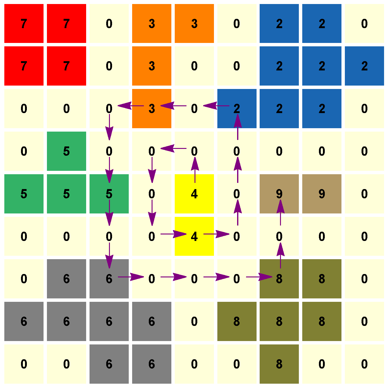
Algorithm 1 runs over the pixels following a spiral until the desired number of labels (of cells) is reached. In this toy example, taking as input parameter , the output is the set of labels . Boundary pixels are labeled by 0.
Figure 1.
Algorithm 1 runs over the pixels following a spiral until the desired number of labels (of cells) is reached. In this toy example, taking as input parameter , the output is the set of labels . Boundary pixels are labeled by 0.

Figure 2.
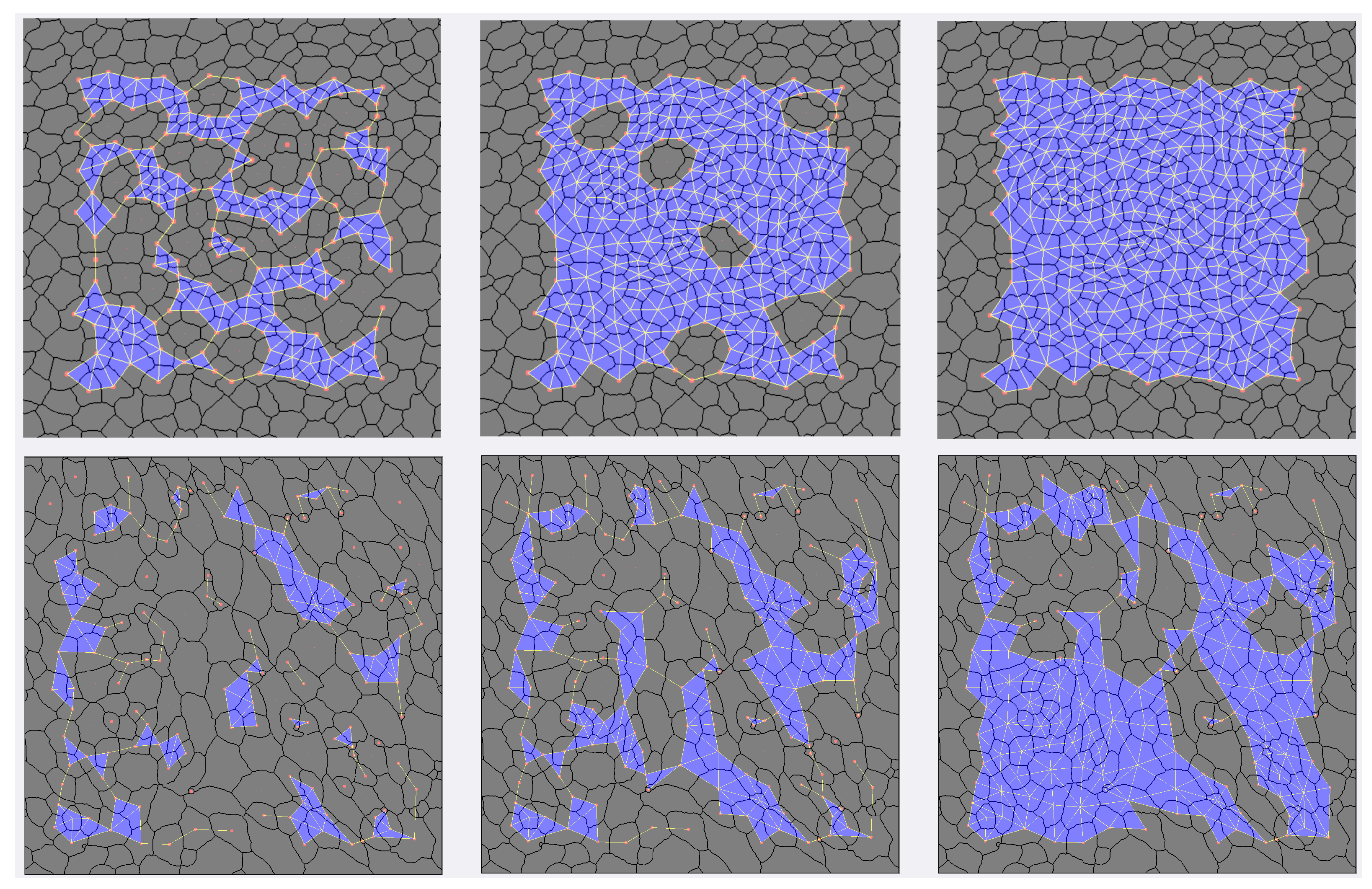
An example of the sub filtration for . The top row corresponds to dNP and the bottom to cEE.
Figure 2.
An example of the sub filtration for . The top row corresponds to dNP and the bottom to cEE.

Figure 3.
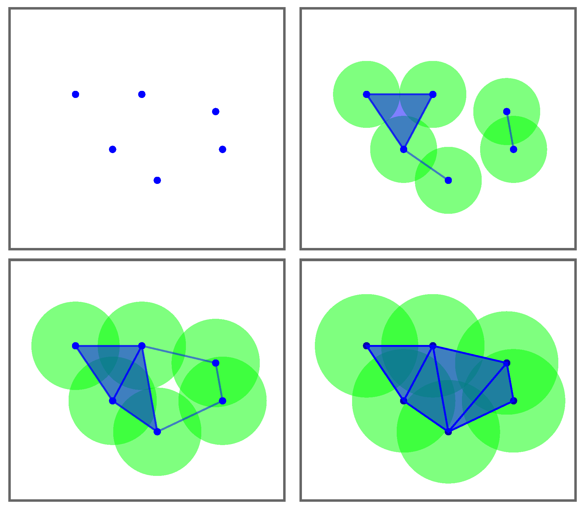
An example of a rips filtration with 6 points in the Euclidean plane. Note that a simplex arises when the distance between the corresponding centroids is smaller than or equal to twice the radius.
Figure 3.
An example of a rips filtration with 6 points in the Euclidean plane. Note that a simplex arises when the distance between the corresponding centroids is smaller than or equal to twice the radius.

Figure 4.
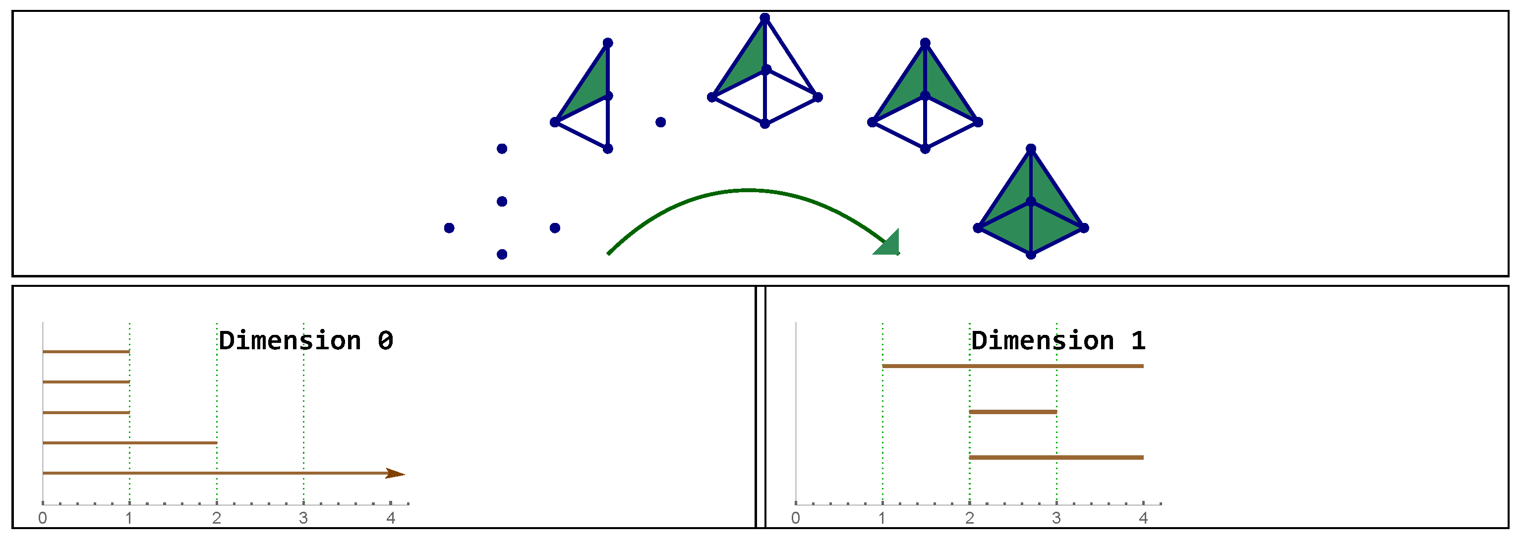
Top: example of a filtration . Bottom: barcodes representing connected components and cycles. Note there is a bar in the 0 dimensional persistent homology. In this example: and then appears once in the 1-dimensional barcode.
Figure 4.
Top: example of a filtration . Bottom: barcodes representing connected components and cycles. Note there is a bar in the 0 dimensional persistent homology. In this example: and then appears once in the 1-dimensional barcode.

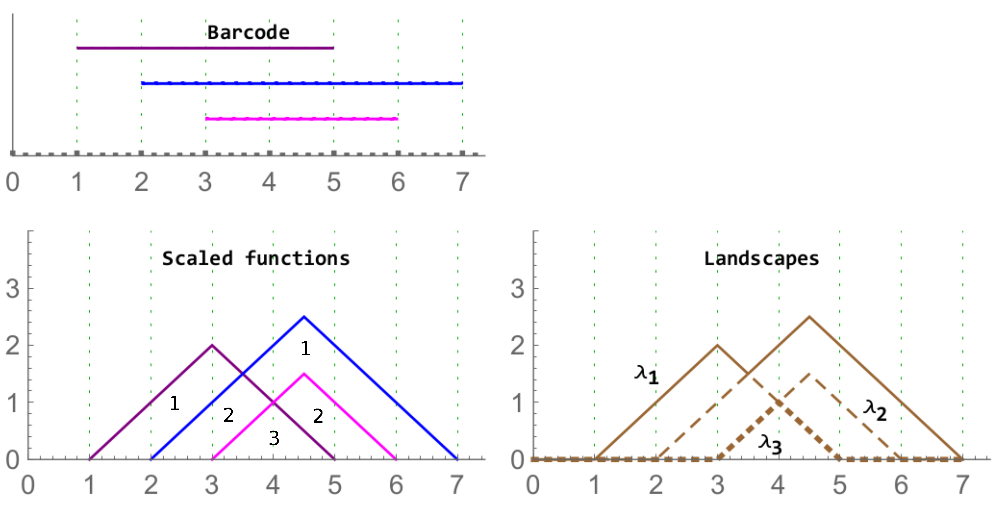
Figure 5.
Left column: A barcode (top) and its corresponding rescaled rank functions (bottom). The values of the functions in the corresponding region are provided. On the right, the associated landscape with the functions , , and are displayed with different layouts.
Figure 5.
Left column: A barcode (top) and its corresponding rescaled rank functions (bottom). The values of the functions in the corresponding region are provided. On the right, the associated landscape with the functions , , and are displayed with different layouts.

Figure 6.
An example of images of epithelial tissues (top row), their CVT-path counterpart (middle row), and a histogram with their polygonal distribution (bottom row). In the first column, we show cNT and ; in the second, dWL and , and in the third, and .
Figure 6.
An example of images of epithelial tissues (top row), their CVT-path counterpart (middle row), and a histogram with their polygonal distribution (bottom row). In the first column, we show cNT and ; in the second, dWL and , and in the third, and .

Figure 7.
An example of barcodes (0-bars in red and 1-bars in blue) with their landscape . The top corresponds to dNP and the bottom to cEE. Note that in the cEE case, there are not 9 1-dimensional holes simultaneously alive, so its landscape is zero.
Figure 7.
An example of barcodes (0-bars in red and 1-bars in blue) with their landscape . The top corresponds to dNP and the bottom to cEE. Note that in the cEE case, there are not 9 1-dimensional holes simultaneously alive, so its landscape is zero.

Figure 8.
An example of barcodes and its landscapes from cEE, cNT, and dWL, respectively. Note that the domain of the landscapes of cNT and dWL are the same, but the area of cNT is greater, since in that domain the 18 bars are the same, while for dWL the bars vary.
Figure 8.
An example of barcodes and its landscapes from cEE, cNT, and dWL, respectively. Note that the domain of the landscapes of cNT and dWL are the same, but the area of cNT is greater, since in that domain the 18 bars are the same, while for dWL the bars vary.

Figure 9.
An example with the persistence barcodes of dWL and dWP, which provide the median for and their corresponding sup filtration when i = 10.
Figure 9.
An example with the persistence barcodes of dWL and dWP, which provide the median for and their corresponding sup filtration when i = 10.

Figure 10.
On the left, the boxplot corresponds to . On the right are the images of dNP and dWL, which provide the median for each of these sets of images.
Figure 10.
On the left, the boxplot corresponds to . On the right are the images of dNP and dWL, which provide the median for each of these sets of images.


Table 1.
The number of valid cells in each image of the epithelial tissues.
| 1 | 2 | 3 | 4 | 5 | 6 | 7 | 8 | 9 | 10 | 11 | 12 | 13 | 14 | 15 | 16 | |
|---|---|---|---|---|---|---|---|---|---|---|---|---|---|---|---|---|
| cEE | 140 | 206 | 229 | 241 | 385 | 380 | 261 | 187 | 405 | 246 | 327 | 204 | 348 | 270 | ||
| cNT | 666 | 661 | 566 | 574 | 669 | 532 | 420 | 592 | 744 | 527 | 594 | 473 | 704 | 748 | 469 | 834 |
| dNP | 513 | 723 | 588 | 525 | 439 | 823 | 1102 | 533 | 309 | 575 | 302 | 375 | ||||
| dWL | 432 | 556 | 485 | 525 | 501 | 936 | 890 | 790 | 977 | 913 | 606 | 835 | 785 | 748 | 622 | |
| dWP | 748 | 806 | 566 | 415 | 454 | 654 | 752 | 713 | 504 | 430 | 387 | 516 | 419 | 455 | 277 | 257 |
Table 2.
Differences between the tissues for 187 cells. A check mark implies that the p-value of that variable is smaller than in the Dunn test and a cross mark that we could not find significant differences using that variable.
Table 2.
Differences between the tissues for 187 cells. A check mark implies that the p-value of that variable is smaller than in the Dunn test and a cross mark that we could not find significant differences using that variable.
| 187 Cells | |||||
|---|---|---|---|---|---|
| cEE vs. cNT | √ | × | × | × | × |
| cEE vs. dNP | √ | × | √ | × | √ |
| cNT vs. dNP | √ | × | √ | × | × |
| cEE vs. dWL | √ | × | √ | √ | √ |
| cNT vs. dWL | × | × | √ | √ | √ |
| dNP vs. dWL | × | × | × | √ | × |
| cEE vs. dWP | √ | √ | √ | √ | √ |
| cNT vs. dWP | × | √ | √ | √ | √ |
| dNP vs. dWP | × | × | × | √ | √ |
| dWL vs. dWP | × | √ | × | × | × |
Table 3.
The p-values of some variables for the Mann–Whitney U test between dWL and dWP. The number of cells is set at 187 and 257.
Table 3.
The p-values of some variables for the Mann–Whitney U test between dWL and dWP. The number of cells is set at 187 and 257.
| dWL vs. dWP | |||
|---|---|---|---|
| N = 187 | 0.013 | 0.01 | 0.019 |
| N = 257 | 0.012 | 0.006 | 0.005 |
Table 4.
Differences between some tissues and their CVT-path counterpart. A check mark implies that the p-value of that variable is smaller than in the Mann–Whitney U test and a cross mark that we could not find significant differences using that variable.
Table 4.
Differences between some tissues and their CVT-path counterpart. A check mark implies that the p-value of that variable is smaller than in the Mann–Whitney U test and a cross mark that we could not find significant differences using that variable.
| 257 Cells | ||||
|---|---|---|---|---|
| cNT vs. | √ | √ | √ | √ |
| dWL vs. | × | √ | √ | × |
| dWP vs. | × | √ | × | √ |
Table 5.
Classification of tissues using all TDA variables, all network variables, all variables together, mean and variance of the degree, and a combination of these two with . The accuracy for the training/validation sets are displayed. Best results are in bold.
Table 5.
Classification of tissues using all TDA variables, all network variables, all variables together, mean and variance of the degree, and a combination of these two with . The accuracy for the training/validation sets are displayed. Best results are in bold.
| 187 Cells | TDA | Network | Mixed | m & v | m & v & |
|---|---|---|---|---|---|
| cEE | 85.5/86.7 | 86.2/87.8 | 86.1/87.8 | 89.7/94.3 | 97.1/98.7 |
| cNT | 82.6/83 | 93.4/93.7 | 92.2/92.9 | 89.2/89.7 | 96.2/97.7 |
| Drosophila | 99.7/99.8 | 100/100 | 100/100 | 100/100 | 100/100 |
| overall | 92.9/93.4 | 95.8/96.1 | 95.5/96 | 95.5/96.2 | 98.6/99 |
Table 6.
Classification using Random Forests of the epithelial tissues. On the left, results using the number of neigbors and mean and variance of the degree. Best results are in bold. It can be seen that performs better.
Table 6.
Classification using Random Forests of the epithelial tissues. On the left, results using the number of neigbors and mean and variance of the degree. Best results are in bold. It can be seen that performs better.
| 257 Cells | Network | |
|---|---|---|
| dWL | 63.8/67.4 | 59.9/59.9 |
| dWP | 64.9/66.5 | 82.6/82.8 |
| global | 63.1/65.5 | 70/71.8 |
Publisher’s Note: MDPI stays neutral with regard to jurisdictional claims in published maps and institutional affiliations. |
© 2021 by the authors. Licensee MDPI, Basel, Switzerland. This article is an open access article distributed under the terms and conditions of the Creative Commons Attribution (CC BY) license (https://creativecommons.org/licenses/by/4.0/).
Share and Cite
MDPI and ACS Style
Atienza, N.; Jimenez, M.-J.; Soriano-Trigueros, M. Stable Topological Summaries for Analyzing the Organization of Cells in a Packed Tissue. Mathematics 2021, 9, 1723. https://doi.org/10.3390/math9151723
AMA Style
Atienza N, Jimenez M-J, Soriano-Trigueros M. Stable Topological Summaries for Analyzing the Organization of Cells in a Packed Tissue. Mathematics. 2021; 9(15):1723. https://doi.org/10.3390/math9151723
Chicago/Turabian StyleAtienza, Nieves, Maria-Jose Jimenez, and Manuel Soriano-Trigueros. 2021. "Stable Topological Summaries for Analyzing the Organization of Cells in a Packed Tissue" Mathematics 9, no. 15: 1723. https://doi.org/10.3390/math9151723
Note that from the first issue of 2016, this journal uses article numbers instead of page numbers. See further details here.