Forecasting the Volatility of the Cryptocurrency Market by GARCH and Stochastic Volatility

Abstract

This study examines the volatility of nine leading cryptocurrencies by market capitalization—Bitcoin, XRP, Ethereum, Bitcoin Cash, Stellar, Litecoin, TRON, Cardano, and IOTA-by using a Bayesian Stochastic Volatility (SV) model and several GARCH models. We find that when we deal with extremely volatile financial data, such as cryptocurrencies, the SV model performs better than the GARCH family models. Moreover, the forecasting errors of the SV model, compared with the GARCH models, tend to be more accurate as forecast time horizons are longer. This deepens our insight into volatility forecast models in the complex market of cryptocurrencies.

1. Introduction

Understanding the relationships among cryptocurrencies is important for policymakers whose role is to maintain the stability of financial markets as well as for investors whose investment portfolios contain a portion of cryptocurrencies. Cryptocurrency is a non-centralized digital currency that is exchanged between peers without the need of a central government. Bitcoin [1,2], which was the first cryptocurrency, operates with block chain technology with a system of recording information in a way that makes it difficult or impossible to change, hack, or cheat the system. Because the prices of cryptocurrencies have been increased such as speculative investment purposes and/or a digital asset for real use, they have received growing attention from the media, academics, and the finance industry. Since the inception of Bitcoin in 2009, over several thousand alternative digital currencies have been developed, and there have been a number of studies on the analysis of the exchange rates of cryptocurrency [3]. The degree of the return volatility has been regarded as a crucial characteristic of cryptocurrencies for investors including them in their portfolio. The prices of Bitcoin and Ethereum have been rapidly increased so that the last one-year price of Bitcoin was an almost 400 percent increase to USD 40,406 on 15 June 2021 from USD 9451 on 15 June 2020. Since [4,5], empirical investigations of Bitcoin showed that Bitcoin is more characteristic of an asset rather than a currency, and Bitcoin also possesses risk management and hedging capabilities [6]. In order to predict the exchange rates of the Bitcoin electronic currency against the US Dollar, ref. [7] proposed a non-causal autoregressive process with Cauchy errors. The volatility of Bitcoin using monthly return series is higher than that of gold or some foreign currencies in dollars [8].

A number of academic studies have investigated the factors influencing the price and volatility of cryptocurrencies ([9,10,11,12]). Especially, GARCH family models are employed to estimate the time-varying volatility of cryptocurrencies. Ref. [13] proposed the AR-CGARCH model to estimate the volatility of Bitcoin by comparing GARCH models. Ref. [14] looked at the tail behavior of returns of the five major cryptocurrencies (Bitcoin, Ethereum, Ripple, Bitcoin Cash, and Litecoin), using extreme value analysis and estimating VaR and ES as tail risk measures. They found that Bitcoin Cash is the riskiest, while Bitcoin and Litecoin are the least risky cryptocurrencies. Ref. [15] examined more than 1000 GARCH models and suggest the best fitted GARCH model chosen by back-testing VaR and ES as well as an MCS procedure. They claim that standard GARCH models may result in incorrect predictions and could be improved by allowing asymmetries and regime switching. Ref. [16] employs the BEKK GARCH model to estimate time-varying conditional correlations between gold and Bitcoin.

For the volatility, previous studies have employed a variation of GARCH models, while little attention has been paid to methods outside the GARCH family. Refs. [17,18], examples of a few papers in this area, examine the volatility of cryptocurrencies by hiring the stochastic volatility model and finding out that the use of fast-moving autocorrelation function captures the volatility of cryptocurrencies better than smoothly decaying functions. This study sheds light on other statistical methods for better out-of-sample forecasting power, in particular, the SV model. Instead of using traditional approaches to interpret the association and/or causality among the cryptocurrencies, we use the approaches (SV method) described above because of several advantages. First, financial asset returns are generally fat-tailed and have negative skewness, and the residuals obtained from traditional time series analysis such as GARCH and/or VAR may be contaminated by other explainable portions of the volatility of the return series. Second, it is common that financial time series volatility is correlated in a non-Gaussian way. Lastly, because of the occurrence of extreme observations and the complex structure of the dependence among asset returns, traditional approaches often fail to incorporate the influences of asymmetries in individual distributions and in dependence. A copula function introduces a function linking univariate marginal to their multivariate distribution ([19]).

This study contributes to the literature by highlighting the SV model, which shows superior forecasting accuracy compared with GARCH family models studied in prior studies. The SV considers two error processes, but the GARCH model considers a single error term so that the SV model makes a better in-sample fit. The adoption of cryptocurrencies as an alternative investment asset by institutional investors, such as hedge fund investors, has increased significantly in recent years. The cryptocurrency market, which has shown higher volatility than any other assets in the financial market, requires a significant level of risk management from institutional investors and individuals that incorporate them into their investment portfolios. The excellence of forecasting power in our SV model provides implications that it can be used as a better risk management tool than other GARCH family models. Moreover, the forecasting errors of the SV model, compared with the GARCH models, tend to be more accurate as forecast time horizons are longer. Another contribution of our paper to the literature is, rather, to pay attention to the forecasting power of volatility models using cryptocurrency data than measure volatility itself. Finally, by hiring principal component analysis (PCA), this study examines whether a smaller number of factors are able to explain the variation of a large set of cryptocurrencies. This approach may shed light on which group of cryptocurrencies mainly drives the variation of the daily log-return of cryptocurrencies used in the paper. As the crypto market has been gradually accepted into the mainstream of financial markets, the accurate prediction of cryptocurrency return volatility is in more demand by market participants, financial institutions, and government agencies. The approach used in this study sheds light on what models are examined for a more accurate estimate of cryptocurrency volatility.

This paper is organized as follows. Section 2 gives an overview of the existing volatility models, that is, the GARCH and SV methods. Section 3 presents the data analysis and the discussion and conclusion follow in Section 4 and Section 5, respectively.

2. Materials and Methods

In Section 2, we introduce the two different traditional volatility models used in this study to compare the relative efficiency of the models we used. Our study conducts the SV model to forecast unobserved volatility in financial economics; however, there is another class of models that is frequently used. Refs. [20,21] develop the autoregressive conditional heteroscedasticity (ARCH) and generalized ARCH (GARCH) models, respectively. We employ GARCH (1,1) with constant in Mean, Threshold-GARCH (TGARCH) and the Integrated GARCH (IGARCH) models among the family of the GARCH models. The standard GARCH model assumes that positive and negative error terms have a symmetric effect on volatility. It means that good and bad news have the same effect on the volatility in the standard GARCH model. However, this assumption is easily violated in the financial stock market, in that the negative change in the stock market has a bigger effect on the volatility index than a positive change, or vice-versa. Ref. [22] called it a leverage effect. As such, the asymmetric GARCH models were developed for accommodating a leverage effect. The SV model allows for two error processes, while the GARCH model considers a single error term. Therefore, the SV model makes a better in-sample fit ([23]) and thus could provide a better forecast whereas it potentially involves a heavy computational burden.

2.1. GARCH Models

For a log return series $r_t=log\left(\frac{S_t}{S_{t-1}}\right),$ we let $a_t=r_t-E_{t-1}\left[r_t\right]$ be the innovation at time t. All members of the family of GARCH models are obtained from a transformation of the conditional standard deviation, ${\sigma }_t$, determined by the transformation f () of the innovations, $a_t$, and lagged transformed conditional standard deviations. In particular, we employee three transformation models (GARCH, IGARCH, and TGARCH). An extensive discussion on the nested GARCH models is given in [7].

The mean model is chosen to have ARMA(0,0), and we include a mean-constant so that we let $r_t=\mu +{ϵ}_t$ be the innovation at time t where µ is a mean constant. For a log return series, we let $a_t=r_t-E_{t-1}\left[r_t\right]$ be the innovation at time t. Then $a_t$ follows a GARCH (p,q) with constant in mean model if

$$a_t=\sqrt{h_t}{e}_t$$

(1)

$$h_t={\alpha }_0+{\displaystyle \sum }_{i=1}^q{\alpha }_i{a}_{t-i}^2+{\displaystyle \sum }_{i=1}^p{\beta }_i{h}_{t-i}$$

(2)

where ${\alpha }_0>0, {\alpha }_i\ge 0, {\beta }_i\ge 0,$ and $e_t$~ t-Student distribution, which is explained by its 3 parameters, which are the location, scale and shape parameters in Equation (25) from [24]. The GARCH (p,q) model is stationary with a finite variance if ${\displaystyle \sum }_{i=1}^q{\alpha }_i+{\displaystyle \sum }_{i=1}^p{\beta }_i\le 1$. Furthermore, if ${\displaystyle \sum }_{i=1}^q{\alpha }_i+{\displaystyle \sum }_{i=1}^p{\beta }_i=1$, then the GARCH (p,q) process is called IGARCH model [25] which is either non-stationary or have an infinite variance. In order to model persistence of higher volatility, we need an IGARCH (p,q) model with q ≥ 1. The TGARCH model [26] captures the asymmetric effect in the volatility is given by

$$\sqrt{h_t}={\alpha }_0+{\displaystyle \sum }_{i=1}^q{\alpha }_i\left(\left|a_{t-i}\right|-{\eta }_i{a}_{t-i}\right)+{\displaystyle \sum }_{i=1}^p{\beta }_i\sqrt{h_{t-i}}$$

(3)

where the coefficient in the leverage term ${\eta }_i$ satisfies the condition −1 < ${\eta }_i$ < 1.

For the model selection of the GARCH ((p = 1) and (q = 1)) models considered, we used the Akaike Information Criterion (AIC). In addition, this study also considered the t-Student errors to take into account the possible fatness of the distribution tails of $e_t$.

2.2. Stochastic Volatility Model

In the standard SV model framework [27,28], the data returns, r, that are generated from a probability model $f(r|g)$, where $g$ is a vector of volatilities, and this unobserved vector $g$ has a probabilistic structure $f\left(r|\mathsf{\theta }\right),$ where θ is a vector of parameters (see [23,29,30] for details). In the standard form of the model, volatility is modeled as a Gaussian first-order linear autoregressive (AR(1)) process with mean µ in terms of a series of white innovations {E_t} as follows;

$$g_t-\mu =\varphi \left(g_{t-1}-\mu \right)+E_t$$

(4)

where $E_t\backsim iid N\left(0, h_{\eta }\right)$, independent and identically distributed (iid) as normal, and$\left|\varphi \right|$ < 1. A useful feature of Gaussian AR(1) processes is that the marginal distribution is also normal so that

$$g_0~N\left(\mu , \frac{h_{\eta }}{1-{\varphi }^2}\right)$$

(5)

and the returns are given by

$$r_t=\beta \exp \left(\frac{g_t}{2}\right)e_t, e_t~iid N\left(0,1\right)$$

(6)

where {$e_t$} are independent and identically distributed (iid) as standard normal distribution. We denote p_t to be spot price of a financial asset at time t and its one-period return is defined as $r_t=ln\left(\frac{P_t}{P_{t-1}}\right).$ Let $r={\left(r_1,r_2,\dots , r_n\right)}^T$ be a vector of returns with mean zero. The SV model is that each observation r_t is assumed to have its own contemporaneous variance exp($g_t$/2) = $\sqrt{h_t}$ which becomes $g_t=\ln h_t$. The exp($g_t$) is defined as the latent, time-varying volatility that follows a stochastic evolution. The SV model in this paper is given through:

$$r_t|g_t~ N\left(0,\exp \left(g_t\right)\right)$$

(7)

$$g_t|g_{t-1, \mu , \varphi , {\sigma }_{\eta }}~ N\left(\mu +\varphi \left(g_{t-1}-\mu \right),h_{\eta }\right)$$

(8)

$$g_0| \mu , \varphi , \sqrt{h_{\eta }}~ N\left(\mu ,\frac{h_{\eta }}{1-{\varphi }^2}\right)$$

(9)

where $\mathsf{\theta }=\left(\mu , \varphi , \sqrt{h_{\eta }}\right)$ is a vector of parameters so that µ is the level of log-variance, φ is the persistence of log-variance, and σ_η is the volatility of log-variance. The initial state $g_0$ is distributed according to the stationary distribution of the autoregressive process of order one.

Following [29,31] specifies a prior distribution for the parameter vector $\mathsf{\theta }$ choosing independent components for each parameter, $p\left(\mathsf{\theta }\right)=p\left(\mu \right)p\left(\varphi \right)p\left(\sqrt{h_{\eta }}\right)$ where µ follows the usual normal prior $\mu ~ N\left(b_{\mu }, B_{\mu }\right)$. Ref. [32] notes that the prior of µ is usually chosen to be rather uninformative, e.g., through setting $b_{\mu }$ = 0 and $B_{\mu }\ge 100$ for daily log returns. The persistence parameter $\varphi ~ \left(-1, 1\right)$ is chosen so that $\left(\varphi +1\right)/2$ follows the beta distribution B(α, β), implying

$$p\left(\varphi \right)=\frac{1}{2B\left(\alpha , \beta \right)}{\left(\frac{1+\varphi }{2}\right)}^{\alpha -1}{\left(\frac{1-\varphi }{2}\right)}^{\beta -1}$$

(10)

where α and β are positive hyperparameters and $B\left(\alpha ,\beta \right)=\underset{0}{\overset{1}{{\displaystyle \int }}}{t}^{\alpha -1}{\left(1-t\right)}^{\beta -1}dt$. It is obvious that the autoregressive volatility process is stationary because the support of the beta distribution is the interval (−1,1). Its expected value and variance are

$$E\left(\varphi \right)=\frac{2\alpha }{\alpha +\beta }-1 and V\left(\varphi \right)=\frac{4\alpha \beta }{{\left(\alpha +\beta \right)}^2\left(\alpha +\beta -1\right)}$$

(11)

ref. [31] chooses$h_{\eta }$, the volatility of log-variance, such that $h_{\eta }$ follows the hyperparameter $B_{{\sigma }_{\eta }}^{}$ multiplied by ${\chi }^2\left(df=1\right)$. In Section 2.3, we will compare the volatility forecast predictabilities of the models introduced in Section 2.1 and Section 2.2.

2.3. Volatility Forecast Evaluation

In this subsection we carry out empirical exercise to measure predictive accuracy. The SV and GARCH models with observed returns is initially estimated by using our in-sample data. Forecasts are generated at horizons of 3, 5, 10, 20, 30, and 44 days. Then, our out-of-sample data are added to the sample, and the parameters of the model with an individual approach are estimated. The purpose of considering multiple forecast horizons is to see whether our new approach improves the predictive ability of a time series model at all horizons in a large sample. This is done by applying a common loss function which is a logarithmic version of mean square (prediction) error (MSE):

$${\mathrm{MSE}}_k\equiv \frac{1}{n}{\displaystyle \sum }_{t=1}^n{\left(\ln {\sigma }_t^2-h_t\right)}^2 , where k=1, 2$$

(12)

h_t is the estimates of the conditional log-volatility. This loss function with mathematical simplicity is the popular measure to evaluate forecasting performance in the literature (e.g., [11]). We consider two alternative ex post proxies for the conditional volatility such that $\ln {\sigma }_t^2=r_t^2$ and $\ln {\sigma }_t^2=\left|r_t\right|$ which are noted as k = 1, 2, respectively. A smaller average loss is more accurate and, therefore, preferred.

3. Results

For volatility efficiency comparison, nine cryptocurrencies are applied to the models introduced in Section 2. Considering the sensitivity of the time period in predicting the volatility of financial time-series return data such as cryptocurrencies, we examine two different time periods, short-term and long-term periods. The sample consists of the daily log-returns of the nine cryptocurrencies over period 1 (19 August 2018 to 27 November 2018) and period 2 (2 January 2018 to 27 November 2018). The log-returns of Bitcoin (BTC), XRP (XRP), Ethereum (ETH), Bitcoin Cash (BCH), Stellar (XLM), Litecoin (LTC), TRON (TRX), Cardano (ADA), and IOTA (IOTA) are denoted by LBTC, LXRP, LETH, LBCH, LXLM, LLTC, LTRX, LADA, and LMIOTA, respectively. We obtain our data from a financial website (https://coinmarketcap.com/coins/) (accessed on 10 May 2020). Throughout the year of 2018, BTC’s price fluctuated from USD 17,527.00 (6 January 2018) to USD 3820.72 (27 November 2018). The cryptocurrency market had extremely high volatility during the period 2. However, during the second half of the year 2018 (period 1), BTC’s price did not fluctuate from USD 6308.53 (20 August 2018) to USD 3820.72 (27 November 2018) compared with period 2. We can say that the period 1 was low volatile time period and the period 2 was high volatile time period. It is good to perform the comparison of volatile forecasting with the GARCH models and SV model for two low and high volatile cryptocurrency data.

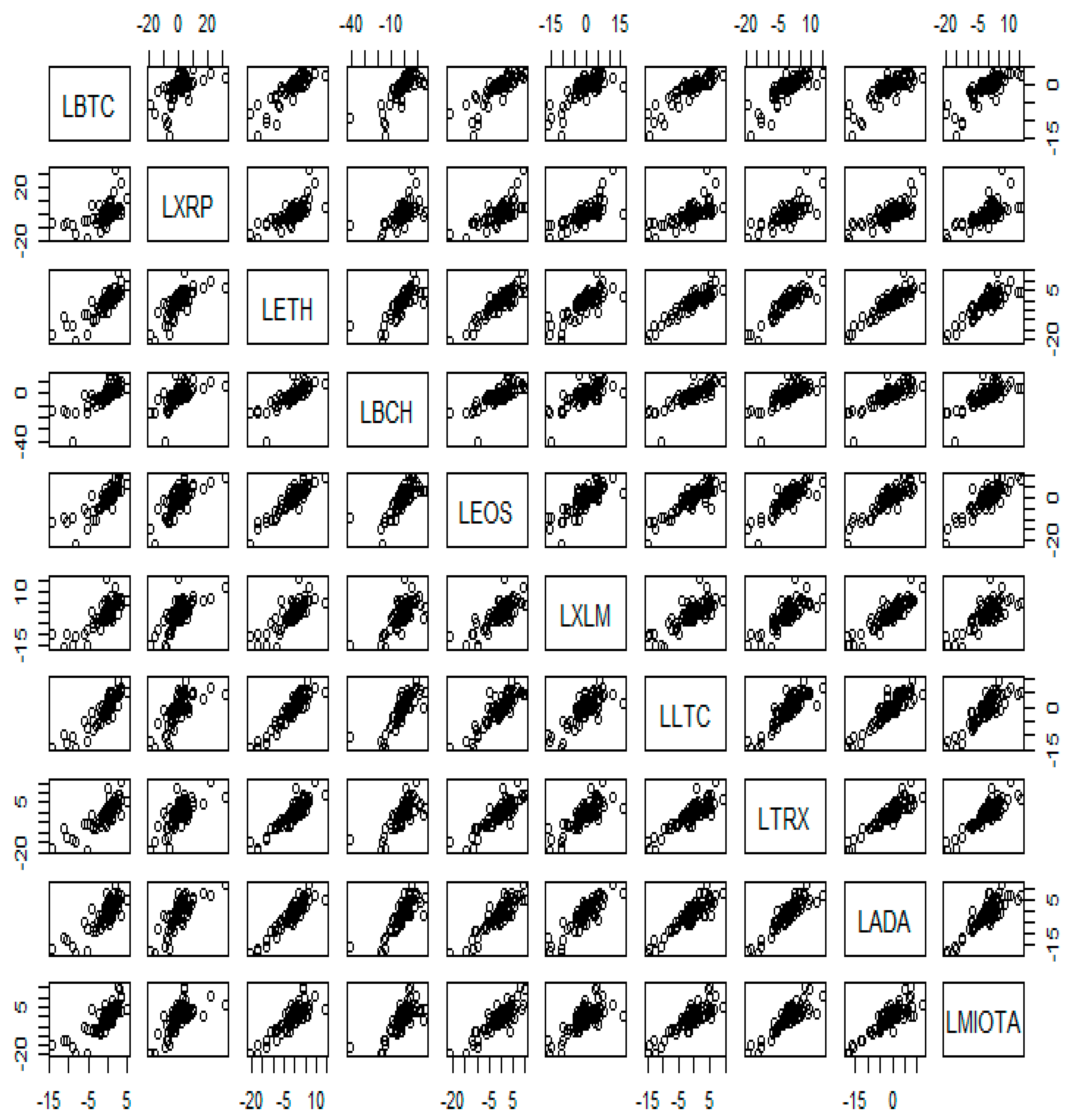
The data set consists of the daily historical prices and volumes of the nine cryptocurrencies. Figure 1 and Figure 2 present the plot of the daily prices of the nine cryptocurrencies. Figure 1 shows the scatterplots among the nine cryptocurrencies from August 2018 to November 2018 (period 1) and Figure 2 from January 2018 to November 2018 (period 2). According to the figures, each pair of cryptocurrencies studied addresses similar results, positive and relatively high correlation regardless of period. For the nine time series data analyses in this section, daily log-returns in percentage are defined as $r_t=100\left[\ln \left(p_t\right)-\ln \left(p_{t-1}\right)\right]$.

Table 1. Descriptive statistics of nine cryptocurrencies.

Period 1
	LBTC	LXRP	LETH	LBCH	LXLM	LLTC	LTRX	LADA	LMIOTA
Minimum	−14.36	−18.80	−20.69	−40.97	−16.14	−14.72	−19.18	−18.41	−19.88
Q1	−0.82	−2.26	−1.82	−3.15	−2.32	−1.84	−2.35	−2.65	−2.31
Median	−0.02	−0.21	−0.39	−0.34	−0.40	−0.43	−0.38	−0.57	−0.06
Mean	−0.51	0.10	−0.98	−1.12	−0.44	−0.61	−0.59	−1.00	−0.61
Q3	0.74	1.79	1.38	1.47	2.21	1.38	1.86	1.66	2.13
Maximum	4.74	32.20	14.22	15.87	16.27	9.28	15.21	11.90	15.87
Skewness	−2.25	1.30	−1.16	−1.89	−0.46	−1.00	−0.56	−0.96	−0.74
Kurtosis	9.70	10.19	6.40	13.50	5.22	4.94	5.24	5.03	5.57
Period 2
	LBTC	LXRP	LETH	LBCH	LXLM	LLTC	LTRX	LADA	LMIOTA
Minimum	−18.46	−35.33	−20.69	−40.97	−30.62	−21.19	−32.87	−21.73	−29.15
Q1	−2.02	−3.88	−2.98	−4.20	−3.69	−3.41	−4.47	−4.34	−4.75
Median	0.08	−0.52	−0.30	−0.50	−0.49	−0.46	−0.71	−1.03	−0.56
Mean	−0.39	−0.57	−0.59	−0.79	−0.36	−0.61	−0.45	−0.91	−0.81
Q3	1.45	2.22	2.21	2.20	3.41	2.42	2.84	2.51	3.58
Maximum	12.41	32.20	14.22	29.34	46.18	29.06	78.67	32.21	22.50
Skewness	−0.59	−0.01	−0.46	−0.55	0.56	0.28	2.00	0.53	−0.32
Kurtosis	5.32	8.00	4.46	7.97	9.30	6.38	18.96	5.84	4.07

Note: The first quartile, Q1, is the 25th percentile and the third quartile, Q3, is the 75th percentile.

shows the summary statistics of the log returns of the nine cryptocurrencies. In general, they share the fat-tail distribution, one of the common characteristics found in the return series of financial assets. Based on the kurtosis statistics, the fat-tailed distribution is observed in all nine cryptocurrencies, though the degree of the fat-tail is quite different among them. One of the interesting observations is the change in kurtosis values between periods 1 and 2. In period 1, the values of the kurtosis of major cryptocurrencies, BTC, XRP, ETH, and BCH (the top 4 based on market capitalization), are higher than the other relatively small market-cap cryptocurrencies (XLM, LTC, TRX, ADA, and MIOTA). This phenomenon is reversed in period 2 where the small-cap cryptocurrencies generally have higher kurtosis values than the large-cap ones. It suggests that over the period of 2018 (period 1), small-cap cryptocurrencies tend to have more extreme daily returns on both directions which can be identified by the magnitude of their minimum and maximum returns in each period. When we focus on the recent data of period 1, however, this trend is reversed. The large-cap cryptocurrencies show higher kurtosis. As for the skewness, all the cryptocurrencies except XRP show lower skewness in the more recent period (period 1) while XRP displays even higher positive skewness. This is an interesting observation because most financial asset returns show a negative skewness. Only XRP has tended to the positively-skewed return series from the negatively-skewed ones while other cryptocurrencies have enhanced the magnitude of skewness in a negative direction. This might be explained by the fact that the most recent bull market period in the crypto market, late 2017 to early 2018, is covered in the data period, and the positive returns during the period dominate the negative returns before and after the bull market in terms of the magnitude. XRP, however, is off this trend. It has been observed that in the more recent period (period 2), a bear market, XRP is the only one which tends to have more extreme positive returns. This implies that the co- movement of XRP with the cryptocurrency market is lower than any other cryptocurrencies and thus its systematic risk in the cryptocurrency market would be low. It might, therefore, attract more attention from potential investors looking to build a market-portfolio in the cryptocurrency market.

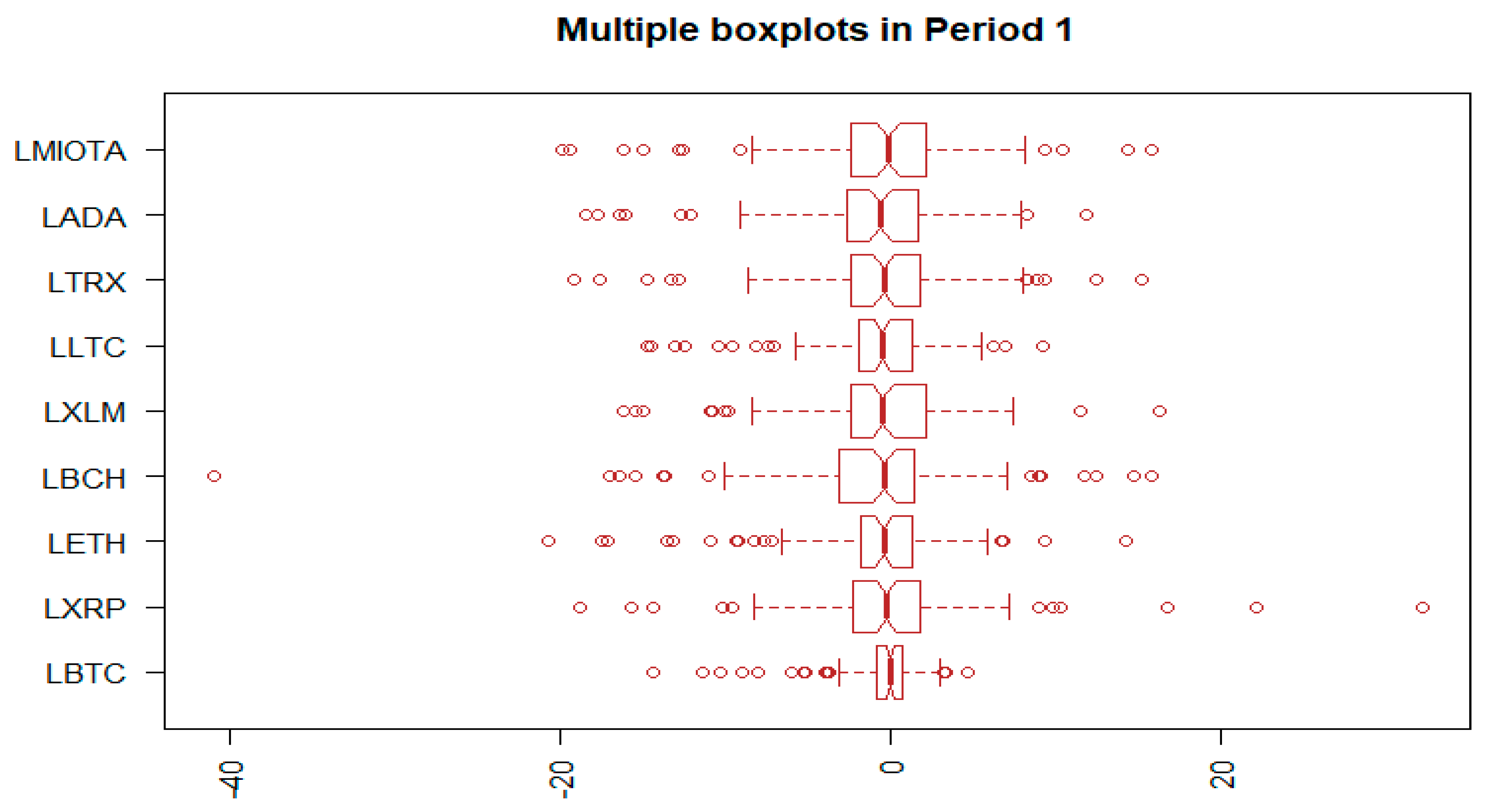
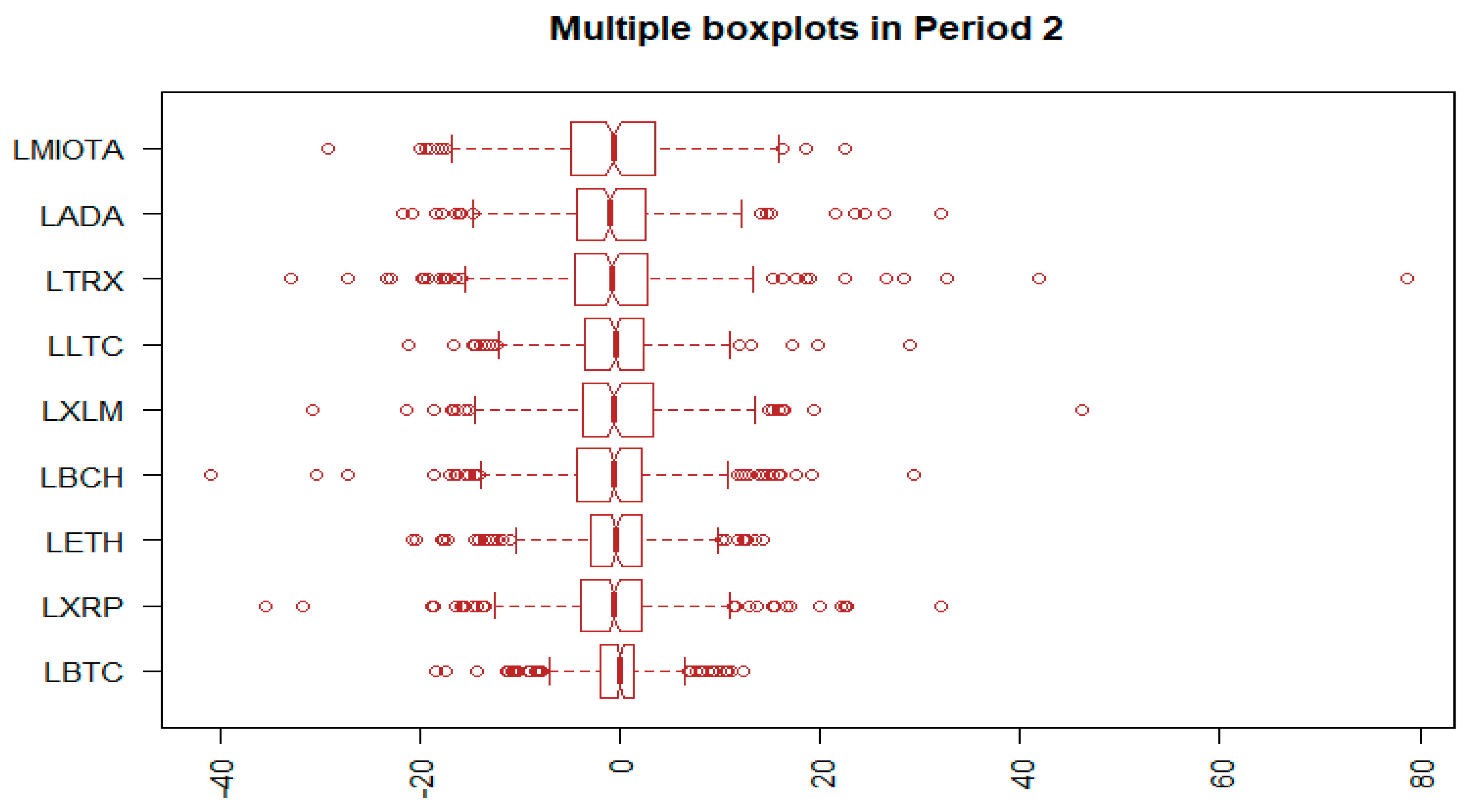
Figure 3 and Figure 4 support the arguments by addressing boxplots of the cryptocurrencies in each period. All cryptocurrencies tend to have extreme log returns on both sides (high kurtosis) and in Figure 3, XRP shows the positively-skewed distribution in the more recent period (period 1). Panels A and B in

Table 2. Pearson’s and Kendall’s Correlations of the nine cryptocurrencies for Period 1.

Panel A: Pearson’s Correlations for Period 1
	LBTC	LXRP	LETH	LBCH	LEOS	LXLM	LLTC	LTRX	LADA	LMIOTA
LBTC	1	0.54	0.84	0.75	0.82	0.75	0.87	0.79	0.81	0.79
LXRP	0.54	1	0.73	0.57	0.7	0.71	0.67	0.7	0.76	0.67
LETH	0.84	0.73	1	0.78	0.91	0.78	0.91	0.89	0.91	0.84
LBCH	0.75	0.57	0.78	1	0.75	0.69	0.8	0.73	0.8	0.73
LEOS	0.82	0.7	0.91	0.75	1	0.77	0.87	0.85	0.89	0.86
LXLM	0.75	0.71	0.78	0.69	0.77	1	0.78	0.78	0.87	0.74
LLTC	0.87	0.67	0.91	0.8	0.87	0.78	1	0.87	0.9	0.86
LTRX	0.79	0.7	0.89	0.73	0.85	0.78	0.87	1	0.9	0.87
LADA	0.81	0.76	0.91	0.8	0.89	0.87	0.9	0.9	1	0.86
LMIOTA	0.79	0.67	0.84	0.73	0.86	0.74	0.86	0.87	0.86	1
Panel B: Kendall’s Correlations for Period 1
	LBTC	LXRP	LETH	LBCH	LEOS	LXLM	LLTC	LTRX	LADA	LMIOTA
LBTC	1	0.45	0.65	0.62	0.61	0.46	0.66	0.58	0.57	0.54
LXRP	0.45	1	0.6	0.44	0.5	0.52	0.52	0.47	0.57	0.51
LETH	0.65	0.6	1	0.65	0.66	0.58	0.7	0.66	0.69	0.57
LBCH	0.62	0.44	0.65	1	0.63	0.49	0.65	0.57	0.6	0.55
LEOS	0.61	0.5	0.66	0.63	1	0.52	0.65	0.61	0.65	0.58
LXLM	0.46	0.52	0.58	0.49	0.52	1	0.54	0.52	0.64	0.47
LLTC	0.66	0.52	0.7	0.65	0.65	0.54	1	0.63	0.66	0.6
LTRX	0.58	0.47	0.66	0.57	0.61	0.52	0.63	1	0.67	0.6
LADA	0.57	0.57	0.69	0.6	0.65	0.64	0.66	0.67	1	0.59
LMIOTA	0.54	0.51	0.57	0.55	0.58	0.47	0.6	0.6	0.59	1

and

Table 3. Pearson’s and Kendall’s Correlations of nine cryptocurrencies for Period 2.

Panel A: Pearson’s Correlations for Period 2
	LBTC	LXRP	LETH	LBCH	LEOS	LXLM	LLTC	LTRX	LADA	LMIOTA
LBTC	1	0.68	0.81	0.8	0.69	0.68	0.84	0.63	0.74	0.76
LXRP	0.68	1	0.74	0.66	0.68	0.74	0.71	0.63	0.78	0.73
LETH	0.81	0.74	1	0.79	0.71	0.71	0.83	0.61	0.79	0.8
LBCH	0.8	0.66	0.79	1	0.68	0.64	0.8	0.56	0.7	0.76
LEOS	0.69	0.68	0.71	0.68	1	0.63	0.7	0.58	0.73	0.67
LXLM	0.68	0.74	0.71	0.64	0.63	1	0.66	0.5	0.83	0.68
LLTC	0.84	0.71	0.83	0.8	0.7	0.66	1	0.56	0.73	0.78
LTRX	0.63	0.63	0.61	0.56	0.58	0.5	0.56	1	0.6	0.58
LADA	0.74	0.78	0.79	0.7	0.73	0.83	0.73	0.6	1	0.76
LMIOTA	0.76	0.73	0.8	0.76	0.67	0.68	0.78	0.58	0.76	1
Panel B: Kendall’s Correlations for Period 2
	LBTC	LXRP	LETH	LBCH	LEOS	LXLM	LLTC	LTRX	LADA	LMIOTA
LBTC	1	0.55	0.65	0.65	0.55	0.54	0.67	0.55	0.59	0.56
LXRP	0.55	1	0.66	0.57	0.56	0.6	0.6	0.55	0.63	0.58
LETH	0.65	0.66	1	0.68	0.61	0.57	0.69	0.57	0.66	0.61
LBCH	0.65	0.57	0.68	1	0.57	0.53	0.69	0.55	0.59	0.59
LEOS	0.55	0.56	0.61	0.57	1	0.54	0.58	0.55	0.59	0.54
LXLM	0.54	0.6	0.57	0.53	0.54	1	0.54	0.51	0.66	0.52
LLTC	0.67	0.6	0.69	0.69	0.58	0.54	1	0.54	0.61	0.6
LTRX	0.55	0.55	0.57	0.55	0.55	0.51	0.54	1	0.56	0.53
LADA	0.59	0.63	0.66	0.59	0.59	0.66	0.61	0.56	1	0.58
LMIOTA	0.56	0.58	0.61	0.59	0.54	0.52	0.6	0.53	0.58	1

show the correlations of the nine cryptocurrencies for each period. We report both Pearson’s and Kendall’s correlation coefficients. Based on the Pearson’s correlation matrix, the magnitude of correlation coefficients tends to be higher toward to the recent period (from period 1 to 2) except in several pairs, especially XRP-related pairs (BTC-XRP from 0.68 to 0.54), which show lower magnitudes.

When we look into the results of the Kendall’s coefficients; however, the trends addressed in the Pearson’s results [33] show the opposite directions. Most correlation pairs in the Kendall’s coefficient table were lower from period 1 to 2 (the recent period). However, with regard to the seemingly contradictory direction between the two types of correlation coefficients we suggest that Kendall’s reflects the skewed and fat-tailed distribution feature of the return data of cryptocurrencies. Kendall’s correlation coefficients are the rank correlation, a non-parametric test that measures the strength of dependence between two variables, whereas Pearson’s are calculated based on the normality assumption. Principal component analysis (hereafter, PCA) is an effective multivariate statistical analysis technique for reducing the dimension of large data sets with minimal loss of information and extracting their structural features ([2]). It transforms a number of correlated variables into a series of linearly uncorrelated variables called principal components by projecting the observation results onto axes to capture the maximum amount of variability in the original data. The first principal component explains the largest possible variability of the original data, and each succeeding component in turn explains the highest variability under the constraint that it is orthogonal to the preceding components. PCA is optimal from the perspective of minimizing the square distance between the observed values in the input space and the mapped values in the low-dimensional subspace ([12]).

Table 4. Principal Component Analysis Results for Period 1 and Period 2.

Period 1
	PC1	PC2	PC3	PC4	PC5	PC6	PC7	PC8	PC9
Standard deviation	2.70	0.73	0.55	0.52	0.45	0.39	0.32	0.27	0.24
Proportion of Variance	0.81	0.06	0.03	0.03	0.02	0.02	0.01	0.01	0.01
Cumulative Proportion	0.81	0.87	0.90	0.93	0.96	0.97	0.99	0.99	1.00
Period 2
	PC1	PC2	PC3	PC4	PC5	PC6	PC7	PC8	PC9
Standard deviation	2.59	0.75	0.74	0.53	0.48	0.47	0.42	0.37	0.37
Proportion of Variance	0.75	0.06	0.06	0.03	0.03	0.02	0.02	0.02	0.01
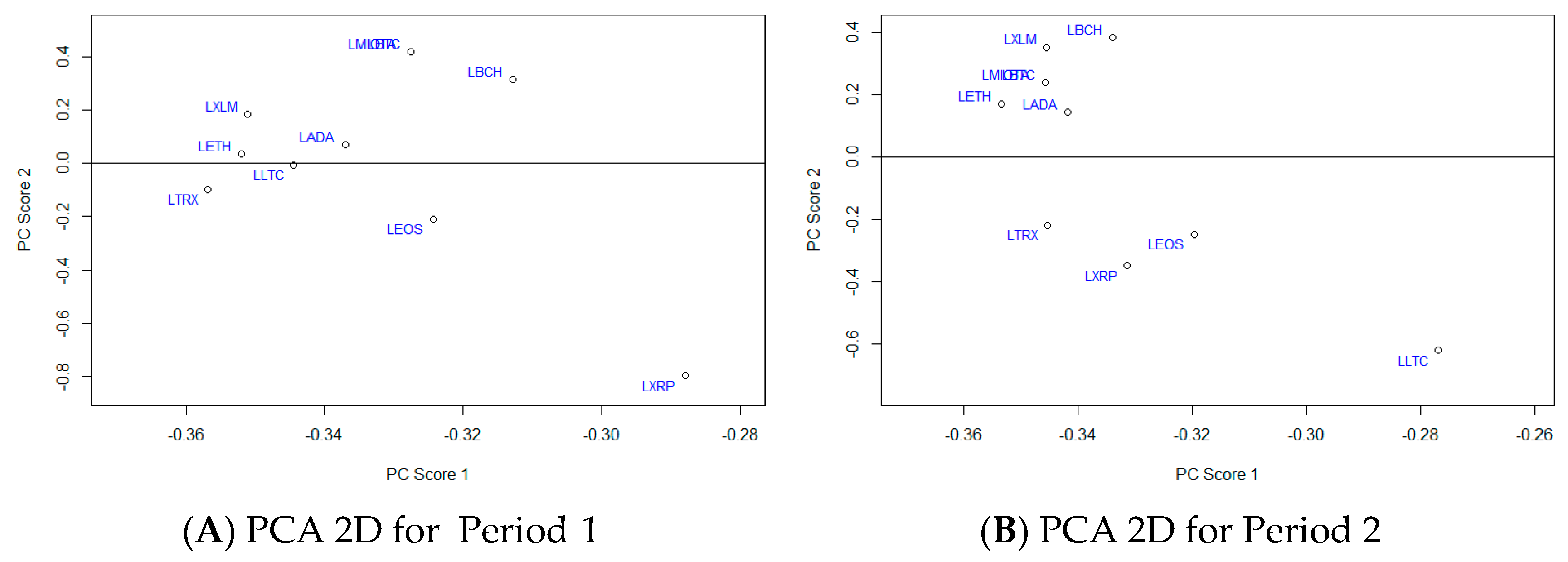
Cumulative Proportion	0.75	0.81	0.87	0.90	0.93	0.95	0.97	0.99	1.00

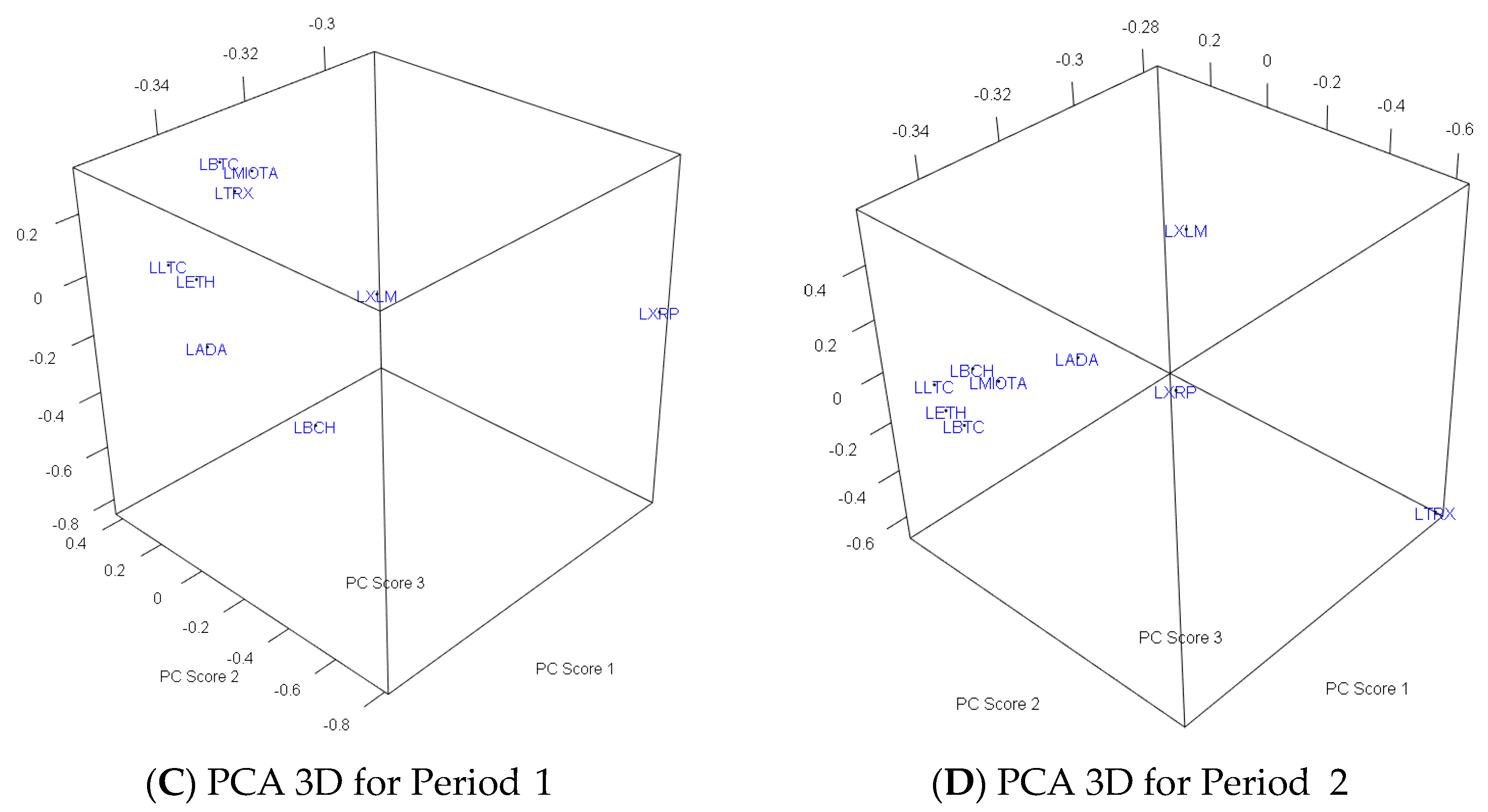
shows the PCA [34] results for periods 1 and 2. The proportion of variance explained by the first principal component in period 1 is 81% whereas it is 75% in period 2. Figure 5 addresses the factor loadings of the first two main components in panels A and Band the three main components (panels C and D). ETH, TRX, and XLM are the variables with high magnitude (an absolute term) of factor loadings in the first component in both periods. Interestingly, the signs of the factor scores are positive across all factors in period 1. In the second component, BCH, XLM, and BTC, has factor loadings that are influential on both periods. In period 1, the XRP return series shows the largest factor loading in an absolute term, around −0.8, in the second component, whereas LTC does the same in period 2.

Table 5. The GARCH model comparison by AIC.

Period 1
Model	LBTC	LXRP	LETH	LBCH	LXLM	LLTC	LTRX	LADA	LMIOTA
GARCH	4.8739	6.6063	6.1915	6.7408	6.0758	5.837	6.2866	6.2496	6.3921
TGARCH	4.2663	6.1826	5.7409	6.2895	5.9421	5.6703	6.0792	6.0508	6.101
IGARCH	4.2092	6.1941	5.701	6.233	5.9543	5.6255	6.0474	6.0125	6.0705
Period 2
Model	LBTC	LXRP	LETH	LBCH	LXLM	LLTC	LTRX	LADA	LMIOTA
GARCH	5.5575	6.5704	6.2413	6.7238	6.6179	6.1644	6.9547	6.6813	6.7404
TGARCH	5.3532	6.4055	6.1472	6.5719	6.5485	6.1061	6.8471	6.5956	6.6676
IGARCH	5.3331	6.381	6.1285	6.5465	6.5255	6.0937	6.8272	6.5809	6.6673

shows the value of the AIC (Akaike’s information criterion) of different GARCH models (GARCH, TGARCH, and IGARCH) across nine cryptocurrencies in each period. We include TGARCH to handle the asymmetric distribution of errors which is commonly known for cryptocurrencies ([30]). In period 1, the IGARCH model provides the lowest AIC except for XRP, BCH, and LTC where the TGARCH models have the lowest AIC. In period 2, however, IGARCH shows the lowest AIC over all of cryptocurrencies. Given the value of the AIC model selection criterion, this indicates that in general IGARCH is superior to other GARCH family models.

Table 6. IGARCH with ARMA(0,0) with LBTC for Period 1 and Period 2.

	IGARCH (1,1)
	Period 1			Period 2
	Coefficient	Std. Error	p-Value	Coefficient	Std. Error	p-Value
Μ	0.02596	0.11163	0.81608	−0.03004	0.11346	0.76067
${\alpha }_0$	0.06939	0.14897	0.64139	0.00018	0.05485	0.99738
${\alpha }_1$	0.10835	0.0649	0.09504	0.06961	0.02047	0.00067
${\beta }_1$	0.89165	NA	NA	0.9304	NA	NA
Shape	2.619532	0.24391	0.00000	3.57618	0.38593	0.00000
Log likelihood	−208.5649			−875.9657
N	101			330
AIC	4.2092			5.3331

Note: The return equation is: $r_t=\mu +{\epsilon }_t.$ The variance equation is $a_t=\sqrt{h_t}{e}_t$ and $h_t={\alpha }_0+{\alpha }_1{a}_{t-1}^2+{\beta }_1{h}_{t-1}$ where ${\alpha }_0>0,{\alpha }_i\ge 0,{\beta }_i\ge 0,{\alpha }_1+{\beta }_1=1\left({\beta }_1=1-{\alpha }_1\right)$ and $e_t$~t-Student distribution with shape parameter.

shows the reliability of the IGARCH with ARMA (0,0) with LBTC for Period 1 and Period 2 even though ${\alpha }_1$ is statistically significant at the significance level (0.10) for Period 1.

Table 7. Volatility prediction performance of the SV and GARCH models ¹.

	LBTC				LXRP				LETH
Forecasting Horizons	Period 1		Period 2		Period 1		Period 2		Period 1		Period 2
MSE1	IGARCH	SV	IGARCH	SV	TGARCH	SV	IGARCH	SV	IGARCH	SV	IGARCH	SV
h = 44	9.198	5.761	8.228	5.946	7.492	4.468	15.385	5.424	5.669	5.625	10.225	6.155
h = 30	6.479	5.067	5.767	4.253	6.144	3.628	11.501	4.371	5.030	4.987	8.124	5.251
h = 20	6.782	4.976	6.074	4.519	5.704	2.958	10.065	3.798	3.991	3.881	8.096	4.621
h = 10	3.973	5.127	3.580	3.047	3.269	1.781	5.035	2.112	2.421	2.341	3.660	2.217
h = 5	6.219	5.738	5.731	4.959	2.891	1.460	4.049	1.788	1.535	1.365	2.393	1.199
h = 3	8.485	8.165	8.038	7.407	0.989	1.116	1.329	0.819	2.010	1.729	1.230	0.995
MSE2	IGARCH	SV	IGARCH	SV	TGARCH	SV	IGARCH	SV	IGARCH	SV	IGARCH	SV
h = 44	8.928	1.293	7.569	4.080	9.069	3.976	19.382	5.776	2.932	2.831	11.999	4.880
h = 30	7.525	0.989	6.344	3.399	8.270	3.469	15.902	5.147	2.524	2.445	10.327	4.355
h = 20	7.642	1.000	6.500	3.729	8.301	3.430	14.183	5.129	2.653	2.570	10.531	4.699
h = 10	5.832	0.826	4.883	2.960	6.488	2.380	9.507	3.745	1.419	1.459	7.419	3.108
h = 5	6.788	1.154	5.810	4.011	6.154	2.241	7.938	3.537	1.129	1.193	6.669	2.795
h = 3	7.202	1.784	6.252	4.658	4.209	1.207	5.185	2.102	0.683	0.776	5.299	2.036

¹ This table shows the performance of the volatility prediction using the daily log-returns over the period (28 November 2018 to 10 January 2019) of Bitcoin (BTC), XRP (XRP), and Ethereum (ETH) which are denoted by LBTC, LXRP, and LETH, respectively, with training data (periods 1 and 2).

,

Table 8. Volatility prediction performance of the SV and GARCH models ¹.

	LBCH				LXML				LLTC
Forecasting Horizons	Period 1		Period 2		Period 1		Period 2		Period 1		Period 2
MSE1	TGARCH	SV	IGARCH	SV	TGARCH	SV	IGARCH	SV	IGARCH	SV	IGARCH	SV
h = 44	11.408	11.373	15.203	12.152	7.671	5.557	10.698	6.924	3.859	3.247	4.223	3.264
h = 30	13.736	13.693	17.193	14.353	5.851	4.454	7.796	5.255	4.384	3.380	4.663	3.591
h = 20	12.554	12.433	16.338	13.276	3.597	2.606	4.893	3.060	4.043	3.079	4.039	3.188
h = 10	21.747	21.510	27.494	23.089	2.818	2.156	3.426	2.286	4.471	3.798	4.135	3.641
h = 5	37.270	36.627	49.146	40.633	2.707	1.433	3.222	1.936	2.493	1.769	2.063	1.666
h = 3	0.135	0.959	1.112	0.148	3.690	2.346	4.067	2.876	1.929	1.811	1.576	1.479
MSE2	TGARCH	SV	IGARCH	SV	TGARCH	SV	IGARCH	SV	IGARCH	SV	IGARCH	SV
h = 44	5.171	5.025	12.692	7.230	8.318	3.811	12.786	6.900	5.424	1.779	6.317	3.580
h = 30	5.677	5.462	12.948	7.612	7.309	3.087	10.744	5.902	6.058	1.979	6.506	3.883
h = 20	5.613	5.250	12.963	7.530	6.494	2.356	9.142	5.022	6.171	1.816	6.033	3.683
h = 10	8.941	8.194	17.094	10.910	6.266	2.035	7.865	4.550	6.501	1.803	5.484	3.572
h = 5	15.764	14.319	26.754	18.301	7.027	2.240	8.011	4.946	6.322	1.329	4.727	3.068
h = 3	1.677	0.571	7.042	2.189	7.478	2.543	8.092	5.242	5.864	1.125	4.050	2.686

¹ This table shows the performance of the volatility prediction using the daily log-returns over the period (28 November 2018 to 10 January 2019) of Bitcoin Cash (BCH), Stellar (XLM), and Litecoin (LTC) which are denoted by LBCH, LXLM, and LLTC, respectively, with training data (periods 1 and 2).

and

Table 9. Volatility prediction performance of the SV and GARCH models ¹.

	LTRX				LADA				LMIOTA
Forecasting Horizons	Period 1		Period 2		Period 1		Period 2		Period 1		Period 2
MSE1	IGARCH	SV	IGARCH	SV	IGARCH	SV	IGARCH	SV	IGARCH	SV	IGARCH	SV
h = 44	16.159	6.082	9.827	7.943	9.422	3.953	6.049	4.688	16.957	8.462	12.658	9.737
h = 30	16.762	7.006	11.074	9.239	9.446	4.509	6.744	5.406	17.327	10.830	14.268	11.891
h = 20	17.646	7.727	12.330	10.444	9.058	4.706	7.007	5.700	8.469	4.833	6.904	5.311
h = 10	3.379	2.465	2.151	1.928	8.040	5.904	7.345	6.417	9.816	5.502	8.700	6.706
h = 5	3.563	3.970	2.825	2.941	13.804	9.954	13.054	11.433	3.998	2.208	3.806	2.513
h = 3	1.894	5.587	1.759	2.798	12.428	10.271	12.213	11.091	2.567	2.735	2.660	2.084
MSE2	IGARCH	SV	IGARCH	SV	IGARCH	SV	IGARCH	SV	IGARCH	SV	IGARCH	SV
h = 44	19.763	3.760	11.030	7.828	14.335	3.158	8.669	5.747	18.503	3.887	12.473	7.478
h = 30	18.551	4.234	11.245	8.380	13.214	3.470	8.795	6.120	16.598	4.339	12.149	7.800
h = 20	17.746	4.734	11.694	9.012	12.065	3.643	8.800	6.298	12.097	2.492	9.308	5.598
h = 10	7.929	1.292	5.441	3.723	9.620	3.667	8.106	5.894	11.491	3.135	10.186	6.494
h = 5	5.965	1.260	4.818	3.271	11.809	5.863	10.958	8.419	7.827	1.756	7.854	4.508
h = 3	2.750	0.290	2.460	1.337	9.948	5.230	9.684	7.385	5.860	1.256	6.455	3.406

¹ This table shows the performance of the volatility prediction using the daily log-returns over the period (28 November 2018 to 10 January 2019) of TRON (TRX), Cardano (ADA), and IOTA (IOTA) which are denoted by LTRX, LADA, and LMIOTA, respectively, with the training data (periods 1 and 2).

demonstrate representative results regarding forecast accuracy for an h-step-ahead forecast. We report out-of-sample MSE losses in both the SV and GARCH models with the observed time series data, where the evaluation is based on two different volatility proxies for the conditional volatility. The forecast losses of the models are systematically lower over all horizons and across all cryptocurrencies. The results exhibit the superior forecasting accuracy of the SV method over the GARCH models, especially in volatility forecasting over longer time horizons. For example, 3 day out-of-sample MSEs (Mean Squared Errors) (using the variance as a conditional volatility) of the BTC over period 1 are 8.485 and 8.165 for IGARCH and SV, respectively, and those of period 2 are 8.038 and 7.407, respectively. When the forecasting time horizon is the longest (h = 44), the MSE of the SV method is 5.761 in period 1, whereas that of the IGARCH is 9.198. Thus, the SV method has better forecasting accuracy than the IGARCH as the forecasting horizon is longer.

This trend is shown in all other cryptocurrencies, regardless of the conditional volatility types (MSE1 and MSE2). This difference of MSEs between TGARCH and SV is high in TRX, ADA, and MIOTA while ETH has almost no difference in period 1 (5.669 for the TGARCH and 6.625 for the SV method). In general, the SV method shows better forecasting accuracy than the GARCH models across all the cryptocurrencies, especially in volatility forecasting over longer time horizons. One plausible reason is that the SV model allows for two error processes and thus is more flexible for modeling financial time series, while the GARCH model considers a single error term. In addition to that, the SV model allow us to use the Bayesian approach to determine the inferences for the volatilities of time series using simulation algorithms such as the Markov Chain Monte Carlo (MCMC) methods whereas the GARCH family models have the difficulty of obtaining the maximum likelihood estimates caused by the complexity of the likelihood function. Therefore, the SV model offers a better in-sample fit ([3]).

4. Discussion

During period 1 (low volatile period) and period 2 (high volatile period), our finding is that the SV method shows better forecasting accuracy in terms of volatility. It indicates that institutional investors and individuals adopting cryptocurrency in their investment portfolios may better prepare for future risk management by utilizing SV models. Recently, the prices of cryptocurrency have been decreased by about 50 percent from the highest price in the early of April 2021. Investors are experiencing another round of high volatility time regarding cryptocurrency. The unexpected abrupt change of price of cryptocurrency may not be able to prepare well for the risk management to institutional investors even by employing neural network based volatility models because of the lack of the investment environment information training data about the cryptocurrency. Under this financial situation such that a sudden increase in the volatility of portfolio can bring tremendous risks including an increase in currency hedging costs, an increase in damage to loans for institutions, and a decrease in the value of beneficiary certificates, we can strongly recommend the investors to use the SV method which are confirmed by our finding with the low and high volatility time series data.

5. Conclusions

Understanding the volatility of the most popular cryptocurrencies is important to both investors and policymakers. In this study, we discussed the volatility of nine cryptocurrencies by using the GARCH and SV models. While previous studies have employed a variation of GARCH models, we introduced another statistical method for better out-of- sample forecasting power, the SV model. Our results provide strong empirical evidence that when we deal with extremely volatile financial data, such as cryptocurrencies, the SV method has better forecasting accuracy power than the GARCH models in terms of volatility, and this tendency is stronger as the forecasting horizons are longer. Finally, our SV model sheds light on the significance of a risk management tool for extremely volatile assets such as cryptocurrency. In this study, we only used ten cryptocurrency coins to compare the SV and GARCH models for volatility forecasting. In our future study, we will use more than 30 numbers of cryptocurrency coins to compare the neural network-based volatility model to the SV model with the recent cryptocurrency time series data. For forecasting the price of cryptocurrency, we are going to use a recurrent neural networks and long short-term memory models with traditional time series models such as the autoregressive integrated moving average model and ETS (Error, Trend, Seasonal) models.

References

1. Bacao, P.; Duarte, A.; Sebastiao, H.; Redzepagic, S. Information Transmission between Cryptocurrencies: Does Bitcoin Rule the Cryptocurrency World? Sci. Ann. Econ. Bus. 2018, 65, 97–117. [Google Scholar]
2. Nakamoto, S. Bitcoin: A Peer-to-Peer Electronic Cash System. 2008. Available online: https://bitcoin.org/bitcoin.pdf (accessed on 15 June 2021).
3. Kim, J.-M.; Kim, S.; Kim, S.T. On the Relationship of Cryptocurrency Price with US Stock and Gold Price using Copula Models. Mathematics 2020, 8, 1859. [Google Scholar] [CrossRef]
4. Corbet, S.; Meegan, A.; Larkin, C.; Lucey, B.; Yarovaya, L. Exploring the dynamic relationships between cryptocurrencies and other financial assets. Econ. Lett. 2018, 165, 28–34. [Google Scholar] [CrossRef] [Green Version]
5. Grinberg, R. Bitcoin: An innovative alternative digital currency. Hastings Sci. Technol. Law J. 2011, 4, 160–207. [Google Scholar]
6. Dyhrberg, A.H. Bitcoin, gold and the dollar-A GARCH volatility analysis. Financ. Res. Lett. 2015, 16, 85–92. [Google Scholar] [CrossRef] [Green Version]
7. Hencic, A.; Gourieroux, C. Noncausal Autoregressive Model in Application to Bitcoin/USD Exchange Rate. In Proceedings of the 7th Financial Risks International Forum, Paris, France, 20–21 March 2014; pp. 1–25. [Google Scholar]
8. Dwyer, G.P. The economics of Bitcoin and similar private digital currencies. J. Financ. Stab. 2015, 17, 81–91. [Google Scholar] [CrossRef] [Green Version]
9. Bariviera, A.F. The inefficiency of Bitcoin revisited: A dynamic approach. Econ. Lett. 2017, 161, 1–4. [Google Scholar] [CrossRef] [Green Version]
10. Gkillas, K.; Katsiampa, P. An Application of Extreme Value Theory to Cryptocurrencies. Econ. Lett. 2018, 164, 109–111. [Google Scholar] [CrossRef] [Green Version]
11. Hansen, P.R.; Lunde, A. A Forecast Comparison of Volatility Models: Does Anything Beat a GARCH(1, 1)? J. Appl. Econom. 2005, 20, 873–889. [Google Scholar] [CrossRef] [Green Version]
12. Hyndman, R.; Athanasopoulos, G.; Bergmeir, C.; Caceres, G.; Chhay, L.; O’Hara- Wild, M.; Petropoulos, F.; Razbash, S.; Wang, E. Forecast: Forecasting Functions for Time Series and Linear Models; R Foundation Package: Vienna, Austria, 2018. [Google Scholar]
13. Katsiampa, P. Volatility estimation for Bitcoin: A comparison of GARCH models. Econ. Lett. 2017, 158, 3–6. [Google Scholar] [CrossRef] [Green Version]
14. Katsiampa, P. An empirical investigation of volatility dynamics in the cryptocurrency market. Res. Int. Bus. Financ. 2019, 50, 322–335. [Google Scholar] [CrossRef]
15. Caporale, G.M.; Zekokh, T. Modelling volatility of cryptocurrencies using Markov-Switching models. Res. Int. Bus. Financ. 2019, 48, 143–155. [Google Scholar] [CrossRef]
16. Klein, T.; Thu, H.P.; Walther, T. Bitcoin is not the New Gold—A comparison of volatility, correlation, and portfolio performance. Int. Rev. Financ. Anal. 2018, 59, 105–116. [Google Scholar] [CrossRef]
17. Phillip, A.; Chan, J.S.; Peiris, S. A new look at Cryptocurrencies. Econ. Lett. 2018, 163, 6–9. [Google Scholar] [CrossRef]
18. Phillip, A.; Chan, J.; Peiris, S. On long memory effects in the volatility measure of Cryptocurrencies. Financ. Res. Lett. 2019, 28, 95–100. [Google Scholar] [CrossRef]
19. Hyun, S.; Lee, J.M.; Kim, J.M.; Jun, C. What coins lead in the cryptocurrency market? Using Copula and Neural Network Models. J. Risk Financial Manag. 2019, 12, 132. [Google Scholar] [CrossRef] [Green Version]
20. Bollerslev, T. Generalized Autoregressive Conditional Heteroskedasticity. J. Econom. 1986, 31, 307–327. [Google Scholar] [CrossRef] [Green Version]
21. Engle, R.F. Autoregressive Conditional Heteroscedasticity with Estimates of the Variance of United Kingdom Inflation. Econometrica 1982, 50, 987–1007. [Google Scholar] [CrossRef]
22. Black, F. The pricing of commodity contracts. J. Financ. Econ. 1976, 3, 167–179. [Google Scholar] [CrossRef]
23. Kim, J.M.; Jung, H.; Qin, L. New Generalized Volatility Proxy via Stochastic Volatility Model. Appl. Econ. 2017, 49, 2259–2268. [Google Scholar] [CrossRef]
24. Ghalanos, A. The Rmgarch Models: Background and Properties, Version 1.2-8. 2015. Available online: https://cran.r-project.org/ (accessed on 15 June 2021).
25. Engle, R.F.; Bollerslev, T. Modeling the persistence of conditional variances. Econom. Rev. 1986, 5, 1–50. [Google Scholar] [CrossRef]
26. Zakoian, J.M. Threshold heteroskedastic models. J. Econ. Dyn. Control 1994, 18, 931–955. [Google Scholar] [CrossRef]
27. Kim, J.-M.; Hwang, S.Y. The Copula Directional Dependence by Stochastic Volatility Models. Commun. Stat. Simul. Comput. 2019, 48, 1153–1175. [Google Scholar] [CrossRef]
28. Kim, J.-M.; Jung, H. Time Series Forecasting using Functional Partial Least Square Regression with Stochastic Volatility, GARCH and Exponential Smoothing. J. Forecast. 2018, 37, 269–280. [Google Scholar] [CrossRef]
29. Kim, S.; Shephard, N.; Chib, S. Stochastic Volatility: Likelihood Inference and Comparison with ARCH Models. Rev. Econ. Stud. 1998, 65, 361–393. [Google Scholar] [CrossRef]
30. Taylor, S.J. Financial returns modelled by the product of two stochastic processes-a study of the daily sugar prices 1961–1975. Time Ser. Anal. Theory Pract. 1982, 1, 203–226. [Google Scholar]
31. Kastner, G. Dealing with Stochastic Volatility in Time Series Using the R Package ‘stochvol’. J. Stat. Softw. 2016, 69. [Google Scholar] [CrossRef] [Green Version]
32. Hentschel, L. All in the Family Nesting Symmetric and Asymmetric GARCH Models. J. Financ. Econ. 1995, 39, 71–104. [Google Scholar] [CrossRef]
33. Pearson, K. On lines and planes of closest fit to system of points on space. Philos. Mag. 1901, 6, 559–572. [Google Scholar] [CrossRef] [Green Version]
34. Kazor, K.; Holloway, R.W.; Cath, T.Y.; Hering, A.S. Comparison of linear and nonlinear dimension reduction techniques for automated process monitoring of a decentralized waste water treatment facility. Stoch. Environ. Res. Risk Assess. 2016, 30, 1–18. [Google Scholar] [CrossRef]
Figure 1. Scatterplots of the nine cryptocurrencies in period 1 (19 August 2018 to 27 November 2018).
Mathematics 09 01614 g001
Figure 2. Scatterplots of the nine cryptocurrencies in period 2 (2 January 2018 to 27 November 2018).
Mathematics 09 01614 g002
Figure 3. Boxplots of the nine cryptocurrencies in period 1 (19 August 2018 to 27 November 2018).
Mathematics 09 01614 g003
Figure 4. Boxplots of the nine cryptocurrencies in period 2 (2 January 2018 to 27 November 2018).
Mathematics 09 01614 g004
Figure 5. PCA Figures.
Mathematics 09 01614 g005aMathematics 09 01614 g005b