Towards Personalized Diagnosis of Glioblastoma in Fluid-Attenuated Inversion Recovery (FLAIR) by Topological Interpretable Machine Learning

Abstract

Glioblastoma multiforme (GBM) is a fast-growing and highly invasive brain tumor, which tends to occur in adults between the ages of 45 and 70 and it accounts for 52 percent of all primary brain tumors. Usually, GBMs are detected by magnetic resonance images (MRI). Among MRI, a fluid-attenuated inversion recovery (FLAIR) sequence produces high quality digital tumor representation. Fast computer-aided detection and segmentation techniques are needed for overcoming subjective medical doctors (MDs) judgment. This study has three main novelties for demonstrating the role of topological features as new set of radiomics features which can be used as pillars of a personalized diagnostic systems of GBM analysis from FLAIR. For the first time topological data analysis is used for analyzing GBM from three complementary perspectives—tumor growth at cell level, temporal evolution of GBM in follow-up period and eventually GBM detection. The second novelty is represented by the definition of a new Shannon-like topological entropy, the so-called Generator Entropy. The third novelty is the combination of topological and textural features for training automatic interpretable machine learning. These novelties are demonstrated by three numerical experiments. Topological Data Analysis of a simplified 2D tumor growth mathematical model had allowed to understand the bio-chemical conditions that facilitate tumor growth—the higher the concentration of chemical nutrients the more virulent the process. Topological data analysis was used for evaluating GBM temporal progression on FLAIR recorded within 90 days following treatment completion and at progression. The experiment had confirmed that persistent entropy is a viable statistics for monitoring GBM evolution during the follow-up period. In the third experiment we developed a novel methodology based on topological and textural features and automatic interpretable machine learning for automatic GBM classification on FLAIR. The algorithm reached a classification accuracy up to 97%.

1. Introduction

Gliomas are the most common primary brain tumors, originating from glial cells. We can differentiate between benign tumors, with, in some cases, a long life expectancy, and malignant forms. In this second group, glioblastoma multiforme (GBM) is the most frequent malignant cancer with the worst prognosis, with less than 5% of affected patients with a 5-year survival rate and with the highest relapse rate [1]. GBM are characterized by a diffuse and infiltrative growth pattern, as invasive glioma cells often migrate along myelinated white matter (WM) fiber tracts. This is a major cause of their appalling prognosis—tumor cells invade, displace, and possibly destroy WM. For these reasons, surgical, radiotherapic and chemotherapic approaches, also early performed, rarely resulted in being effective for a significant number of months [2]. Moreover, large surgical resections could cause unacceptable effects on motor or speech functions. In largely infiltrative GBM, the real objective of the surgical approach is to leave less possible cancer cells in situ to give more chances to adjuvant therapy. The non-invasive detection of microscopic infiltration, as well as the identification of aggressive tumor components within spatially heterogeneous lesions, are of outstanding importance for surgical and radiation therapy planning or to assess response to chemotherapy. Moreover, the critical importance of an accurate detection of local infiltration is underlined by the results of intraoperative MR—this technique seems to be able to contribute significantly to optimal resection [3] and to improve post-operative outcomes [4]. Magnetic resonance (MR) imaging plays an important role in the detection and evaluation of brain tumors. The evaluation of post-surgical residual cancer by MR should be performed in all patients after 48–72 h after surgery, because this factor has a relevant prognostic value both for survival and for the subsequent therapeutic response [5]. For more than 30 years [6] conventional MR imaging, typically T1w images before and after paramagnetic contrast administration, T2w images and FLAIR images have been largely used to evaluate brain neoplasms. MR allows to localize the lesions, helps to distinguish tumors from other pathological processes, and depicts basic signs of response to therapy, such as changes in size and degree of contrast enhancement. Manual tumor detection and segmentation on MR images is time-consuming and can have a great inter-observer variability; automatic segmentation is more reproducible and efficient when robustness is particularly desirable, such as in monitoring disease progression or in the longitudinal evaluation of emerging therapies [7]. This is a very relevant element because often in clinical practice the decisions regarding therapy continuation or discontinuation are taken on the basis of disease recovery [2]. Radiomics is a set of techniques for extracting a vectorial representation that provides a quantitative description of tumor radiographic data. In general, radiomics extracts quantitative description of signals and images intensity, texture description and geometric characteristics.

Texture analysis, an image-analysis technique that quantifies grey-level patterns by describing the statistical relationships between the intensity of pixels, has demonstrated considerable potential for cerebral lesion characterization and segmentation [8,9,10]. For automatic glioma detection and segmentation in MRI, several algorithms have been already proposed. The most recent works can be grouped into superpixel based segmentation and deep learning based segmentation. In Reference [11], the authors presented an interesting bottom-up approach that aims to combine graphical probabilistic model (i.e., Conditional Random Fields (CRF)) for capturing the spatial interactions among image superpixel regions and their measurements. A number of features including statistics features, the combined features from the local binary pattern as well as grey level run length, curve features, and fractal features, were extracted from each superpixel. The features were used for teaching machine learning models to discriminate between healthy and pathological brain tissues. In Reference [12], the authors used the concept of superpixels based segmentation for instrumenting a machine learning algorithm (i.e., support vector machine (SVM)) that uses both textural and statistical features. The authors reported excellent average Dice coefficient, Hausdorff distance, sensitivity, and specificity scores when applying their method to T2w sequences from the Multimodal Brain tumor Image Segmentation Benchmark 2017 (BraTS2017) dataset. In Reference [13], the authors exploited a new method for brain tumor detection by combining features computed from Fluid-Attenuated Inversion Recovery (flair) MRI in association with the graph-based manifold ranking algorithm. The algorithm counts three mains steps: in the first phase, superpixel method is used to convert the homogeneous pixels in the form of superpixels. Rank of each superpixel or node is computed based on the affinity against certain selected nodes as the background prior in the second phase. The relevance of each node with the background prior is then computed and represented in the form of tumor map. In Reference [14] the authors have reported on an approach that computes for each superpixel a number of novel image features including intensity-based, Gabor textons, fractal analysis and curvatures within the entire brain area in FLAIR MRI to ensure a robust classification. The authors compared Extremely randomized trees (ERT) classifier with support vector machine (SVM) to classify each superpixel into tumor and non-tumor.

Deep learning based solutions are becoming the new tools for brain segmentation. In Reference [15], the authors used autoencoders for instrumenting an automatic segmentation of increased signal regions in fluid-attenuated inversion recovery magnetic resonance imaging images. In Reference [16], the authors have provided a solution for dealing to the limited amount of available data from ill brains. They have trained a one-class classifier algorithm based on deep learning for segmenting brain tumors from fluid attenuation inversion recovery MRI. The technique exploits fully convolutional neural networks, and it is equipped with a battery of augmentation techniques that make the algorithm robust against low data quality, and heterogeneity of small training sets. Besides segmentation, deep-learning based solutions have been exploited for skull-stripping, and tissues identification (white matter, grey matter, etc.) [17,18].

To the best of our knowledge, the latest radiomics approaches are reported in Reference [19]. Another approach for the analysis of cancer development is based on dynamical system theory [20]. The models differ from each other for different degrees of abstraction of the environment in which the tumor grows. Usually, the environment is modeled by the parameters in the equations, and they describe both the chemical nutrients and the spatial constraints. We notice that most of the models approximate a tumor cell shape with spheres. Discrete models such as agent-based models reproduce the evolution of single spheroids. Partial Differential equations, such as a reaction-diffusion equation, are used for predicting the temporal and spatial evolution of tumor cells. They can account for numerous biological phenomena, but they are very sensitive to model parameters, making them hardly fittable with quantitative biological data in a simple experimental set-up [21]. Recent works have combined radiomics with dynamical systems for providing personalized models. A complete and exhaustive mathematical modelling of tumor growth is quite impossible since it involves too many subsystems which have an effect on the growth of a tumor. In Reference [22], the authors have defined a novel approach for identifying the fundamental components involved in cancer development. They have proposed a novel probability functions to obtain a personalized model and estimate the individual importance of each subsystem by means of simulated annealing for parameter optimization. The authors have validated the prediction of tumor growth with in-vitro tumor growth data.

1.1. Topological Data Analysis for Radiomics and Tumor Growth Analysis

Topological space is a powerful mathematical concept for describing the connectivity of a space. Informally, a topological space is a set of points, each of which equipped with the notion of neighboring [23,24]. In the last decade a new suite of tools, based on algebraic topology, for data exploration and modelling haven been invented [25,26,27]. The data science community refers to these tools as Topological Data Analysis (TDA). TDA has been used in different domains—biology, manufacturing, medicine and others [28]. Topological entropy, namely Persistent Entropy, is equipped with suitable mathematical properties, that permits to describe complex systems [29] and it has been applied in different experiments, for example, the analysis of biological images [30] and the analysis of medical signals [31].

To the best of our knowledge, the extraction of topological features for radiomics from topological data analysis is still at its infancy. In Reference [32], the authors compared the accuracy of machine learning models for the classification of hepatic tumors. From T1-weighted magnetic resonance (MR) images, the authors have computed both texture analysis and topological data analysis using persistent homology. The textural features or the topological features were used as input for machine learning models, the best accuracy (92%) for hepatocellular carcinomas was obtained with textural features, while TDA based machine learning model obtained 85% accuracy for metastatic tumors. Recent papers have demonstrated that topological data analysis algorithms are suitable for the analysis of dynamical systems [33]. A common approach is to embed the time series of a dynamical system into a point cloud data and to study its shape by means of persistent homology. In Reference [34], the authors have demonstrated that Persistent Entropy, a topological feature, is able to distinguish between periodical and chaotic systems. An alternative approach is represented by the analysis of the phase space of the system by means of TDA [35].

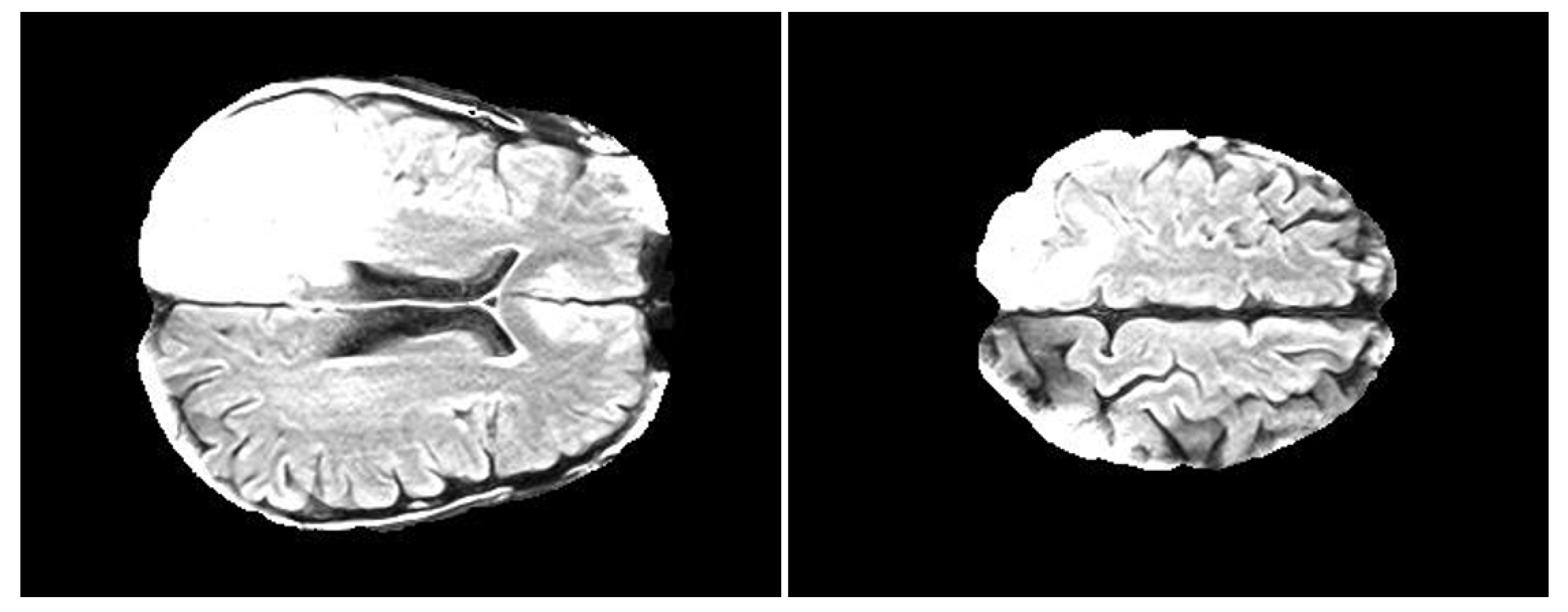
In particular, we are interested to detect and to study topological loops (1D, 2D, etc…) that would surround brain regions of interest. We have introduced a novel entropy, the so-called generator entropy, that is a function of the number of 0-simplices (vertices) in the loops. The comparison of a healthy brain with a pathological one by means of a FLAIR highlights that the latter is characterized by the presence of a mass with a different grey gradient which would correspond to a topological loop. If the mass structure is heterogeneous or if the brain is affected by multiple tumors the number of loops will be higher.

1.2. Paper Outline

The potential of radiomics to improve clinical decision support systems is widely accepted both among clinicians and data scientists. The principal challenge is the optimal collection and integration of diverse multimodal data sources in a quantitative manner without any subjective biases and to support the modeling steps aiming at both objective and reproducible clinical predictions [36]. In general with radiomics one refers to imaging data acquired at a single time-point, mostly imaging tumors before the beginning of treatment. Recently, a new approach called delta-radiomics has been introduced. In this setting, radiomics is augmented with temporal information throughout the course of treatment [37]. Current efforts are focused on the development of a new framework in which radiomics and delta-radiomics are combined with other clinical information that was collected over time. The framework is known as “picture archiving and radiomics knowledge systems” (PARKS). The system will provide technical and methodological indications towards personalized diagnosis and treatments. In order to build a PARK system several open challenges must be solved. Some of the challenges are technological (e.g., definition of standard format for data sharing, how to extract data from the electronic footprint of a single patients, and so forth). Other challenges are methodological, for example, how to generalize the model, how to consume data that are acquired with different resolutions, what features are needed for extracting insights from data produced at different spatial and temporal scales [36]. In Reference [38], the authors have used TDA for the analysis of GBM. The authors have presented a novel topological statistics that is suitable for predicting the survival of GBM patients. Among the conclusions, the authors have raised the problem that it would be worth investigating how to combine topological statistics with deep learning. Also, the authors believe that the analysis of tumor shape may help in distinguishing true progression from pseudoprogression. By pseudoprogressing they mean that the tumor has been infiltrated by immune cells and other factors. In the present investigation, we intend to demonstrate by means of numerical experiments that topological features shall be taken into account in the PARKS system and for proposing initial answers to the open questions presented in Reference [38]. In particular, we have executed three different experiments for showing that the same topological features can be enrolled for analysis at different time points as indicated by delta-radiomics (e.g., immediately after a treatment and after a follow-up period) and at different spatial scales, namely at a cellular level and at organ level and by using different data sources point cloud data or gray scale images. In particular, we have performed the following numerical experiments:

• Analysis 1—Topological Data Analysis of a simplified 2D tumor Growth Mathematical Model: identification how tumor growth over time is affected by the initial amount of available chemical nutrient
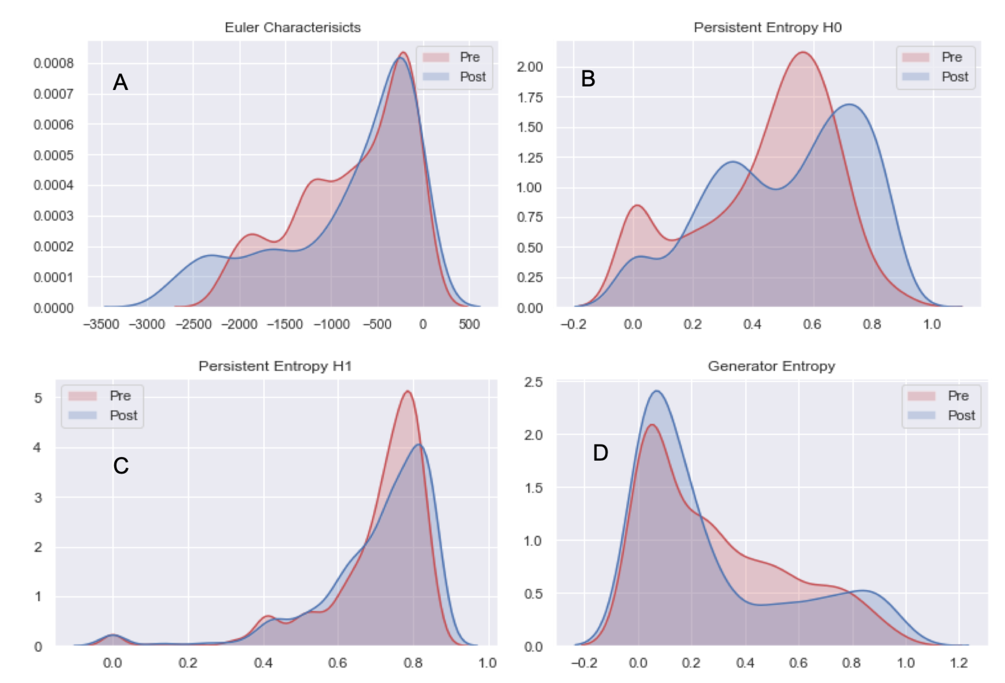
• Analysis 2—Topological analysis of Glioblastoma temporal progression on FLAIR: evaluation of GBM temporal evolution after treatment
• Analysis 3—Automatic GBM classification on FLAIR—the aims of this experiment is to evaluate the accuracy for classification GBM by characterization of 2D patches extracted from FLAIR by combining textural and topological data analysis with machine learning.

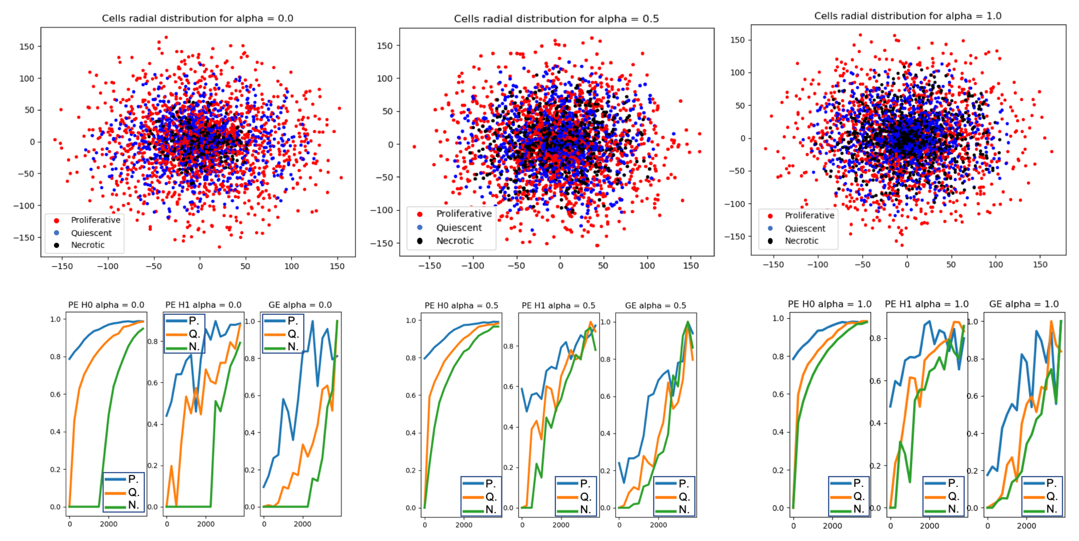
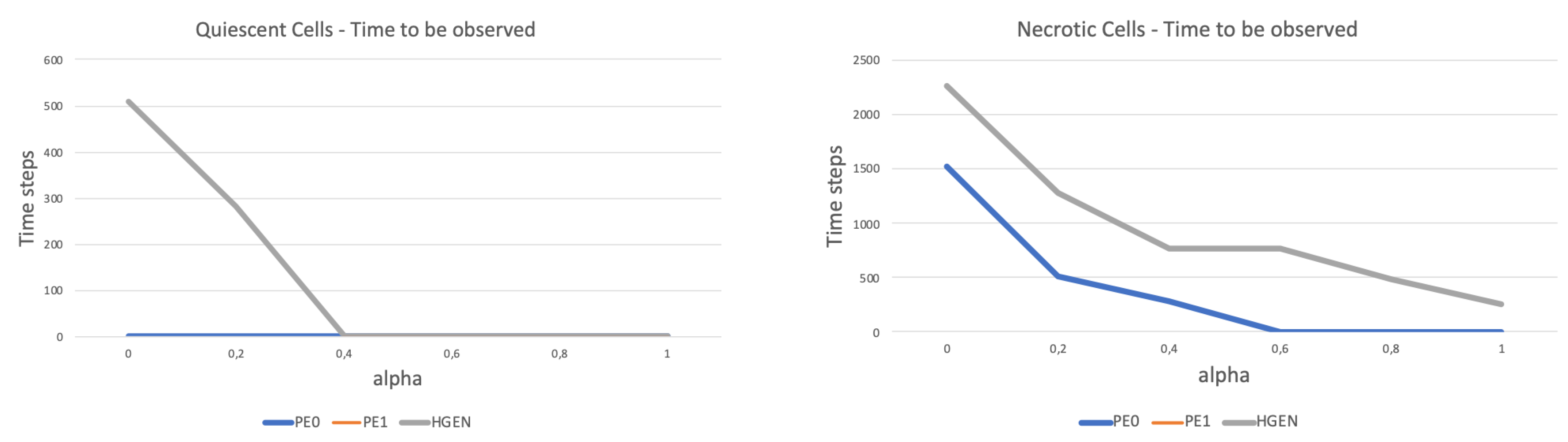
In the first experiment, we have integrated a discrete time mathematical model to study the evolution of three different types of tumor cells—proliferative, quiescent and necrosis. At each time step, we associated a point cloud data (PCD) to each cell set. The spatial evolution of the PCD is analysed by topological statistics, that is, persistent entropy. The plot of persistent entropy over time reveals interesting system evolution. The results encouraged us to analyse whether topological features can also detect GBM temporal evolution. To this extent, we have analysed a publicly available dataset that contains 2 sequences of FLAIR for 20 patients. The sequences were recorded within 90 days following chemo-radiation therapy (CRT) completion and at progression. The complete description of the dataset is in Section 2. For the sake of details, we have decided to use FLAIR since they reveal a wide range of lesions, including cortical, periventricular, and meningeal diseases that were difficult to see on conventional images. In the third experiment we have used the same dataset but for evaluating the possibility of discriminating healthy and pathological tissue on FLAIR, by the use of Statistical Texture Analysis and Topological Data Analysis. The discriminating power of statistical texture and of topological features was then exploited for the development of a supervised tumor detection methodology by means of automatic machine learning algorithms. We have adopted novel computational tools for debugging and understanding Machine Learning decisions.

For the sake of completeness, we notice the reader of the algorithms that were used in this paper are agnostic with respect to the use case and they can also be enrolled for the analysis of big-data problems in several application domains. In Reference [39], the authors have provided a survey of topological methods for the analysis of geometrical properties of big-data representing healthcare systems. We remark that topological data analysis can be executed both on point cloud data and on complex networks. Complex networks and possibly multi-layer networks are powerful tools for adding a structure to big-data [40]. Among others, TDA can be used for the analysis of complex networks and for revealing information at the meso-scale (i.e., between micro and macro) [41]. Machine learning represents the most used approach to model big data as described in References [42,43].

The paper is organized as follows—in Section 2, we introduce both the model for tumor-growth analysis used in the first experiment and the data-set for the second and third experiment. Also, we report on the preprocessing steps of the FLAIRs in the data-set. In Section 3, we recall the relevant background, namely the fundamental concepts of textural features and topological features. In Section 4, we provide the details for the execution of the three numerical experiments. In Section 5, we report on the the outcomes of the three experiments. Final thoughts about the results and next steps are discussed in the last Section 6.

2. Materials

2.1. Analysis 1: Topological Data Analysis of a Simplified 2D Tumour Growth Mathematical Model

In order to investigate the topological properties of tumor growth dynamics, we have used a well documented tumor growth model, the so-called Sherratt-Chaplain model [44]. The model is also valid for GBM like tumors [45]. The model describes the temporal evolution of cell densities of proliferating, quiescent and necrotic cells [46]. Cell movements (diffusion) are modeled by a competitive approach. The model has been updated and compared with in-vitro analysis for a fine-tuning of its parameters [47]. The motion equation for the proliferating p, quiescent q and necrotic cells n is:

$$\frac{dp}{dt}=\frac{\partial }{\partial x}\left(\frac{p}{p+q}\frac{\partial (p+q)}{\partial x}\right)+g\left(c\right)p(1-p-q-n)-f\left(c\right)$$

(1)

$$\frac{dq}{dt}=\frac{\partial }{\partial x}\left(\frac{q}{p+q}\frac{\partial (p+q)}{\partial x}\right)+f\left(c\right)p-h\left(c\right)q$$

(2)

$$\frac{\partial n}{\partial t}=h\left(c\right)q$$

(3)

where c is the concentration of some nutrients that can be represented by:

$$c=\frac{c_0\gamma }{\gamma +p}(1-\alpha (p+q+n)).$$

(4)

The functions $f,g$ and h are defined:

$$f\left(c\right)=\frac{1-tanh(4c-2)}{2}$$

(5)

$$g\left(c\right)=\beta e^{\beta c}$$

(6)

$$h\left(c\right)=\frac{f\left(c\right)}{2}.$$

(7)

The model can be solved with numerical methods by translating them into finite differences [47]. Under the assumption of radial symmetry the displacement of the cells can be seen as 2-dimensional. We remark that we do not intend to deep dive into the mathematical modelling of GBM growth, but we want to investigate topological properties of GBM like tumors.

2.2. Analysis 2 & 3: Dataset

In order to make our results comparable, analyses 2 and 3 were executed by using a public freely available dataset accessible via The Cancer Imaging Archive (TCIA) [48]. In detail, the dataset includes DICOM files of 20 subjects from different sites with primary newly diagnosed glioblastoma who were treated with surgery and standard concomitant chemo-radiation therapy (CRT) followed by adjuvant chemotherapy. The sequences are T1-weighted (pre and post-contrast agent), FLAIR, T2-weighted, ADC, normalized cerebral blood flow, normalized relative cerebral blood volume, standardized relative cerebral blood volume, and tumor masks (i.e., ROIs) [49,50]. Figure 1 shows two of the 2D slices contained in the dataset and extracted from FLAIR. Each patient is described by two MRI exams—within 90 days following CRT completion and at progression. At the best of our knowledge, in this paper the dataset is used for the first time for ML experiments [51]. The following preprocessing steps were performed before running the analysis:

2.3. FLAIR Preprocessing

The following preprocessing steps attempt to enhance and correct FLAIR for posterior analysis. We propose the following scheme for the dataset under analysis:

• DICOMs were transformed into NII files for enabling preprocessing steps (https://pypi.org/project/dicom2nifti/).
• FLAIRs were optimized by removing fat tissues and by performing skull stripping. The preprocessing steps, namely the removal of fat tissues and skull stripping, were performed by using the deep-learning algorithm described in Reference [52] (https://github.com/JanaLipkova/s3).

3. Background

3.1. Topological Data Analysis: Persistent Homology

Homology is an algebraic machinery used for describing a topological space $\mathfrak{C}$. Informally, for a fixed natural number k, the $k-$Betti number${\beta }_k$ counts the number of $k-$dimensional holes characterizing $\mathfrak{C}$: ${\beta }_0$ is the number of connected components, ${\beta }_1$ counts the number of holes in 2D or tunnels in 3D (here nD refers to the $n-$dimensional space ${\mathbb{R}}^n$), ${\beta }_2$ can be thought of as the number of voids in geometric solids, and so on.

Persistent homology is a method for computing the $k-$dimensional holes at different spatial resolutions. Persistent holes are more likely to represent true features of the underlying space, rather than artifacts of sampling (noise), or due to particular choices of parameters. For a more formal description we refer the reader to Reference [53]. In order to compute persistent homology, we need a distance function on the underlying space. This can be obtained constructing a filtration on a simplicial complex, which is a nested sequence of increasing subcomplexes. More formally, a filtered simplicial complex K is a collection of subcomplexes $\left\{K\right(t):t\in \mathbb{R}\}$ of K such that $K\left(t\right)\subset K\left(s\right)$ for $t<s$ and there exists $t_{max}\in \mathbb{R}$ such that $K_{t_{max}}=K$. The filtration time (or filter value) of a simplex $\sigma \in K$ is the smallest t such that $\sigma \in K\left(t\right)$. A $k-$dimensional Betti interval, with endpoints $[t_{start},t_{end}),$ corresponds to a $k-$dimensional hole that appears at filtration time $t_{start}$ and remains until time $t_{end}$. We refer to the holes that are still present at $t=t_{max}$ as persistent topological features, otherwise they are considered topological noise [54]. The set of intervals representing birth and death times of homology classes is called the persistence barcode associated to the corresponding filtration. Instead of bars, we sometimes draw points in the plane such that a point $(x,y)\in {\mathbb{R}}^2$ (with $x<y$) corresponds to a bar $[x,y)$ in the barcode. This set of points is called a persistence diagram. There are several algorithms for computing persistent homology and their analysis and for a complete overview of the available tools we refer to Reference [55].

3.2. Topological Features for Radiomics

In order to use persistent barcodes in any computer applications (e.g., machine learning), a set of numerical descriptors need to be derived, which encapsulate the information contained in the barcode. In the following we recall how to compute the statistics we use in this research. Two or more topological objects, for example, simplicial complexes, are homologically equivalent if they have the same sequence of Betti numbers. In other words by using persistent homology, they are characterized by the same number of persistent homological holes at each dimension. To facilitate the comparison of two or more simplicial complexes, one can calculate and compare the Euler Characteristics for each simplicial complex:

Definition 1 (Euler Characteristic). 

$$\chi =\sum _{i=0}^{i=n}{(-1)}^i{\beta }_i,$$

where ${\beta }_i$ is the Betti numbers at the i-th homological group (e.g., ${\beta }_0$ is the Betti number at $H0$ for counting the number of connected components, ${\beta }_1$ for counting the number of 2D holes, ${\beta }_2$ for counting the number of 3D empty volumes etc…).

Since Euler Characteristics are computed on the persistent homological holes and it discards completely the noisy topological features (i.e., not persistent) we suggest that to complement it, the so-called Persistent Entropy should also be computed. Persistent Entropy is a Shannon like entropy computed over the persistent barcodes and it is calculated by using both noisy and persistent topological features. It was defined initially in Reference [56] and further studies of its mathematical properties were published in References [57,58]. We recall its definition.

Definition 2 (Persistent Entropy). 

Given a persistence barcode $B=\{a_i=[x_i,y_i):i\in I\}$, the Persistent Entropy (PE) H of the filtered simplicial complex is defined as follows:

$$H=-\sum _{i\in I}{p}_{i}lo{g}_{10}\left(p_i\right)$$

where $p_i=\frac{{\ell }_i}{L}$, ${\ell }_i=y_i-x_i$, and $L={\sum }_{i\in I}{\ell }_i$.

In the case of an interval with no death time, $[x_i,+\infty )$, we truncate infinite intervals and replace $[x_i,+\infty )$ by $[x_i,m)$ in the persistence barcode, where $m=t_{\max }+1$.

Note that the maximum PE corresponds to the situation in which all the intervals in the barcode are of equal length. In that case, $H=logn$ if n is the number of elements of I. Conversely, the value of the PE decreases as more intervals of different length are present. A topological n-dimensional hole is generated by the so-called homological generator [59,60]. For example, a 1D hole is generated by a set of 0-simplices (vertices) linked by 1-simplices (edges). Given our interest to nD topological holes, we propose a new seminal statistics that is computed on the number of 0D simplices (vertices) in each topological feature.

Definition 3 (Generator Entropy). 

Given a filtered simplicial complex $\left\{K\right(t):t\in F\}$, and the collection of corresponding persistence barcode $B=\{a_i=[x_i,y_i):i\in I\}$ for the Homological Groups $H_j$ with $j\ge 1$.

$$GH=-{\Sigma }_{i=1}^{i=N}\left(p_{i}lo{g}_{10}\left(p_i\right)\right),$$

where N is the total number of homological lines in the barcode, $n_i$ is the number of 0-simplices in the i-th line and $L={\Sigma }_{i=1}^{i=N}{n}_i$ and $p_i=\frac{n_i}{L}$. For the sake of preciseness, in a topological loop there exist a 0-simplices that appears twice. In this setting we count each 0-simplices only once.

We envision that generator entropy as defined in Equation (3) could be used as a measure of the number of different objects of interests (e.g., tumors) surrounded by topological loops of in general different length.

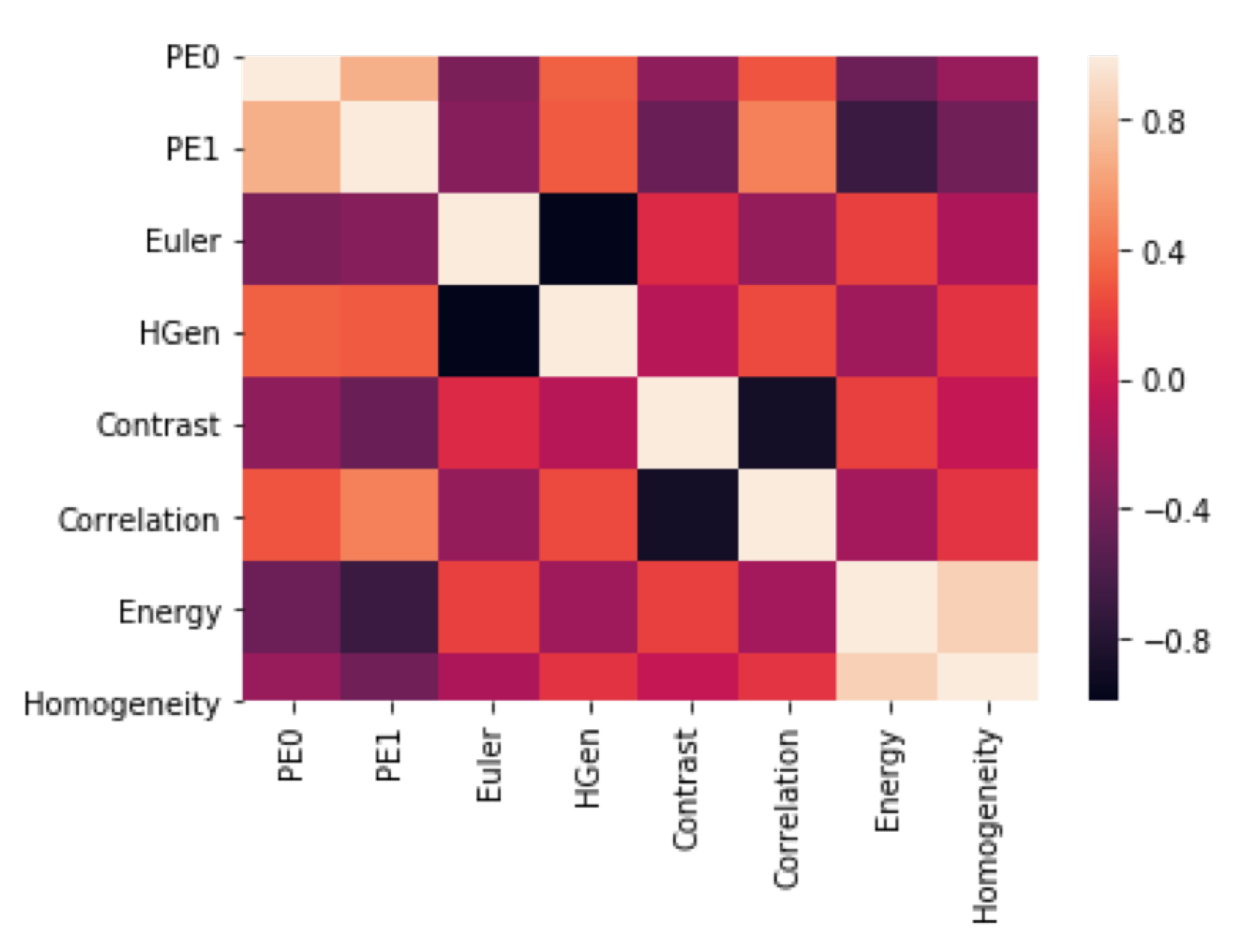
3.3. Textural Features: Grey-Level Co-Occurrence Matrix

In this study, we used one selected feature set (grey-Level Co-occurrence matrix (GLCM)) for the texture analysis in accordance with some previous reports of radiomics for GBM detection [61]. GLCM is a statistical method for examining image texture by taking into account the spatial relationship of pixels. The GLCM counts how often pairs of pixels with specific values and in a specified spatial relationship occur in an image. From GLCM we have extracted the following textural information [62]:

• Contrast—it measures the local variability in the grey level.
• Correlation—it measures the joint probability that a given pair of pixels is found.
• Homogeneity—it measures the distance between the GCLM diagonal and element distribution.
• Energy

In this paper, we have used the open-source software Ripser [63] (https://ripser.scikit-tda.org/) for TDA. Ripser allows us to compute the persistent homology of both point cloud data and 2D images. For the computation of persistent homology we have used a slightly modified version of the lower star filtration (https://ripser.scikit-tda.org/notebooks/LowerStarImageFiltrations.html). In our version, the algorithm computes the homology up to the first homological group and it returns for each topological loop a set of representative generators. While for GLCM computation we have used Scikit-Image [64].

3.4. Evaluation Metrics

We have evaluated the performances of the supervised machine learning and deep learning algorithms for patches classifications by different metrics:

• $Accuracy=\frac{TP+TN}{TP+TN+FP+FN}$
• $Precision=\frac{TP}{TP+FP}$
• $Recall=\frac{TP}{TP+FN}$
• $F1=\frac{2TP}{2TP+FP+FN}$
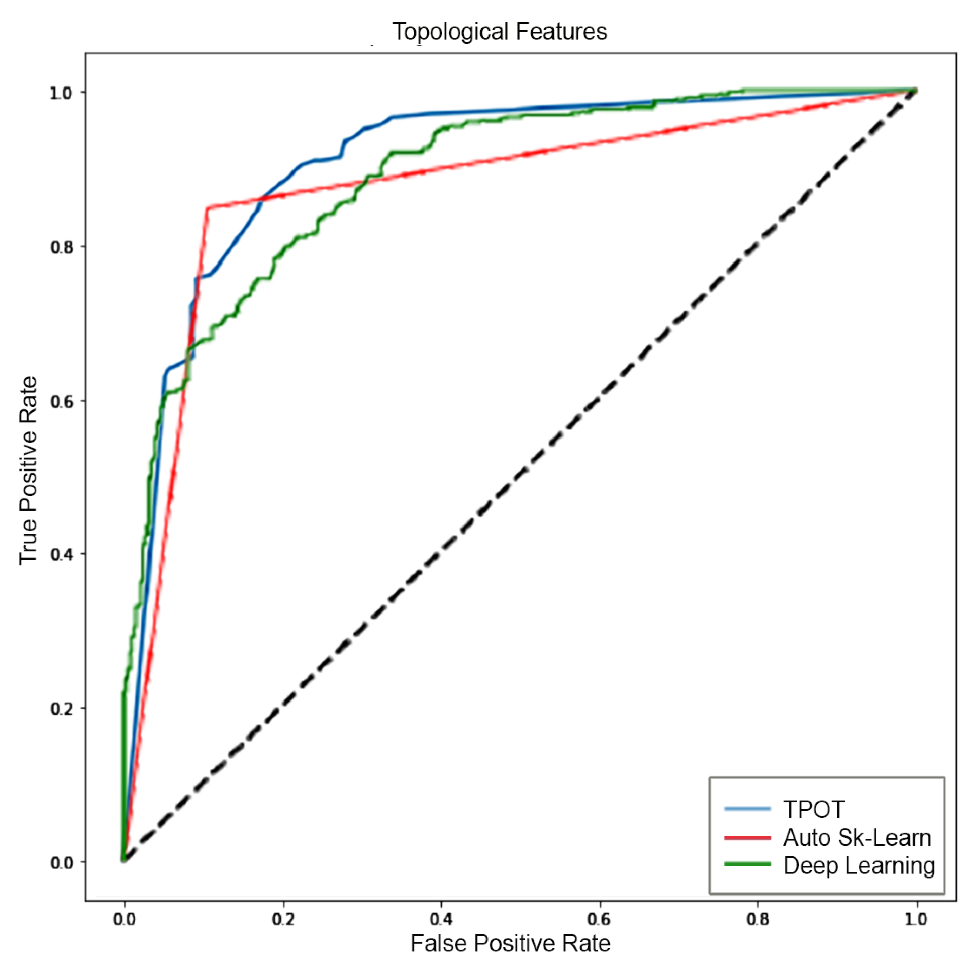
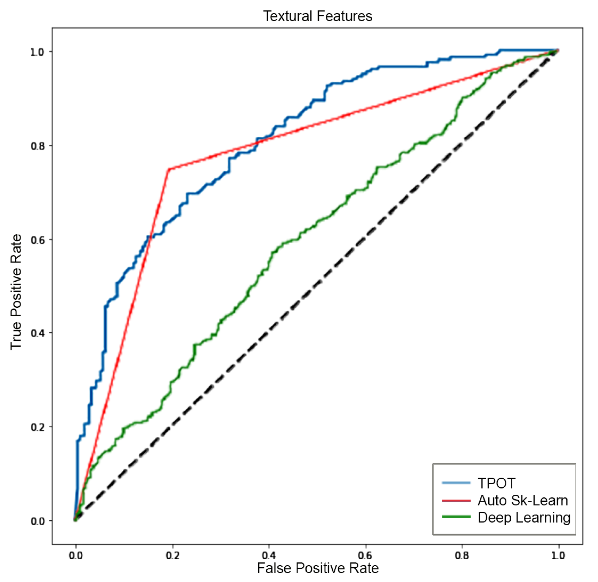
• AUC is the area under the receiver operating characteristics curve (ROC). The ROC is obtained by plotting of the true positive rate ($TPR=\frac{TP}{TP+FN}$) against the false positive rate ($FPR=\frac{FP}{FP+TN}$) at various threshold settings [65].

where, $TP$ refers to the true positives in the classification, $TN$ to the true negatives, $FP$ to the false positives and $FN$ to the false negatives. A model with extremely poor performances has AUC near to 0, while a model with excellent performances has AUC near to 1. In the middle, when AUC is 0.5, it means the model has no class separation capacity whatsoever.

3.5. Computational Complexity

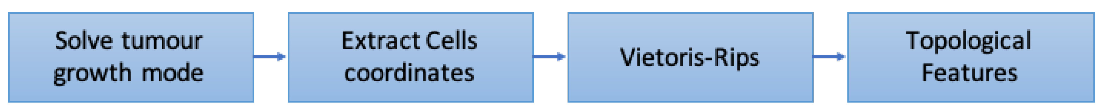
Vietoris-rips complexes are used in all three experiments. Building a Vietoris-Rips simplicial complex can be at worst exponential in the number of vertices, as the complete simplicial complex on n vertices has $O\left(2^{n-1}\right)$ simplices. This indicates that one must limit the size of a Vietoris-Rips simplicial complex construction. There have been a few recent efforts aiming to optimize the complexity of persistent homology computation and/or to provide implementations that are suitable for GPU [66,67]. An interesting solution for taming computational complexity is proposed in Reference [68]. The authors designed an algorithm with a computational complexity of $O\left(n^2\right)$. It will be worth investigating this solution for the deployment of a run-time implementation of the framework proposed in this paper. The computational complexity of persistent entropy and of generator entropy is proportional to $O(2\ast n)$, where n is the number of lines in the persistent barcodes. For the sake of completeness, the basic version of the algorithms for their computation would be based on two main loops over the lines in the barcode: 1) the first iteration is needed for computing the total length of the lines (or the total number of unique generators); 2) the second iteration is needed for computing the ratio of the single line with respect to the total length and for accumulating the product of line length times the ratio. The computational complexity of GLCM features, we remark that it depends on the number of gray levels G and is proportional to $O\left(G^2\right)$ [69]. The computational complexity of a Machine Learning algorithm depends on the algorithm itself, the number of parameters and the unique samples in the input space. Also, the computational complexity of the training procedure is in general different with respect to the testing [70].

4. Methods

4.1. Analysis 1: Topological Data Analysis of a Simplified 2D Tumor Growth Mathematical Model

We have integrated the model introduced in Section 2.1 by using the code provided in Reference [47] but rewritten in Python. The dimensionless parameters $\alpha$, $\gamma$ and $\beta$ are extracted from in-vitro experiments. We remark that $\alpha$ and $\gamma$ represent concurring with the definition of the initial concentration of chemical nutrient. We have analysed how the system is affected by different values of $\alpha$ by keeping $\gamma =10.0$ and $\beta =0.5$. For each value of $\alpha$, and throughout the integration, the 2D coordinates of each cell were extracted. The coordinates were used as input for TDA. Figure 2 is representative of the main steps in the experiment, which are:

• Solve tumor growth model over different $\alpha$.
• Extract cells coordinates.
• Embed the coordinates in a space equipped with the Euclidean metrics and compute Vietoris-Rips simplicial complexes.
• Compute topological features: persistent entropy at H0 and H1, and Generator Entropy.
• Plot the topological features vs $\alpha$.

Figure 3 depicts both the spatial distribution of the cells and the corresponding topological features computed throughout the system’s integration.

4.2. Analysis 2: Topological Data Analysis of Tumor Progression

The dataset contains for each patient two MRI exams—the exams were recorded within 90 days following CRT completion and at progression, for now on “pre” and “post”. For each patient the topological features (i.e., Euler characteristics, persistent entropy at H0 and H1 and generator entropy) were computed on the 2D slices of FLAIR. Welch’s t-test is used for comparing the mean of the topological descriptor computed over the “pre” and “post” set of images. A pictorial representation of the main steps in this experiment are represented in Figure 4. We recall the steps that were executed are:

• From both preprocessed “pre” and “post” FLAIRs (i.e., after skull stripping) extract all the slices containing the tumor according to the corresponding ROIs.
• For each slice compute the 2D lower star filtration.
• Compute Topological features: Euler Characteristics, Persistent Entropy at H0 and H1 and Generator Entropy at H1.
• Compare the distributions by using statistical tests, that is, t-test and p-value.

Figure 5 depicts two FLAIR slices extracted for the same patients within 90 days following chemo-radiation therapy (CRT) completion and at progression, “pre” and “post” as labeled in the text.

4.3. Analysis 3: GBM Classification

In this work, we have implemented and tested the following GBM classification methodology using texture and topological data analysis. The inputs for the methodology are the FLAIR and the corresponding ROI files. Figure 6 depicts the process that was executed for each 2D slice extracted from the preprocessed FLAIRs:

• 2D GLCM features and topological features were calculated with a sliding patch approach in the segmented ROI. The size of the patch is $30\times 30$.
• In order to identify discriminating features, the same feature calculations were also performed in the contralateral (healthy) ROIs.
• Each sliding patch was labeled as healthy or ill according to the class of its ROI. Each patch was also stored for future analysis.
• Features selection.
• The dataset is randomly divided into training and testing subsets that contain the 70% and 30% of samples, respectively.
• The training set is used for training a machine learning classifier. For the sake of completeness, during training we adopted a k-fold cross validation standard procedure [71] (https://machinelearningmastery.com/difference-test-validation-datasets/) with $k=5$.
• Splitting, training and testing procedures were executed multiple times by using different set of features—only topological features or only GLCM features or topological plus GLCM features.
• Classifier behavior is debugged by tools from information theory. This allows to understand feature relevance and to understand what are the numerical input characteristics related to the classification verdict. Specifically, we have used Skater and Lime algorithms [72] (https://www.oreilly.com/ideas/interpreting-predictive-models-with-skater-unboxing-model-opacity).

Figure 7 provides a graphical detail of the steps $\#1$ and $\#2$ of the process. In particular, it shows the extraction of the ROI and of its controlateral. The cells shaping the grids are the patches. From each patch the topological and the textural features are extracted and stored into a table. Each patch is labeled accordingly to its source—ill or healthy ROI.

4.3.1. Feature Selection

Feature extraction comprises the process of extracting new features from the FLAIR. For each patch, eight features (four topological plus four texture features) were computed. Features were standardized by removing the mean and scaling to unit variance (https://scikit-learn.org/stable/modules/generated/sklearn.preprocessing.StandardScaler.html). Spearman’s rank-order correlation combined with backward elimination was used to calculate the correlations between features and outcome variables. Features with the highest correlation and p-value ≤ 0.05 become more expressive of GBM characteristics. Figure 8 depicts the correlation among the features. Topological features are quite correlated among them. We observe that “generator entropy” (HGen) shows a positive correlation with “homogeneity”. This is in line with the idea that HGen is affected by how much the image is homogeneous both in terms of structure and in terms of grey distribution. Eventually, the correlation analysis has selected seven out of eight features. For the sake of completeness, all the topological features were selected while the textural features correlation were discarded. Figure 9 depicts the density distribution of the features that were selected. The topological features “persistent entropy” for H0 and for H1 groups and the textural feature “homogeneity” show a quite good separation between the ill (red) and healthy (green) group. The other features show different peaks but their distributions are overlapped.

4.3.2. Machine Learning Algorithm Selection

The selection of the ML algorithm was performed by using an Automatic Machine Learning tool, that is, Auto-Sklearn [73] and TPOT [74]. Auto-sklearn uses Bayesian optimization approaches for the automatic selection of the machine learning classifier based on an ensemble of scikit-learn algorithms. Auto-sklearn compares and ranks different solutions and returns the solution that maximizes the accuracy. TPOT is a framework that uses a genetic algorithm for comparing different machine learning solutions and it automatically finds the best pipeline that maximizes the accuracy. Both Auto-Sklearn and TPOT produce a pipeline containing both preprocessing steps—if needed—and the selected Machine Learning architecture.

4.3.3. Deep Learning Approach on Numerical Features

For the sake of completeness, we have also trained deep learning classifiers on the selected features. In particular, we have trained multiple models with an architecture based on sequential dense layers with a rectified linear unit (relu) activation function, followed by a dropout layer for preventing over-fitting and eventually by another dense layer as an output layer. The difference among the models is the number of dense layers before the dropout and the number of neurons per layer.

4.3.4. Gbm Classification—Deep Learning Approach on Patches

Deep-learning based solutions are opening new doors in the field of GBM detection and segmentation. We have compared the performance of the machine learning solution with two different Deep Neural networks on the patches extracted in the methodology defined in Section 4. Figure 10 contains 8 out of 1612 patches used for training and testing the algorithms. The first network contains 4 alternating convolutional and max-pooling layers, followed by a dropout after every other convolutional-pooling pair. After the last pooling layer, the network contains a fully-connected layer with 256 neurons, another dropout layer, then finally a softmax classification layer for two classes (i.e., pathological and healthy). The loss function is the categorical cross-entropy loss, and the learning algorithm is the AdaDelta. The network contains about 1 million parameters. In the second setup, we have executed the transfer learning of a pre-trained VGG16 model. Transfer learning means the adaption of a pre-trained and optimized deep learning architecture for dealing with our dataset. The model consists of several convolutional layers, followed by some fully-connected/dense layers and then a softmax output layer for the classification. The dense layers are responsible for combining features from the convolutional layers. In this experiment, another dense-layer and a dropout-layer were added to avoid over-fitting. VGG16 contains 13 convolutional layers and two fully connected layers at the end, and it counts more than 138 million parameters. VGG16 was made to solve ImageNet, and achieves an $8.8\%$ top-5 error rate, which means that $91.2\%$ of test samples were classified correctly within the top 5 predictions for each image. The network was adapted to the two classes classification by removing the original final classification layer, which corresponds to ImageNet, which was replaced by a new softmax layer which contains 2 neurons. Keras implementation of VGG16 facilitates handling such a huge network and it optimizes memory issues [75]. Both networks were trained for 100 epochs with a batch size of 128. For both networks, Keras API for TensorFlow and Google Colab environment (https://colab.research.google.com/github/kylemath/ml4a-guides/blob/master/notebooks/transfer-learning.ipynb) were used for the training.

5. Results

5.1. Analysis 1: Topological Data Analysis of a Simplified 2D Tumor Growth Mathematical Model

Figure 3 (top) depicts cells’ spatial displacement for $\alpha =[0.0,0.5,1.0]$ and the corresponding topological statistics (bottom) computed throughout system integration. At first look, with low $\alpha$, the quiescent and necrotic cells (in blue and black respectively) are quite confined in the central region, while for high $\alpha$ they are more scattered. We have further investigated this aspect by plotting for different $\alpha$ the amount of time steps that were needed to find topological features greater than zero. Since proliferative cells are always present and thus the corresponding topological features are immediately greater than zero, we have focused our analysis only on quiescent and necrotic cells. The outcome of the analysis is represented in Figure 11. At a high concentration of nutrients $\alpha \ge 0.4$ the phenomenon is more virulent and therefore it takes less time for proliferating both quiescent and necrotic cells.

5.2. Analysis 2: Topological Data Analysis of tumor Progression

Topological features detect the change of brain shape between the “pre” and “post” CRT treatment. Figure 12 describes the density estimation for the topological features (Euler Characteristics, Persistent Entropy for Ho and H1 and Generator Entropy). It is well evident that the two distributions of persistent entropy for the connected components (H0) are quite different—the distribution for the “pre” set (red) is bimodal with a local maximum at 0.0 and a global maximum ≈ at 0.6. The distribution for the “post” set (blue) contains two local maxima and a global maximum ≈ at 0.7. Welch’s t-test was computed for testing the null hypothesis that the means of the distribution are equal. The outcome of the analysis is capture in

Table 1. Statistical analysis of topological features for tumor progression analysis.

Topological Statistics
	Pre	Post	t-Test	p-Value
Euler Characteristics	−773.94 +/− 62.98	−830.31 +/− 74.55	1.84	0.06
Persistent Entropy H0	0.44 +/− 0.23	0.51 +/− 0.24	−6.79	0.01
Persistent Entropy H1	0.70 +/− 0.15	0.70 +/− 0.16	−0.29	0.77
Generator Entropy H1	0.30 +/− 0.26	0.28 +/− 0.27	1.68	0.09

. Only the distributions for the persistent entropy at H0 are statistically different. This result would suggest using persistent entropy as a new measure for monitoring the follow-up of chemo-radiation therapy (CRT) treatment for GBM.

5.3. Analysis 3: GBM Classification on FLAIR

Table 2. Machine Learning Accuracy—Topological Features.

Topological Features
	TPOT		Auto Sci-Kit Learn		Deep Learning
Metric	Train	Test	Train	Test	Train	Test
Accuracy	0.89	0.84	0.97	0.87	0.82	0.79
Precision	0.88	0.83	0.97	0.88	0.90	0.91
Recall	0.88	0.84	0.96	0.84	0.72	0.67
Misclassification rate	0.10	0.16	0.03	0.13	0.17	0.20
F1	0.89	0.83	0.97	0.88	0.80	0.77
AUC	0.89	0.89	0.97	0.87	0.82	0.79

,

Table 3. Machine Learning Accuracy—Textural Features.

Topological Features
	TPOT		Auto Sci-Kit Learn		Deep Learning
Metric	Train	Test	Train	Test	Train	Test
Accuracy	1.00	0.71	0.93	0.77	0.60	0.58
Precision	1.00	0.70	0.94	0.78	0.61	0.60
Recall	1.00	0.71	0.92	0.74	0.51	0.51
Misclassification rate	0.00	0.28	0.07	0.23	0.40	0.42
F1	1.00	0.71	0.93	0.76	0.56	0.55
AUC	1.00	0.81	0.93	0.77	0.60	0.57

and

Table 4. Machine Learning Accuracy—Topological and Textural Features.

Topological Features
	TPOT		Auto Sci-Kit Learn		Deep Learning
Metric	Train	Test	Train	Test	Train	Test
Accuracy	0.96	0.89	0.98	0.92	0.90	0.89
Precision	0.96	0.89	0.99	0.95	0.87	0.85
Recall	0.95	0.89	0.97	0.87	0.93	0.84
Misclassification rate	0.04	0.10	0.02	0.08	0.09	0.15
F1	0.96	0.89	0.98	0.91	0.90	0.84
AUC	0.99	0.96	0.98	0.91	0.90	0.84

show the results obtained in the training and test sets respectively, grouped by the algorithms tested in this study. The corresponding ROC curves are depicted in Figure 13, Figure 14 and Figure 15. In detail, Table 2 contain the figure of merit for the classifiers trained over the topological features. Auto SciKit Learn is performing extremely well on the training set but its performances are less good on the test set; this might be a consequence of overfitting. TPOT performances on the training set are worse than Auto SciKit Learn but the performances on the test set are quite similar, thus TPOT does not suffer from overfitting. This behavior is also observed in Table 3 and Table 4. This interpretation is confirmed by looking at the ROCs depicted in Figure 13, Figure 14 and Figure 15. We note that the closer the curve follows the left-hand border and then the top border of the ROC space, the more accurate the test. The ROCs for TPOT are closer to the point of coordinates $(0,1)$ which means they correspond to accurate tests. The worse performances are obtained by using only the textural features and the worst performances are obtained by the deep learning solution. The ROC of deep learning (Figure 14) falls down in situations in which the closer the curve comes to the 45-degree diagonal of the ROC space, the less accurate the test. The combination of topological and textural features reached the best performances with $AUC=0.96$ for the test set (Figure 15). In general, TPOT shows a better performance because it optimizes over more parameters and thus it increases the separation of the features with respect the two classes. Similar results were found in Reference [76].

Machine Learning Classification Interpretation

Skater and Lime algorithms were used for computing features relevance with respect to the TPOT machine learning algorithms trained on topological and textural features [72]. The output of Skater is depicted in Figure 16. For the TPOT classifier, the textural features homogeneity have the same relevance of the topological entropy persistent entropy at H0 - PE0 that is followed by generator entropy—HGEN. This confirms that the combination of topological and textural features were allowed to reach high accuracy. The less relevant features is contrast; however, since its importance is greater than 0 it cannot be discarded.

The output of Lime is represented in Figure 17. The Lime algorithm has allowed us to understand what the numerical characteristics are for a patch to be classified as healthy or ill. Negative (blue) indicates healthy tissue, while positive (orange) indicates ill tissue. The way to interpret the weights by applying them to the prediction probabilities is straightforward. The bars indicate the weight for each feature and the corresponding value for the slice under test. The subtraction of the weights from the prediction probabilities (1 in both cases as indicated in the left part of the picture) will alter the probability of a sample to be classified ill or healthy. This highlights that even if some features might appear globally less relevant, they are fundamental for avoiding “flipping coin” predictions.

5.4. GBM Classification with Deep Learning

Table 5. Deep Learning Accuracy using patches.

Deep Learning on Patches
	VGG16 Transfer Learning		Ad-Hoc
Metric	Train	Test	Train	Test
Accuracy	0.99	0.97	0.74	0.75
Precision	1.00	0.99	0.67	0.66
Recall	0.98	0.95	0.97	0.95
Misclassification rate	0.01	0.03	0.26	0.25
F1	0.99	0.97	0.79	0.78
AUC	0.99	0.97	0.74	0.77

shows the results obtained in the training and test sets respectively, grouped by the deep learning algorithms tested in this study. The corresponding ROC curves are depicted in Figure 18. The fine-tuning of VGG16 with the transfer-learning approach has allowed us to reach the best performances. By comparing the metrics (e.g., accuracy, precision-recall, misclassification rate and F1) it is evident that VGG16 outperforms TPOT. Only the AUC of TPOT ($96\%$) is quite close to the AUC reached by VGG16 ($97\%$). Finally, examples of patches classification achieved by applying the fine-tuned VGG16 on an entire 2D FLAIR is shown in Figure 19.

6. Discussion

Topological data analysis is a reliable approach to shedding light on GBM characteristics, as has been demonstrated by the three numerical experiments described in this paper. For the sake of precision, the main limitation of our work is due to that persistent homology can be computed only over one proximity parameter at a time and thus it does not allow us to study how the topology of the simplicial complexes changes along two or multiple directions. This limitation should be taken into account if one intends to use persistent homology for dealing with 3D tumor analysis. In general a tumor does not follow a $3D$ isotropic distribution but instead it shows a different growing rate along the axis. Fast and reliable assessment of GBM presence is critical for an accurate surgical and radiotherapy planning as well as to evaluate and quantify treatment-related effects and progression In the recent period, surgical approaches are strongly changed, with a progressive shift from classical neurosurgical techniques towards newer approaches with surgical navigation systems fluorescence-guided and MR-guided surgery [2,3,77]. Also, chemotherapy employed techniques with wafer drugs positioning in situ to minimize systemic collateral effects [78]. Consequently, radiological techniques able to localize and evidence every minimum GBM localization are essential to enforce new therapeutic possibilities that can improve the extent of tumor resection, prolong survival and increase the quality of life.

We note that the three single experiments should be seen as seminal efforts for making possible the paradigm of a personalized characterization and diagnosis of GBM. To the best of our knowledge, this paper presents for the first time the application of topological data analysis for the analysis of tumor growth model and for quantifying the temporal evolution of GBM from FLAIR and this makes a direct comparison with other works difficult. The same paradigm but with a different approach was presented in Reference [79]. In Reference [79], the authors proposed a very interesting framework obtained by combining a 3D continuous mechanical model, able to simulate the growth of a glioblastoma and the invasion of the surrounding tissue. The model produces high fidelity results since it it takes into account both the heterogeneity and the anisotropy of the brain tissues directly from DTI data. In our work, topological descriptors such as Euler Characteristics, Persistent Entropy and Generator Entropy were used to identify the physiological conditions that facilitate tumor growth. We notice that Generator entropy was introduced in this paper as a novel topological statistic that summarizes the number of homological generators of $nD$ homological loops. In particular, topological statistics were able to identify the change of proliferation rate of quiescent and necrotic cells as a consequence of nutrient concentration—the higher the concentration of chemical nutrients the more virulent the process. We would promote our approach as a data-driven solution rather than a model-driven solution, in real life applications, the simple model that we have used for generating cells distribution should be substitute with observations, that is, cells counting. In our opinion, the application of TDA to dynamical systems representing GBM tumor growth in the brain would let interesting results. Specifically, besides detecting the bio-chemical conditions, TDA should identify topological constraints (e.g., anatomical characteristics) that provide a personalized characterization of the tumor.

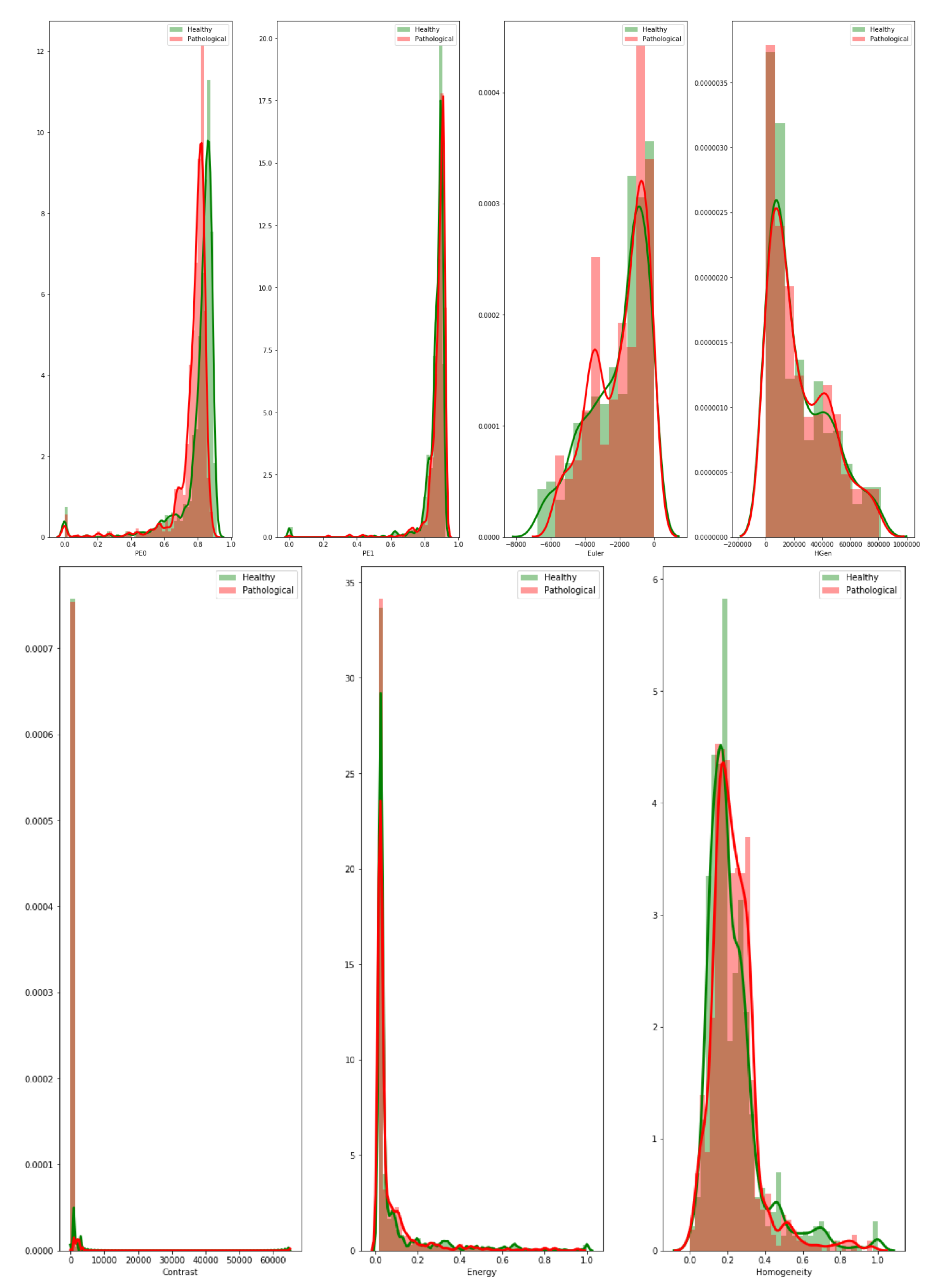
In the other two experiments, we demonstrated by using a publicly available dataset that topological features can be used as new radiomics features for GBM characterization. The analysis of FLAIR sequences recorded within 90 days following chemo-radiation therapy (CRT) completion and at progression by means of topological descriptors has confirmed by statistical test that persistent entropy computed at the homological group H0 of the connected component is a viable alternative for monitoring treatment effects. In Reference [80], the authors demonstrated that textural features combined with machine learning are a viable approach for the analysis of GBM follow-up progressive and responsive forms. We believe that TDA should be used for complementing this approach for the analysis of GBM during the follow-up period since TDA will reflect geometrical properties that otherwise would not be observed. 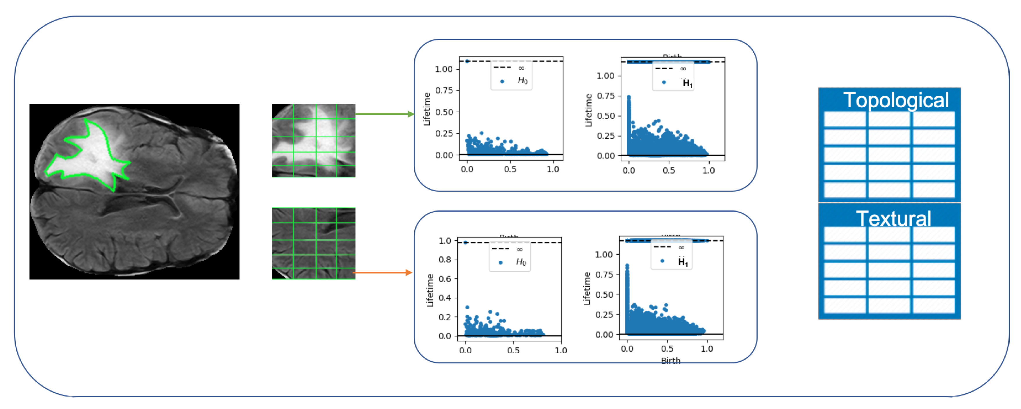In Reference [38], the authors defined a new topological statistics for predicting the survival of GBM patients while we focused on the classification of patches from FLAIR and/or to evaluate the evolution of GBM within a follow-up period. Among the open questions, they posed the challenge “how to combine topological features with machine learning?” We have shown a possible solution by extracting the sliding patches and by computing TDA on them that became a subset of the input features for the machine learning algorithm.

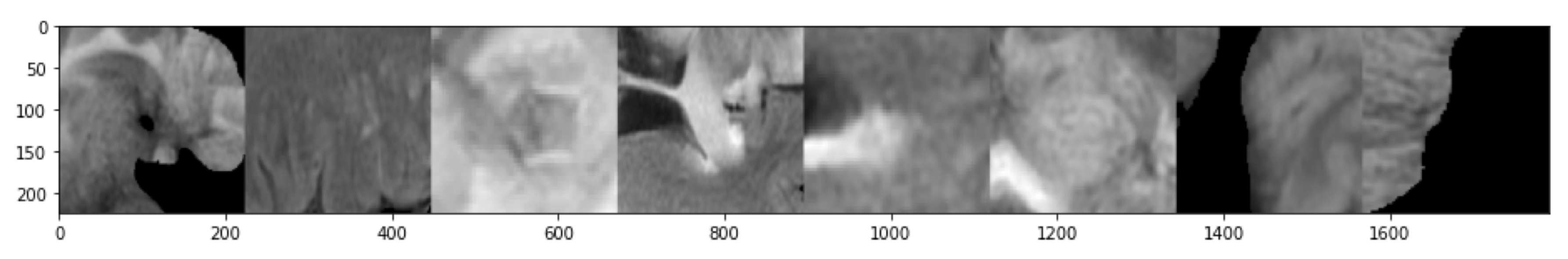
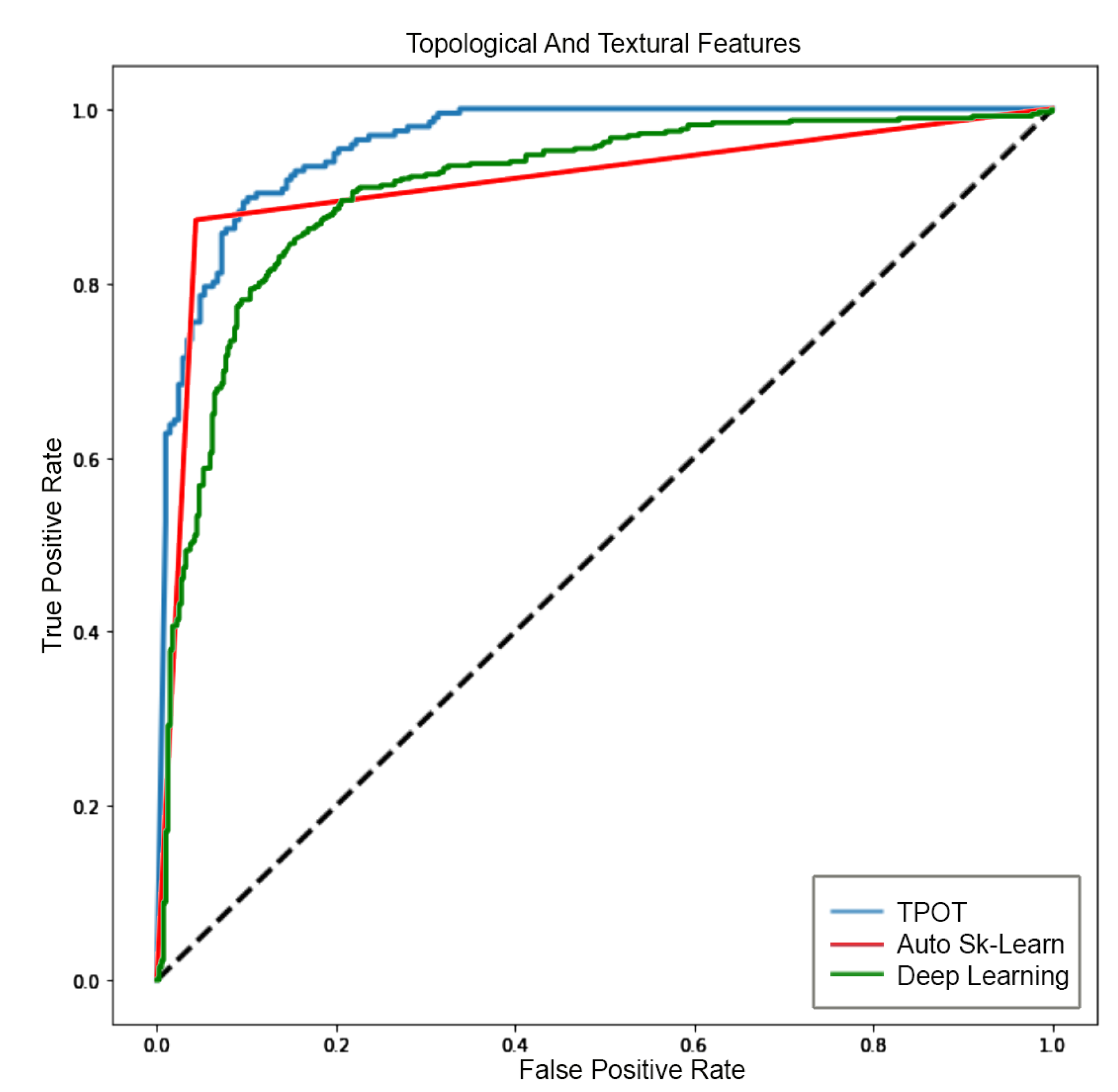
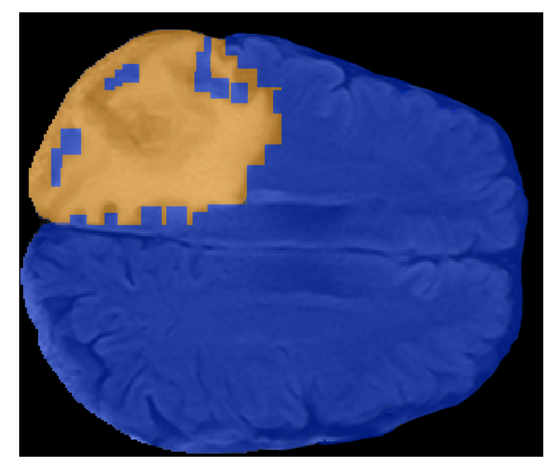
Based on these results, we proposed a new method for GBM analysis. The supervised method for automatic classification of 2D patches extracted from FLAIR sequences is a viable alternative for GBM identification. The proposed method comprises the following main stages—image preprocessing, sliding patches extraction, topological and textural features computation and selection, supervised classification via automatic machine learning, interpretation of classifier prediction. Preprocessing steps, that is, skull stripping, were obtained by employing the latest deep learning technology. Several supervised classification algorithms were evaluated to ensure the highest classification accuracy. To this extent, two different automatic machine learning selection frameworks were evaluated, which are TPOT and Auto-SkLearn. Python notebooks will be made available upon request to the authors. The algorithms were trained using topological features or textural features or the combination of the two sets. The selected machine learning approaches were used as a baseline in the comparison with deep learning based approaches. For the sake of completeness, deep learning approaches were trained on the same features set or directly on the patches (sub-images) extracted from the 2D FLAIR. The quality of classification was assessed by several metrics and ROC curves. 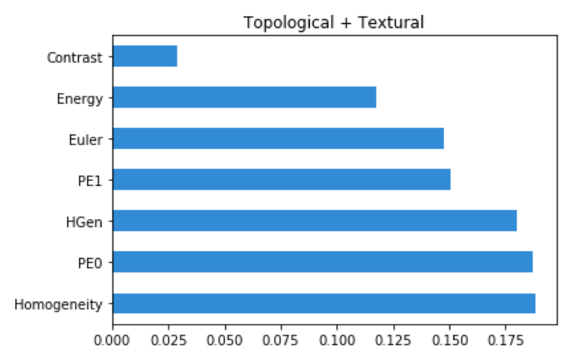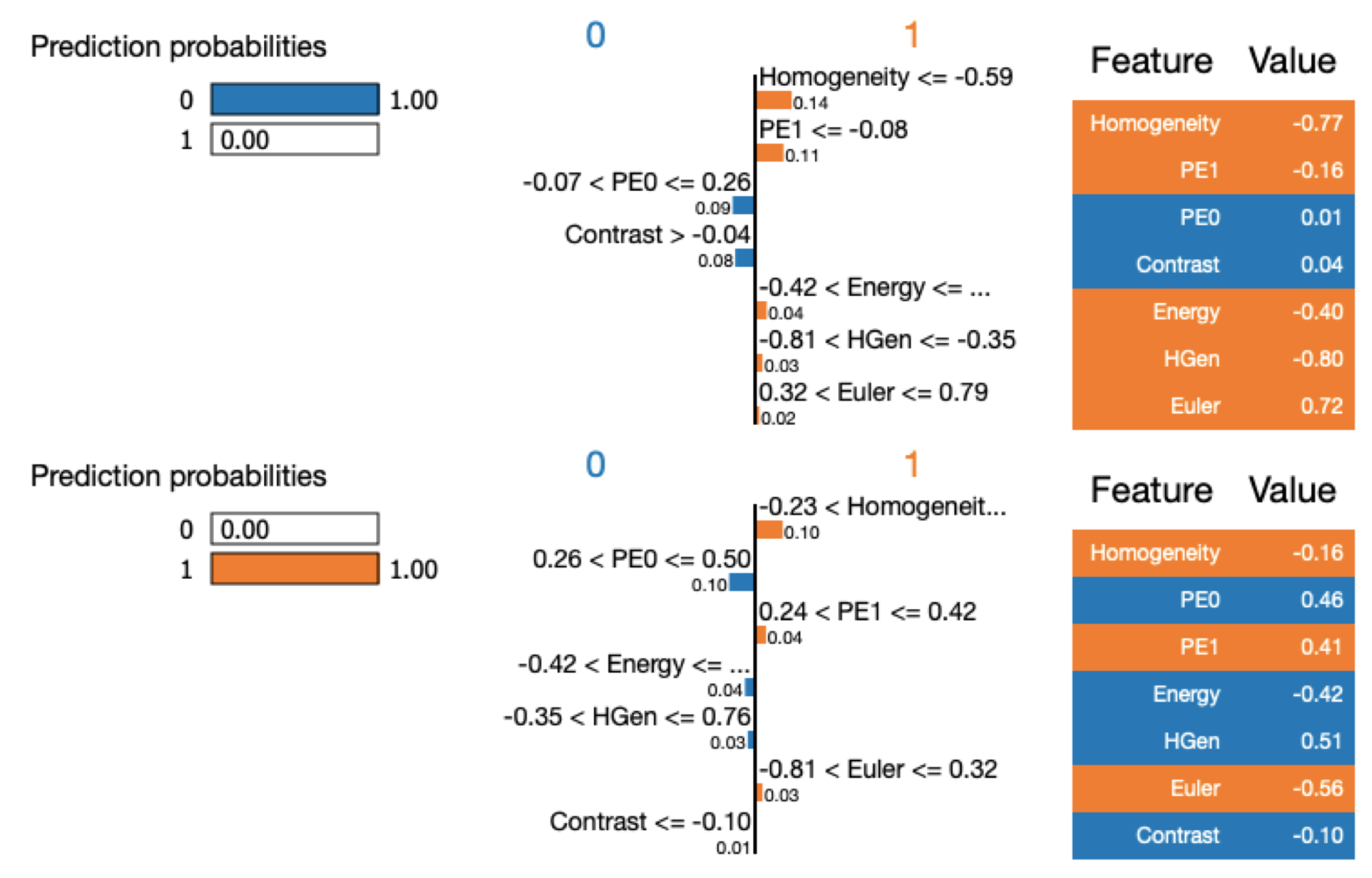The highest accuracy using the features was reached by TPOT trained on the two sets (e.g., topological and textural) with an accuracy of $89\%$ and $AUC=96\%$. 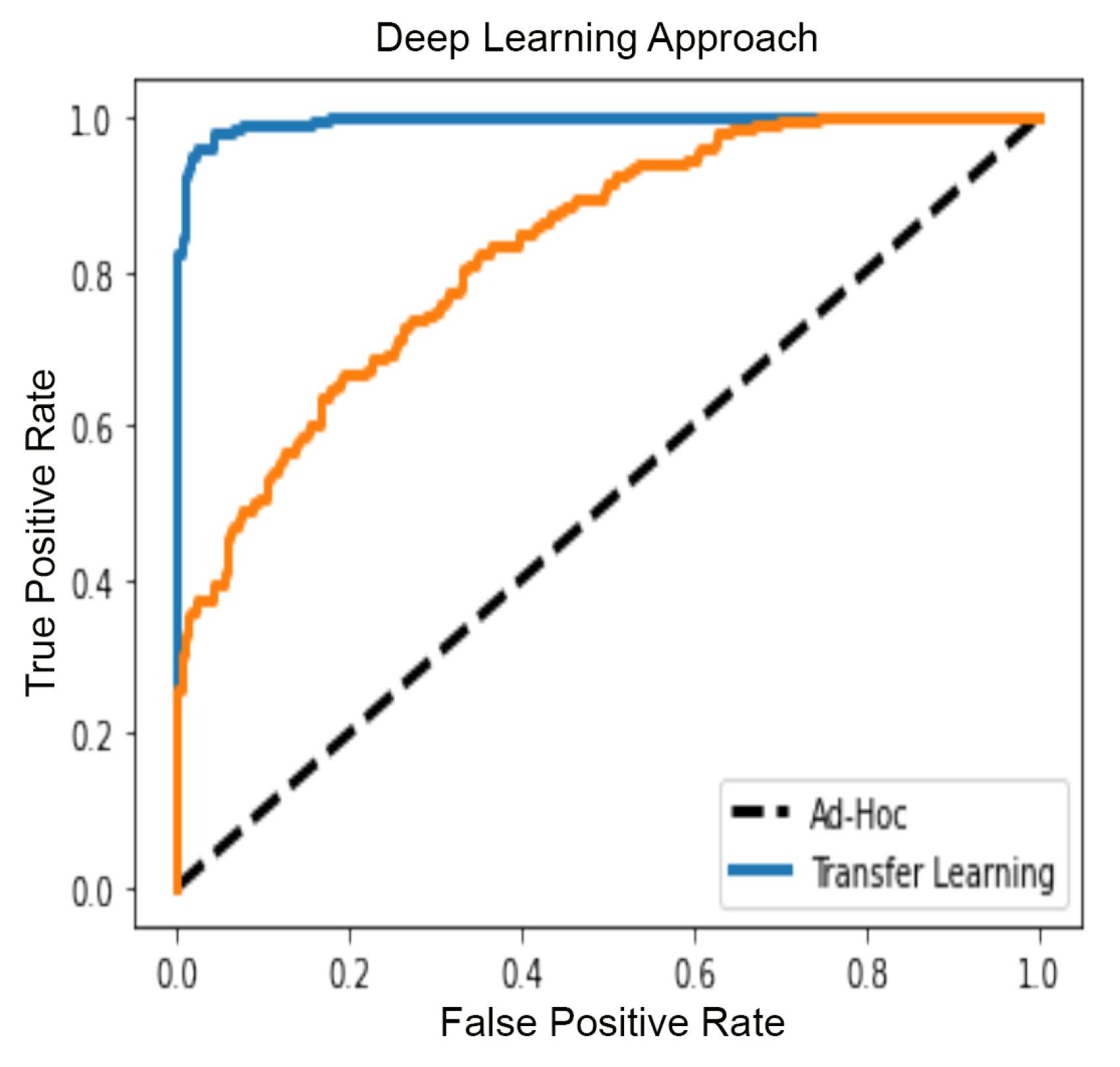Finally, the trained systems were investigated with tools from information theory. Skater and Lime algorithms allowed computing features relevance and for understanding what are the numerical characteristics of a patch to be classified ill or healthy. The interpretation has confirmed the importance of topological features. The transfer learning of a pre-trained VGG16 network that allowed for patches classification had allowed us to reach an accuracy of $97\%$ and $AUC=97\%$. However, we would like to remark that in general, Deep Learning based methods require ad-hoc hardware for their training, in fact we have used the Google Colab platform that allows access to both GPU and TPU units. The adoption of a deep learning solution would be straightforward, but we note that machine learning classification verdicts can be easily interpreted by enrolling tools like Skater and Lime, while the interpretation of the feature space extracted by a deep learning solution might be unfeasible, since the convolutional features might not correspond to any physical information. Even if we have reached good classification accuracy, our approach does not take into account anatomical context. We encourage the reader to consider deep Learning solutions for GBM classification and segmentations. These algorithms can be trained directly on the $3D$ volume. Among the solutions, it is worth considering the results presented in Reference [81] in which the authors have trained a U-net network on images from BRATS 2018 and they have demonstrated that the same network can be used for the identification of the whole tumor, the enhancing tumor and the tumor core with great accuracy—$0.908\%,0.784\%,0.844$ respectively, while the method proposed in this paper is specialized on the detection of the whole tumor. For an extensive and complete review of deep learning techniques for GBM imaging we suggest Reference [82].

Despite the results presented in this paper, several interesting future directions and open issues still remain. We intend to decorate persistent homology with some notion of anatomical context and we also intend to study mathematical properties (minimum set of generators, stability theorem, etc…) of generator entropy [60]. To tackle the problem of model generalization we intend to extend the cohort, for example by including FLAIR from other datasets (e.g., BRATS). If we succeed on computing anatomical informed 3D topological data analysis as feature for machine learning classification then we should compare the new results with the U-Net deep learning algorithm [83]. Final technology down-selection will also take into account the possibility to equip it with tools for outcome interpretation. Our long-term goal will be to develop a novel personalized Computer-Aided Detection software tool for GBM detection and characterization compliant with the EU-GDPR 22nd article (“Automated individual decision-making, including profiling”) for the “right to be informed” (http://www.privacy-regulation.eu/it/22.htm).

References

1. Batash, R.; Asna, N.; Schaffer, P.; Francis, N.; Schaffer, M. Glioblastoma multiforme, diagnosis and treatment; recent literature review. Curr. Med. Chem. 2017, 24, 3002–3009. [Google Scholar] [CrossRef] [PubMed]
2. Weller, M.; Van den Bent, M.; Hopkins, K.; Tonn, J.; Stupp, R.; Falini, A.; Cohen-Jonathan-Moyal, E.; Frappaz, D.; Henriksson, R.; Balana, C.; et al. European Association for Neuro-Oncology (EANO) Task Force on Malignant Glioma. EANO guideline for the diagnosis and treatment of anaplastic gliomas and glioblastoma. Lancet Oncol. 2014, 15, e395–e403. [Google Scholar] [CrossRef] [Green Version]
3. Kuhnt, D.; Becker, A.; Ganslandt, O.; Bauer, M.; Buchfelder, M.; Nimsky, C. Correlation of the extent of tumor volume resection and patient survival in surgery of glioblastoma multiforme with high-field intraoperative MRI guidance. Neuro-Oncology 2011, 13, 1339–1348. [Google Scholar] [CrossRef] [PubMed] [Green Version]
4. Kubben, P.L.; ter Meulen, K.J.; Schijns, O.E.M.G.; ter Laak-Poort, M.P.; van Overbeeke, J.J.; van Santbrink, H. Intraoperative MRI-guided resection of glioblastoma multiforme: A systematic review. Lancet Oncol. 2011, 12, 1062–1070. [Google Scholar] [CrossRef]
5. Majós, C.; Cos, M.; Castañer, S.; Gil, M.; Plans, G.; Lucas, A.; Bruna, J.; Aguilera, C. Early post-operative magnetic resonance imaging in glioblastoma: correlation among radiological findings and overall survival in 60 patients. Eur. Radiol. 2016, 26, 1048–1055. [Google Scholar] [CrossRef] [PubMed]
6. Damadian, R. Tumor detection by nuclear magnetic resonance. Science 1971, 171, 1151–1153. [Google Scholar] [CrossRef]
7. Castellano, A.; Donativi, M.; Rudà, R.; De Nunzio, G.; Riva, M.; Iadanza, A.; Bertero, L.; Rucco, M.; Bello, L.; Soffietti, R.; et al. Evaluation of low-grade glioma structural changes after chemotherapy using DTI-based histogram analysis and functional diffusion maps. Eur. Radiol. 2016, 26, 1263–1273. [Google Scholar] [CrossRef]
8. Castellano, G.; Bonilha, L.; Li, L.; Cendes, F. Texture analysis of medical images. Clin. Radiol. 2004, 59, 1061–1069. [Google Scholar] [CrossRef]
9. Remondino, F.; El-Hakim, S. Image-based 3D modelling: A review. Photogramm. Rec. 2006, 21, 269–291. [Google Scholar] [CrossRef]
10. Schad, L.R.; Blüml, S.; Zuna, I. MR tissue characterization of intracranial tumors by means of texture analysis. Magn. Reson. Imaging 1993, 11, 889–896. [Google Scholar] [CrossRef]
11. Zhao, Z.; Yang, G.; Lin, Y.; Pang, H.; Wang, M. Automated glioma detection and segmentation using graphical models. PLoS ONE 2018, 13, e0200745. [Google Scholar] [CrossRef] [PubMed] [Green Version]
12. Wu, Y.; Zhao, Z.; Wu, W.; Lin, Y.; Wang, M. Automatic glioma segmentation based on adaptive superpixel. BMC Med. Imaging 2019, 19, 73. [Google Scholar] [CrossRef] [Green Version]
13. Shivhare, S.N.; Kumar, N. Brain tumor detection using manifold ranking in flair mri. In Proceedings of ICETIT 2019; Springer: Berlin/Heidelberg, Germany, 2020; pp. 292–305. [Google Scholar]
14. Soltaninejad, M.; Yang, G.; Lambrou, T.; Allinson, N.; Jones, T.L.; Barrick, T.R.; Howe, F.A.; Ye, X. Automated brain tumor detection and segmentation using superpixel-based extremely randomized trees in FLAIR MRI. Int. J. Comput. Assist. Radiol. Surg. 2017, 12, 183–203. [Google Scholar] [CrossRef] [PubMed] [Green Version]
15. Korfiatis, P.; Kline, T.L.; Erickson, B.J. Automated segmentation of hyperintense regions in FLAIR MRI using deep learning. Tomography 2016, 2, 334. [Google Scholar] [PubMed]
16. Lorenzo, P.R.; Nalepa, J.; Bobek-Billewicz, B.; Wawrzyniak, P.; Mrukwa, G.; Kawulok, M.; Ulrych, P.; Hayball, M.P. Segmenting brain tumors from FLAIR MRI using fully convolutional neural networks. Comput. Methods Programs Biomed. 2019, 176, 135–148. [Google Scholar] [CrossRef] [PubMed]
17. Kleesiek, J.; Urban, G.; Hubert, A.; Schwarz, D.; Maier-Hein, K.; Bendszus, M.; Biller, A. Deep MRI brain extraction: A 3D convolutional neural network for skull stripping. NeuroImage 2016, 129, 460–469. [Google Scholar] [CrossRef]
18. Galdames, F.J.; Jaillet, F.; Perez, C.A. An accurate skull stripping method based on simplex meshes and histogram analysis for magnetic resonance images. J. Neurosci. Methods 2012, 206, 103–119. [Google Scholar] [CrossRef]
19. Chaddad, A.; Kucharczyk, M.J.; Daniel, P.; Sabri, S.; Jean-Claude, B.J.; Niazi, T.; Abdulkarim, B. Radiomics in glioblastoma: Current status and challenges facing clinical implementation. Front. Oncol. 2019, 9, 374. [Google Scholar] [CrossRef] [Green Version]
20. Bellomo, N.; Preziosi, L. Modelling and mathematical problems related to tumor evolution and its interaction with the immune system. Math. Comput. Model. 2000, 32, 413–452. [Google Scholar] [CrossRef]
21. Michel, T.; Fehrenbach, J.; Lobjois, V.; Laurent, J.; Gomes, A.; Colin, T.; Poignard, C. Mathematical modeling of the proliferation gradient in multicellular tumor spheroids. J. Theor. Biol. 2018, 458, 133–147. [Google Scholar] [CrossRef] [Green Version]
22. Unsal, S.; Acar, A.; Itik, M.; Kabatas, A.; Gedikli, O.; Ozdemir, F.; Turhan, K. Personalized Tumor Growth Prediction with Multiscale Tumor Modeling. bioRxiv 2019, 510172. [Google Scholar] [CrossRef] [Green Version]
23. Hatcher, A. Algebraic Topology; Cambridge University Press: Cambridge, UK, 2002. [Google Scholar]
24. Munkres, J.R. Elements of Algebraic Topology; Addison-Wesley: Reading, MA, USA, 1984; Volume 2. [Google Scholar]
25. Carlsson, G. Topology and data. Bull. Am. Math. Soc. 2009, 46, 255–308. [Google Scholar] [CrossRef] [Green Version]
26. Zomorodian, A. Topological data analysis. In Advances in Applied and Computational Topology, Proceedings of the Symposia in Applied Mathematics, New Orleans, LA, USA, 4–5 January 2011; Zomorodian, A.J., Ed.; American Mathematical Society: Providence, RI, USA, 2012; Volume 70, pp. 1–39. [Google Scholar]
27. Edelsbrunner, H.; Harer, J. Persistent Homology—A Survey. Contemp. Math. 2008, 453, 257–282. [Google Scholar]
28. Rucco, M.; Mamuye, A.L.; Piangerelli, M.; Quadrini, M.; Tesei, L.; Merelli, E. Survey of TOPDRIM applications of topological data analysis. In CEUR Workshop Proceedings; RWTH Aachen University: Aachen, Germany, 2016; Volume 1748, p. 1814. [Google Scholar]
29. Atienza, N.; Gonzalez-Diaz, R.; Rucco, M. Persistent entropy for separating topological features from noise in vietoris-rips complexes. J. Intell. Inf. Syst. 2019, 52, 637–655. [Google Scholar] [CrossRef] [Green Version]
30. Jimenez, M.J.; Rucco, M.; Vicente-Munuera, P.; Gómez-Gálvez, P.; Escudero, L.M. Topological data analysis for self-organization of biological tissues. In International Workshop on Combinatorial Image Analysis; Springer: Berlin/Heidelberg, Germany, 2017; pp. 229–242. [Google Scholar]
31. Piangerelli, M.; Rucco, M.; Tesei, L.; Merelli, E. Topological classifier for detecting the emergence of epileptic seizures. BMC Res. Notes 2018, 11, 392. [Google Scholar] [CrossRef] [Green Version]
32. Oyama, A.; Hiraoka, Y.; Obayashi, I.; Saikawa, Y.; Furui, S.; Shiraishi, K.; Kumagai, S.; Hayashi, T.; Kotoku, J. Hepatic tumor classification using texture and topology analysis of non-contrast-enhanced three-dimensional T1-weighted MR images with a radiomics approach. Sci. Rep. 2019, 9, 8764. [Google Scholar] [CrossRef]
33. Gholizadeh, S.; Zadrozny, W. A Short Survey of Topological Data Analysis in Time Series and Systems Analysis. arXiv 2018, arXiv:1809.10745. [Google Scholar]
34. Myers, A.; Munch, E.; Khasawneh, F.A. Persistent homology of complex networks for dynamic state detection. Phys. Rev. E 2019, 100, 022314. [Google Scholar] [CrossRef] [Green Version]
35. Cámara, P.G. Topological methods for genomics: Present and future directions. Curr. Opin. Syst. Biol. 2017, 1, 95–101. [Google Scholar] [CrossRef] [Green Version]
36. Lambin, P.; Leijenaar, R.T.; Deist, T.M.; Peerlings, J.; De Jong, E.E.; Van Timmeren, J.; Sanduleanu, S.; Larue, R.T.; Even, A.J.; Jochems, A.; et al. Radiomics: The bridge between medical imaging and personalized medicine. Nat. Rev. Clin. Oncol. 2017, 14, 749. [Google Scholar] [CrossRef]
37. Fave, X.; Zhang, L.; Yang, J.; Mackin, D.; Balter, P.; Gomez, D.; Followill, D.; Jones, A.K.; Stingo, F.; Liao, Z.; et al. Delta-radiomics features for the prediction of patient outcomes in non–small cell lung cancer. Sci. Rep. 2017, 7, 1–11. [Google Scholar] [CrossRef] [PubMed]
38. Crawford, L.; Monod, A.; Chen, A.X.; Mukherjee, S.; Rabadán, R. Predicting clinical outcomes in glioblastoma: An application of topological and functional data analysis. J. Am. Stat. Assoc. 2019, 1–12. [Google Scholar] [CrossRef] [Green Version]
39. Joshi, M.; Joshi, D. A survey of Topological Data Analysis Methods for Big Data in Healthcare Intelligence. Int. J. Appl. Eng. Res. 2019, 14, 584–588. [Google Scholar]
40. Thai, M.T.; Wu, W.; Xiong, H. Big Data in Complex and Social Networks; CRC Press: Boca Raton, FL, USA, 2016. [Google Scholar]
41. Petri, G.; Scolamiero, M.; Donato, I.; Vaccarino, F. Topological strata of weighted complex networks. PLoS ONE 2013, 8, e66506. [Google Scholar] [CrossRef] [PubMed] [Green Version]
42. Zhang, Q.; Yang, L.T.; Chen, Z.; Li, P. A survey on deep learning for big data. Inf. Fusion 2018, 42, 146–157. [Google Scholar] [CrossRef]
43. Qiu, J.; Wu, Q.; Ding, G.; Xu, Y.; Feng, S. A survey of machine learning for big data processing. EURASIP J. Adv. Signal Process. 2016, 2016, 67. [Google Scholar] [CrossRef] [Green Version]
44. Sherratt, J.A.; Chaplain, M.A. A new mathematical model for avascular tumor growth. J. Math. Biol. 2001, 43, 291–312. [Google Scholar] [CrossRef] [Green Version]
45. Böttger, K.; Hatzikirou, H.; Chauviere, A.; Deutsch, A. Investigation of the migration/proliferation dichotomy and its impact on avascular glioma invasion. Math. Model. Nat. Phenom. 2012, 7, 105–135. [Google Scholar] [CrossRef] [Green Version]
46. Stein, A.M.; Demuth, T.; Mobley, D.; Berens, M.; Sander, L.M. A mathematical model of glioblastoma tumor spheroid invasion in a three-dimensional in vitro experiment. Biophys. J. 2007, 92, 356–365. [Google Scholar] [CrossRef] [Green Version]
47. Ang, K.C. Analysis of a tumor growth model with MATLAB. Available online: http://hdl.handle.net/10497/14941 (accessed on 1 May 2020).
48. Clark, K.; Vendt, B.; Smith, K.; Freymann, J.; Kirby, J.; Koppel, P.; Moore, S.; Phillips, S.; Maffitt, D.; Pringle, M.; et al. The Cancer Imaging Archive (TCIA): Maintaining and operating a public information repository. J. Digit. Imaging 2013, 26, 1045–1057. [Google Scholar] [CrossRef] [Green Version]
49. Schmainda, K.; Prah, M. Data from Brain Tumor Progression. The Cancer Imaging Archive. Available online: http://doi.org/10.7937/K9/TCIA.2018.15quzvnb (accessed on 10 May 2020).
50. Ellingson, B.; Malkin, M.; Rand, S.; Bedekar, D.; Schmainda, K. Functional diffusion maps applied to FLAIR abnormal areas are valuable for the clinical monitoring of recurrent brain tumors. Proc. Intl. Soc. Mag. Reson Med. 2009, 17, 285. [Google Scholar]
51. Schmainda, K.M.; Prah, M.A.; Rand, S.D.; Liu, Y.; Logan, B.; Muzi, M.; Rane, S.D.; Da, X.; Yen, Y.F.; Kalpathy-Cramer, J.; et al. Multi-site Concordance of DSC-MRI Analysis for Brain tumors: Results of a NCI Quantitative Imaging network collaborative project. AJNR. Am. J. Neuroradiol. 2018, 39, 1008. [Google Scholar] [CrossRef] [PubMed] [Green Version]
52. Lipková, J.; Angelikopoulos, P.; Wu, S.; Alberts, E.; Wiestler, B.; Diehl, C.; Preibisch, C.; Pyka, T.; Combs, S.E.; Hadjidoukas, P.; et al. Personalized Radiotherapy Design for Glioblastoma: Integrating Mathematical Tumor Models, Multimodal Scans, and Bayesian Inference. IEEE Trans. Med Imaging 2019, 38, 1875–1884. [Google Scholar] [CrossRef] [PubMed]
53. Edelsbrunner, H.; Harer, J. Computational Topology: An Introduction; American Mathematical Society: Providence, RI, USA, 2010. [Google Scholar]
54. Adams, H.; Tausz, A.; Vejdemo-Johansson, M. JavaPlex: A research software package for persistent (co) homology. In International Congress on Mathematical Software; Springer: Berlin/Heidelberg, Germany, 2014; pp. 129–136. [Google Scholar]
55. Otter, N.; Porter, M.A.; Tillmann, U.; Grindrod, P.; Harrington, H.A. A roadmap for the computation of persistent homology. EPJ Data Sci. 2017, 6, 17. [Google Scholar] [CrossRef] [Green Version]
56. Chintakunta, H.; Gentimis, T.; Gonzalez-Diaz, R.; Jimenez, M.J.; Krim, H. An entropy-based persistence barcode. Pattern Recognit. 2015, 48, 391–401. [Google Scholar] [CrossRef]
57. Rucco, M.; Castiglione, F.; Merelli, E.; Pettini, M. Characterisation of the idiotypic immune network through persistent entropy. In Proceedings of ECCS 2014; Springer: Berlin/Heidelberg, Germany, 2016; pp. 117–128. [Google Scholar]
58. Rucco, M.; Gonzalez-Diaz, R.; Jimenez, M.J.; Atienza, N.; Cristalli, C.; Concettoni, E.; Ferrante, A.; Merelli, E. A new topological entropy-based approach for measuring similarities among piecewise linear functions. Signal Process. 2017, 134, 130–138. [Google Scholar] [CrossRef] [Green Version]
59. Ghrist, R. Barcodes: The persistent topology of data. Bull. Am. Math. Soc. 2008, 45, 61–75. [Google Scholar] [CrossRef] [Green Version]
60. Obayashi, I. Volume-optimal cycle: Tightest representative cycle of a generator in persistent homology. SIAM J. Appl. Algebra Geom. 2018, 2, 508–534. [Google Scholar] [CrossRef] [Green Version]
61. Chaddad, A.; Zinn, P.O.; Colen, R.R. Radiomics texture feature extraction for characterizing GBM phenotypes using GLCM. In Proceedings of the 2015 IEEE 12th International Symposium on Biomedical Imaging (ISBI), Brooklyn Bridge, NY, USA, 16–19 April 2015; pp. 84–87. [Google Scholar]
62. Haralick, R.M.; Shanmugam, K.; Dinstein, I.H. Textural features for image classification. IEEE Trans. Syst. Man Cybern. 1973, 3, 610–621. [Google Scholar] [CrossRef] [Green Version]
63. Tralie, C.; Saul, N.; Bar-On, R. Ripser.py: A Lean Persistent Homology Library for Python. J. Open Source Softw. 2018, 3, 925. [Google Scholar] [CrossRef]
64. Van der Walt, S.; Schönberger, J.L.; Nunez-Iglesias, J.; Boulogne, F.; Warner, J.D.; Yager, N.; Gouillart, E.; Yu, T. scikit-image: Image processing in Python. PeerJ 2014, 2, e453. [Google Scholar] [CrossRef] [PubMed]
65. Hajian-Tilaki, K. Receiver operating characteristic (ROC) curve analysis for medical diagnostic test evaluation. Casp. J. Intern. Med. 2013, 4, 627. [Google Scholar]
66. Wilkerson, A.C.; Chintakunta, H.; Krim, H. Computing persistent features in big data: A distributed dimension reduction approach. In Proceedings of the 2014 IEEE International Conference on Acoustics, Speech and Signal Processing (ICASSP), Florence, Italy, 4–9 May 2014; pp. 11–15. [Google Scholar]
67. Lewis, R.; Morozov, D. Parallel computation of persistent homology using the blowup complex. In Proceedings of the 27th ACM Symposium on Parallelism in Algorithms and Architectures, Portland, OR, USA, 24–26 June 2015; pp. 323–331. [Google Scholar]
68. Gunther, D.; Reininghaus, J.; Hotz, I.; Wagner, H. Memory-efficient computation of persistent homology for 3d images using discrete Morse theory. In Proceedings of the 2011 24th SIBGRAPI Conference on Graphics, Patterns and Images, Maceio, Brazil, 28–31 August 2011; pp. 25–32. [Google Scholar]
69. Clausi, D.A. An analysis of co-occurrence texture statistics as a function of grey level quantization. Can. J. Remote Sens. 2002, 28, 45–62. [Google Scholar] [CrossRef]
70. Kearns, M.J. The Computational Complexity of Machine Learning; MIT Press: Cambridge, MA, USA, 1990. [Google Scholar]
71. Wong, T.T. Performance evaluation of classification algorithms by k-fold and leave-one-out cross validation. Pattern Recognit. 2015, 48, 2839–2846. [Google Scholar] [CrossRef]
72. Wei, P.; Lu, Z.; Song, J. Variable importance analysis: A comprehensive review. Reliab. Eng. Syst. Saf. 2015, 142, 399–432. [Google Scholar] [CrossRef]
73. Feurer, M.; Klein, A.; Eggensperger, K.; Springenberg, J.; Blum, M.; Hutter, F. Efficient and Robust Automated Machine Learning. In Advances in Neural Information Processing Systems 28; Cortes, C., Lawrence, N.D., Lee, D.D., Sugiyama, M., Garnett, R., Eds.; Curran Associates, Inc.: Red Hook, NY, USA, 2015; pp. 2962–2970. [Google Scholar]
74. Olson, R.S.; Moore, J.H. TPOT: A tree-based pipeline optimization tool for automating machine learning. In Automated Machine Learning; Springer: Berlin/Heidelberg, Germany, 2019; pp. 151–160. [Google Scholar]
75. Zhao, D.; Zhu, D.; Lu, J.; Luo, Y.; Zhang, G. Synthetic medical images using F&BGAN for improved lung nodules classification by multi-scale VGG16. Symmetry 2018, 10, 519. [Google Scholar]
76. Ahlgren, F.; Thern, M. Auto Machine Learning for predicting Ship Fuel Consumption. In Proceedings of the ECOS 2018—The 31st International Conference on Efficiency, Cost, Optimization, Simulation and Environmental Impact of Energy Systems, Guimarães, Portugal, 17–21 June 2018. [Google Scholar]
77. Stummer, W.; Pichlmeier, U.; Meinel, T.; Wiestler, O.D.; Zanella, F.; Reulen, H.J.; ALA-Glioma Study Group. Fluorescence-guided surgery with 5-aminolevulinic acid for resection of malignant glioma: A randomised controlled multicentre phase III trial. Lancet Oncol. 2006, 7, 392–401. [Google Scholar] [CrossRef]
78. Hart, M.G.; Grant, R.; Garside, R.; Rogers, G.; Somerville, M.; Stein, K. Chemotherapeutic wafers for high grade glioma. In Cochrane Database of Systematic Reviews; John Wiley & Sons: Hoboken, NJ, USA, 2008. [Google Scholar]
79. Colombo, M.C.; Giverso, C.; Faggiano, E.; Boffano, C.; Acerbi, F.; Ciarletta, P. Towards the personalized treatment of glioblastoma: Integrating patient-specific clinical data in a continuous mechanical model. PLoS ONE 2015, 10. [Google Scholar] [CrossRef] [Green Version]
80. Ion-Mărgineanu, A.; Van Cauter, S.; Sima, D.M.; Maes, F.; Sunaert, S.; Himmelreich, U.; Van Huffel, S. Classifying glioblastoma multiforme follow-up progressive vs. responsive forms using multi-parametric MRI features. Front. Neurosci. 2017, 10, 615. [Google Scholar] [CrossRef] [PubMed] [Green Version]
81. Lachinov, D.; Vasiliev, E.; Turlapov, V. Glioma segmentation with cascaded UNet. In International MICCAI Brainlesion Workshop; Springer: Berlin/Heidelberg, Germany, 2018; pp. 189–198. [Google Scholar]
82. Shaver, M.M.; Kohanteb, P.A.; Chiou, C.; Bardis, M.D.; Chantaduly, C.; Bota, D.; Filippi, C.G.; Weinberg, B.; Grinband, J.; Chow, D.S.; et al. Optimizing Neuro-Oncology Imaging: A Review of Deep Learning Approaches for Glioma Imaging. Cancers 2019, 11, 829. [Google Scholar] [CrossRef] [Green Version]
83. Ronneberger, O.; Fischer, P.; Brox, T. U-net: Convolutional networks for biomedical image segmentation. In International Conference on Medical Image Computing and Computer-Assisted Intervention; Springer: Berlin/Heidelberg, Germany, 2015; pp. 234–241. [Google Scholar]
Figure 1. Example of slices contained in the dataset.
Mathematics 08 00770 g001
Figure 2. Flowchart depicting the main sequence of steps performed in the first experiment. The steps are documented in the text.
Mathematics 08 00770 g002
Figure 3. (Top) radial cell displacement for different α = [ 0.0 , 0.5 , 1.0 ] . In red: proliferative, blue: quiescent, black: necrotic. (Bottom) Corresponding temporal evolution of Persistent Entropy for H0 and for H1 and Generator Entropy for the same α : for proliferative cells (blue), quiescent cells (orange) and necrotic cells (green).
Mathematics 08 00770 g003
Figure 4. Flowchart depicting the main sequence of steps performed in the second experiment. The steps are documented in the text.
Mathematics 08 00770 g004
Figure 5. Example of two slices from FLAIR for the same patient within 90 days following chemo-radiation therapy (CRT) completion and at progression.
Mathematics 08 00770 g005
Figure 6. Flowchart depicting the main sequence of steps performed in the third experiment. The steps are documented in the text.
Mathematics 08 00770 g006
Figure 7. Pictorial representation of the methodology for GBM classification. From left to right: 2D FLAIR slices with region of interest (ROI) surrounding Glioblastoma multiforme (GBM) lesion. Lateral and controlateral ROIs divided in rectangular patches shaping a grid on both of them. Example of Persistent Barcodes for H0 (connected component) and H1 (2D topological loops). Table containing both topological and textural features used for subsequent analysis.)
Mathematics 08 00770 g007
Figure 8. Heat map depicting the correlations among variables.
Mathematics 08 00770 g008
Figure 9. Density distribution of the seven selected features.
Mathematics 08 00770 g009
Figure 10. Example of patches extracted from FLAIR.
Mathematics 08 00770 g010
Figure 11. Analysis of temporal properties of for quiescent and necrotic cells for different α = [ 0.0 , 0.5 , 1.0 ] . (Left) quiescent, (right) necrotic.
Mathematics 08 00770 g011
Figure 12. Density estimation for the topological features: comparison between the features computed on the “pre” and on the “post” set of 2D FLAIR. (A) Euler Characteristics, (B) Persistent Entropy H0, (C) Persistent Entropy H1, and (D) Generator Entropy H1.
Mathematics 08 00770 g012
Figure 13. Comparison of ROC curves for the three machine learning approaches trained with topological features.
Mathematics 08 00770 g013
Figure 14. Comparison of ROC curves for the three machine learning approaches trained with textural features.
Mathematics 08 00770 g014
Figure 15. Comparison of ROC curves for the three machine learning approaches trained with topological and textural features.
Mathematics 08 00770 g015
Figure 16. Global features relevance analysis w.r.t TPOT prediction.
Mathematics 08 00770 g016
Figure 17. Example of local features relevance analysis for two different samples in the test set w.r.t TPOT prediction.
Mathematics 08 00770 g017
Figure 18. Comparison of ROC curves for the two deep-learning based approaches.
Mathematics 08 00770 g018
Figure 19. Examples of patches classification with fine-tuned VGG16: blue patches correspond to healthy tissue, orange patches correspond to ill tissue. The resolution of the segmentation is a consequence of rectangular shapes of the patches.
Mathematics 08 00770 g019