Realistic Choice of Annual Matrices Contracts the Range of λ_S Estimates

Abstract

In matrix population modeling the multi-year monitoring of a population structure results in a set of annual population projection matrices (PPMs), which gives rise to the stochastic growth rate λ_S, a quantitative measure of long-term population viability. This measure is usually found in the paradigm of population growth in a variable environment. The environment is represented by the set of PPMs, and λ_S ensues from a long sequence of PPMs chosen at random from the given set. because the known rules of random choice, such as the iid (independent and identically distributed) matrices, are generally artificial, the challenge is to find a more realistic rule. We achieve this with the a following a Markov chain that models, in a certain sense, the real variations in the environment. We develop a novel method to construct the ruling Markov chain from long-term weather data and to simulate, in a Monte Carlo mode, the long sequences of PPMs resulting in the estimates of λ_S. The stochastic nature of sequences causes the estimates to vary within some range, and we compare the range obtained by the “realistic choice” from 10 PPMs for a local population of a Red-Book species to those using the iid choice. As noted in the title of this paper, this realistic choice contracts the range of λ_S estimates, thus improving the estimation and confirming the Red-Book status of the species.

1. Introduction

Matrix population models (MPMs) represent the basic tool in the mathematical demography of plant and animal populations that are discrete-structured with regard to a certain classification trait [1], such as the age, size, or developmental stage of individuals in a local population of a given species. Mathematically, the MPM is a system of difference equations,

$$x(t+1)=L(t)x(t),t=0,1,2,\dots ,$$

(1)

where the vector of population structure, x(t) ∈ ${ℝ}_{+}^n$ belongs to the positive orthant of the n-dimensional vector space and L(t) is a nonnegative n × n matrix called the population projection matrix (PPM) [1,2]. Each component of x(t) is the (absolute or relative) number of individuals in the corresponding status-specific group at moment t, while the elements of L(t), called vital rates [1], carry information about the rates of demographic processes in the population. They are time-dependent in general, but the zero-nonzero pattern of the population projection matrix (PPM) corresponds invariably to a single associated directed graph [3], which is called the life cycle graph [1] (LCG), as a condensed graphical representation of the biological knowledge involved in the model and the way the population structure is observed in the study (an example is given in the next Section).

The LCG is (practically always) strongly connected [3], signifying certain integrity of the life history of individuals and providing for the PPM being irreducible [4], or indecomposable in the other terminology [5].

The classical Perron–Frobenius Theorem for nonnegative irreducible matrices [4,5,6] provides the key to understanding the dynamics of x(t) as t → ∞ when L(t) = L does not change in time. According to the Theorem, in the spectrum of L, there always exists a simple positive eigenvalue, λ₁ > 0, the dominant eigenvalue, which is equal to the spectral radius, ρ(L), of the matrix; matrix L has a positive eigenvector, x* > 0, corresponding to λ₁. Hereafter, the sequence of x(t)/λ₁^t converges to a vector proportional to x* for any nonzero x(0) ≥ 0 when matrix L is primitive [1,2,5] (the imprimitive PPM guarantees convergence to a periodic vector function of t).

Thus, the dominant eigenvalue represents the asymptotic growth rate: if λ₁(L) < 1, the population declines and it grows exponentially if λ₁(L) > 1. In applications, λ₁(L) “does measure the adaptation that the local population possessed in the place where, and at the time when, the population data were collected to calibrate the matrix L“ ([7], p. 176; [8]).

Real populations are, however, exposed to temporal variations in the environment, so that the vital rates estimated at one moment do not remain the same at another. A quantitative measure of adaptation that can be inferred from a time-depended PPM, i.e., a finite number of L(t)s, t = 0, 1, …, T, is based on the concept of population dynamics in a stochastic environment ([1], and refs therein). Each of the given L(t)s represents a particular state of the environment, which provides either exponential growth or decline if the state remained unchanged. However, the stochastic environment is considered as a sequence of “annual” PPMs chosen at random from the given set [1]. Each of these projects the current population vector further for one step, and such a sequence of total population sizes (||…||₁) converges, under unrestrictive technical conditions, to a finite limit with probability 1 [9,10,11]:

$$\underset{\tau \to \infty }{{\displaystyle \lim \frac{1}{\tau }}}\ln N(\tau )=\underset{\tau \to \infty }{{\displaystyle \lim \frac{1}{\tau }}}\ln {\Vert L_{\tau -1}\dots L_0\Vert }_1=\ln {\lambda }_{\mathrm{S}}$$

(2)

(ln denotes the natural logarithm). The value of λ_S is then called the stochastic growth rate, and the question is how to estimate the Limit (2), given a particular set of “annual” PPMs.

There exist several theoretical estimates of λ_S [1,12] suggesting certain assumptions about the L(t)s, such as their distribution (in a metric space) around an average matrix with a known variance. However, the question of estimation still remains open when the given PPMs differ drastically from one another ([13], and refs therein). Those who remember lectures on real analysis know an immediate answer: the limit of a convergent sequence is approached by its finite, distant enough term. The well-known Monte Carlo (MC) method prompts the means to construct the sequence once we accept a rule for the random choice of matrices at each step τ. A popular simple rule reduces to the independent, identically distributed (iid) matrices [1,13]. The iid choice can be readily implemented in (long enough) MC simulations, which produce a set of random realizations and result in a range of λ_S estimates over the set [13].

However, the iid choice is a crude caricature of the reality in which the PPMs follow variations in the environment rather than any iid rule, while the variations are caused by changing weather or/and other factors. The first step towards reality leads to Markov chains in weather modeling [14,15,16,17], and the Markov chain was suggested long ago [11,18] to govern the random choice of PPMs and provide for the theoretical estimates of λ_S. Now, this tradition is continued in models “in which the environment makes transitions among several discrete states according to a Markov chain” ([19], p. 1). Indeed, Markov chains have been applied in practical estimates of λ_S, in which the transition matrix construction varies from very simple, such as switching between “bad” and “good” environments [20], to highly sophisticated ones [21,22,23,24], yet these are nonetheless invented by the authors rather than by nature.

On the contrary, our study represents an attempt to construct a Markov chain that describes these real variations in the environment of a local population that are indirectly expressed in a given 10-year time series of annual PPMs. Neither the pattern (graph) of transitions, nor the transition probabilities are a priori known, and the task is to reveal the pattern and estimate the probabilities (hence obtain the transition matrix, P = [p_ij]) from a vast variety of local meteorological and microphysical data comprising 59 years of observations. Constructed and calibrated in this way, then used in a series of MC simulations of Sequence (2), matrix P enables us to obtain more realistic estimates of the stochastic growth rate than those obtained before under the iid equiprobable matrices [13]. It was intuitively expected that the range of estimates should appear to be narrower than the former range [13], but absolutely not clear whether the more realistic λ_S estimate should be greater or less than the iid estimate. Our study gives certain answers to these questions.

A by-product of this approach provides the opportunity to test a hypothesis that a realistic λ_S estimate should be close enough to the iid estimate under the distribution (of matrices to be randomly chosen at each step τ) given by the steady-state distribution of the chain states (the dominant eigenvector of P). The hypothesis is, however, rejected, and we discuss the reason why.

2. Materials and Methods

2.1. Case Study of Androsace albana

Androsace albana Stev. is an alpine short-lived perennial monocarpic plant classified in Red Books as a Near Threatened species [25,26], inhabiting alpine heaths. The biology, ecology, and ontogenesis of the species (Figure 1) were described earlier [27,28], and the corresponding LCG was developed (Figure 2).

Although the species reproduces by seeds and much is known about seed germination in the laboratory ([27] and refs therein), the germination rate and the rate of seed mortality are highly uncertain in the field. To avoid uncertainties in model calibration, it was shown mathematically that removing the seed stage from the LCG does not affect the calibration of the remaining vital rates from the observation data (Appendix A in [29]).

Consecutive transitions from stage to stage in 1 year proceed in parallel with the following observed events:

-

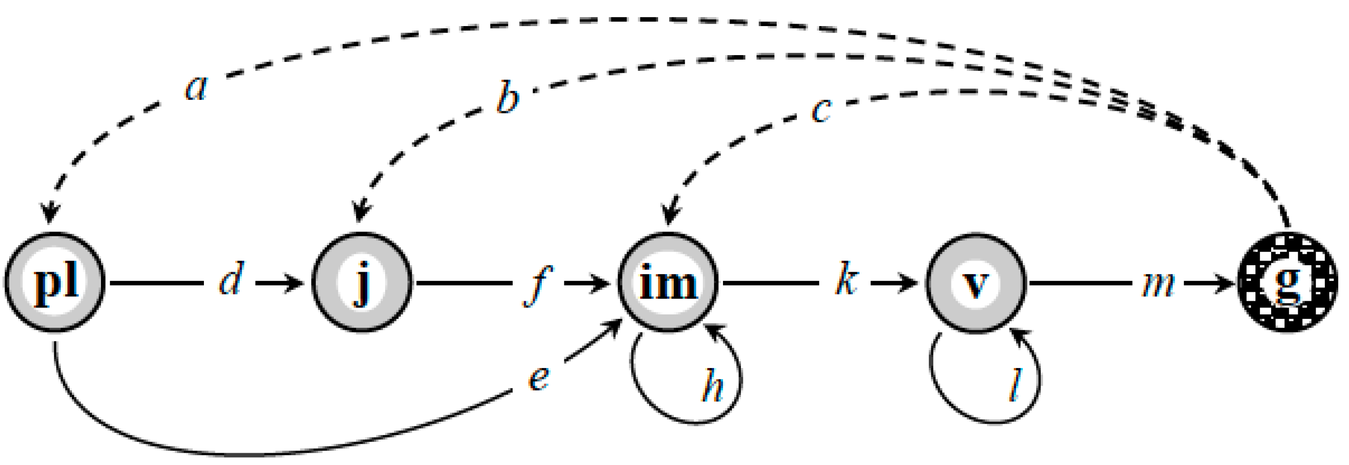
delays $\circlearrowleft$ in stages im and v, which can be explained by the fact that the harsh conditions of the highlands force the plants to resort to the “space-holder strategy” [30], i.e., staying or growing in one place for as long as possible. Poor soil quality also results in some virginal plants accumulating resources for fruiting longer than one year [30,31,32,33,34];

-

accelerated transitions as a manifestation of polyvariant ontogeny in A. albana under the alpine belt conditions in South-Western Caucasus.

The monocarpic species has only one reproductive event in its life history, and the population recruitment can be observed at each of the three stages pl, j, or im, at the moment of next census. The parameters a, b and c are accordingly the average numbers of recruiting individuals (per generative plant) found at the corresponding stage by the next census [35].

The population vector, x(t) ∈ ${ℝ}_{+}^n$, consists of 5 components:

x(t) = [pl(t), j(t), im(t), v(t), g(t)]^T, t = 2009, 2010, …, 2019,

(3)

observed on permanent sample plots in Teberda State Nature Biosphere Reserve (North-West Caucasus) and censused once a year (early August) [28] during 11 successive years (

Table 1. Structure of the local A. albana population according to observation data (Table 1 in [36]).

Stage	Stage Group Sizes (in Absolute Numbers) at the Year of Observation
	2009	2010	2011	2012	2013	2014	2015	2016	2017	2018	2019
pl	37	30	19	49	19	16	4	10	3	12	13
j	110	48	45	86	137	98	19	29	8	23	38
im	99	55	43	87	95	34	10	13	4	13	2
v	35	26	57	58	73	50	20	16	18	23	23
g	13	1	1	4	6	3	4	2	1	2	1

).

The observation data gained at each pair of successive years, t and t + 1, enabled us to calibrate the annual PPM, L(t), in a unique way to obey System (2) for t = 2009, …, 2018 (

Table 2. A. albana population projection matrices (PPMs) calibrated from 2009–2019 data, their dominant eigenvalues, and the corresponding eigenvectors (Table 3 in [36]).

Census Year, t	Matrix L(t): t → t + 1	λ1(L(t))	Vector x*, %
2009	$\left[\begin{array}{ccccc}0& 0& 0& 0& \raisebox{1ex}{$30$}\!\left/ \!\raisebox{-1ex}{$13$}\right.\\ \raisebox{1ex}{$8$}\!\left/ \!\raisebox{-1ex}{$37$}\right.& 0& 0& 0& \raisebox{1ex}{$40$}\!\left/ \!\raisebox{-1ex}{$13$}\right.\\ \raisebox{1ex}{$2$}\!\left/ \!\raisebox{-1ex}{$37$}\right.& \raisebox{1ex}{$22$}\!\left/ \!\raisebox{-1ex}{$110$}\right.& \raisebox{1ex}{$28$}\!\left/ \!\raisebox{-1ex}{$99$}\right.& 0& \raisebox{1ex}{$3$}\!\left/ \!\raisebox{-1ex}{$13$}\right.\\ 0& 0& \raisebox{1ex}{$7$}\!\left/ \!\raisebox{-1ex}{$99$}\right.& \raisebox{1ex}{$19$}\!\left/ \!\raisebox{-1ex}{$35$}\right.& 0\\ 0& 0& 0& \raisebox{1ex}{$1$}\!\left/ \!\raisebox{-1ex}{$35$}\right.& 0\end{array}\right]$	0.5661	$\left[\begin{array}{c}10.61\\ 18.20\\ 16.99\\ 51.59\\ 2.60\end{array}\right]$
2010	$\left[\begin{array}{ccccc}0& 0& 0& 0& \raisebox{1ex}{$19$}\!\left/ \!\raisebox{-1ex}{$1$}\right.\\ \raisebox{1ex}{$14$}\!\left/ \!\raisebox{-1ex}{$30$}\right.& 0& 0& 0& \raisebox{1ex}{$31$}\!\left/ \!\raisebox{-1ex}{$1$}\right.\\ \raisebox{1ex}{$4$}\!\left/ \!\raisebox{-1ex}{$30$}\right.& \raisebox{1ex}{$22$}\!\left/ \!\raisebox{-1ex}{$48$}\right.& \raisebox{1ex}{$17$}\!\left/ \!\raisebox{-1ex}{$55$}\right.& 0& \raisebox{1ex}{$0$}\!\left/ \!\raisebox{-1ex}{$1$}\right.\\ 0& 0& \raisebox{1ex}{$34$}\!\left/ \!\raisebox{-1ex}{$55$}\right.& \raisebox{1ex}{$23$}\!\left/ \!\raisebox{-1ex}{$26$}\right.& 0\\ 0& 0& 0& \raisebox{1ex}{$1$}\!\left/ \!\raisebox{-1ex}{$26$}\right.& 0\end{array}\right]$	1.2283	$\left[\begin{array}{c}15.90\\ 31.99\\ 18.25\\ 32.83\\ 1.03\end{array}\right]$
2011	$\left[\begin{array}{ccccc}0& 0& 0& 0& \raisebox{1ex}{$49$}\!\left/ \!\raisebox{-1ex}{$1$}\right.\\ \raisebox{1ex}{$1$}\!\left/ \!\raisebox{-1ex}{$19$}\right.& 0& 0& 0& \raisebox{1ex}{$85$}\!\left/ \!\raisebox{-1ex}{$1$}\right.\\ \raisebox{1ex}{$6$}\!\left/ \!\raisebox{-1ex}{$19$}\right.& \raisebox{1ex}{$35$}\!\left/ \!\raisebox{-1ex}{$45$}\right.& \raisebox{1ex}{$21$}\!\left/ \!\raisebox{-1ex}{$43$}\right.& 0& \raisebox{1ex}{$25$}\!\left/ \!\raisebox{-1ex}{$1$}\right.\\ 0& 0& \raisebox{1ex}{$10$}\!\left/ \!\raisebox{-1ex}{$43$}\right.& \raisebox{1ex}{$48$}\!\left/ \!\raisebox{-1ex}{$57$}\right.& 0\\ 0& 0& 0& \raisebox{1ex}{$4$}\!\left/ \!\raisebox{-1ex}{$57$}\right.& 0\end{array}\right]$	1.5779	$\left[\begin{array}{c}17.20\\ 30.40\\ 39.39\\ 12.45\\ 0.55\end{array}\right]$
2012	$\left[\begin{array}{ccccc}0& 0& 0& 0& \raisebox{1ex}{$19$}\!\left/ \!\raisebox{-1ex}{$4$}\right.\\ \raisebox{1ex}{$1$}\!\left/ \!\raisebox{-1ex}{$49$}\right.& 0& 0& 0& \raisebox{1ex}{$136$}\!\left/ \!\raisebox{-1ex}{$4$}\right.\\ \raisebox{1ex}{$10$}\!\left/ \!\raisebox{-1ex}{$49$}\right.& \raisebox{1ex}{$45$}\!\left/ \!\raisebox{-1ex}{$86$}\right.& \raisebox{1ex}{$39$}\!\left/ \!\raisebox{-1ex}{$87$}\right.& 0& \raisebox{1ex}{$1$}\!\left/ \!\raisebox{-1ex}{$4$}\right.\\ 0& 0& \raisebox{1ex}{$28$}\!\left/ \!\raisebox{-1ex}{$87$}\right.& \raisebox{1ex}{$45$}\!\left/ \!\raisebox{-1ex}{$58$}\right.& 0\\ 0& 0& 0& \raisebox{1ex}{$6$}\!\left/ \!\raisebox{-1ex}{$58$}\right.& 0\end{array}\right]$	1.2641	$\left[\begin{array}{c}6.01\\ 43.15\\ 29.67\\ 19.56\\ 1.60\end{array}\right]$
2013	$\left[\begin{array}{ccccc}0& 0& 0& 0& \raisebox{1ex}{$16$}\!\left/ \!\raisebox{-1ex}{$6$}\right.\\ 0& 0& 0& 0& \raisebox{1ex}{$98$}\!\left/ \!\raisebox{-1ex}{$6$}\right.\\ \raisebox{1ex}{$2$}\!\left/ \!\raisebox{-1ex}{$19$}\right.& \raisebox{1ex}{$16$}\!\left/ \!\raisebox{-1ex}{$137$}\right.& \raisebox{1ex}{$14$}\!\left/ \!\raisebox{-1ex}{$95$}\right.& 0& \raisebox{1ex}{$2$}\!\left/ \!\raisebox{-1ex}{$6$}\right.\\ 0& 0& \raisebox{1ex}{$6$}\!\left/ \!\raisebox{-1ex}{$95$}\right.& \raisebox{1ex}{$44$}\!\left/ \!\raisebox{-1ex}{$73$}\right.& 0\\ 0& 0& 0& \raisebox{1ex}{$3$}\!\left/ \!\raisebox{-1ex}{$73$}\right.& 0\end{array}\right]$	0.6345	$\left[\begin{array}{c}7.76\\ 47.54\\ 14.34\\ 28.51\\ 1.85\end{array}\right]$
2014	$\left[\begin{array}{ccccc}0& 0& 0& 0& \raisebox{1ex}{$4$}\!\left/ \!\raisebox{-1ex}{$3$}\right.\\ 0& 0& 0& 0& \raisebox{1ex}{$19$}\!\left/ \!\raisebox{-1ex}{$3$}\right.\\ \raisebox{1ex}{$2$}\!\left/ \!\raisebox{-1ex}{$16$}\right.& \raisebox{1ex}{$2$}\!\left/ \!\raisebox{-1ex}{$98$}\right.& \raisebox{1ex}{$6$}\!\left/ \!\raisebox{-1ex}{$34$}\right.& 0& \raisebox{1ex}{$0$}\!\left/ \!\raisebox{-1ex}{$3$}\right.\\ 0& 0& \raisebox{1ex}{$4$}\!\left/ \!\raisebox{-1ex}{$34$}\right.& \raisebox{1ex}{$16$}\!\left/ \!\raisebox{-1ex}{$50$}\right.& 0\\ 0& 0& 0& \raisebox{1ex}{$4$}\!\left/ \!\raisebox{-1ex}{$50$}\right.& 0\end{array}\right]$	0.3988	$\left[\begin{array}{c}11.71\\ 56.64\\ 11.69\\ 17.46\\ 3.50\end{array}\right]$
2015	$\left[\begin{array}{ccccc}0& 0& 0& 0& \raisebox{1ex}{$10$}\!\left/ \!\raisebox{-1ex}{$4$}\right.\\ 0& 0& 0& 0& \raisebox{1ex}{$29$}\!\left/ \!\raisebox{-1ex}{$4$}\right.\\ 0& \raisebox{1ex}{$10$}\!\left/ \!\raisebox{-1ex}{$19$}\right.& \raisebox{1ex}{$3$}\!\left/ \!\raisebox{-1ex}{$10$}\right.& 0& \raisebox{1ex}{$0$}\!\left/ \!\raisebox{-1ex}{$4$}\right.\\ 0& 0& \raisebox{1ex}{$5$}\!\left/ \!\raisebox{-1ex}{$10$}\right.& \raisebox{1ex}{$17$}\!\left/ \!\raisebox{-1ex}{$20$}\right.& 0\\ 0& 0& 0& \raisebox{1ex}{$2$}\!\left/ \!\raisebox{-1ex}{$20$}\right.& 0\end{array}\right]$	1.0679	$\left[\begin{array}{c}9.19\\ 26.66\\ 18.28\\ 41.94\\ 3.93\end{array}\right]$
2016	$\left[\begin{array}{ccccc}0& 0& 0& 0& \raisebox{1ex}{$3$}\!\left/ \!\raisebox{-1ex}{$2$}\right.\\ 0& 0& 0& 0& \raisebox{1ex}{$8$}\!\left/ \!\raisebox{-1ex}{$2$}\right.\\ \raisebox{1ex}{$2$}\!\left/ \!\raisebox{-1ex}{$10$}\right.& \raisebox{1ex}{$5$}\!\left/ \!\raisebox{-1ex}{$29$}\right.& \raisebox{1ex}{$5$}\!\left/ \!\raisebox{-1ex}{$13$}\right.& 0& \raisebox{1ex}{$0$}\!\left/ \!\raisebox{-1ex}{$2$}\right.\\ 0& 0& \raisebox{1ex}{$8$}\!\left/ \!\raisebox{-1ex}{$13$}\right.& \raisebox{1ex}{$20$}\!\left/ \!\raisebox{-1ex}{$22$}\right.& 0\\ 0& 0& 0& \raisebox{1ex}{$1$}\!\left/ \!\raisebox{-1ex}{$22$}\right.& 0\end{array}\right]$	0. 9611	$\left[\begin{array}{c}5.26\\ 14.04\\ 6.02\\ 71.30\\ 3.37\end{array}\right]$
2017	$\left[\begin{array}{ccccc}0& 0& 0& 0& \raisebox{1ex}{$12$}\!\left/ \!\raisebox{-1ex}{$1$}\right.\\ 0& 0& 0& 0& \raisebox{1ex}{$23$}\!\left/ \!\raisebox{-1ex}{$1$}\right.\\ \raisebox{1ex}{$3$}\!\left/ \!\raisebox{-1ex}{$3$}\right.& \raisebox{1ex}{$2$}\!\left/ \!\raisebox{-1ex}{$8$}\right.& \raisebox{1ex}{$8$}\!\left/ \!\raisebox{-1ex}{$12$}\right.& 0& \raisebox{1ex}{$0$}\!\left/ \!\raisebox{-1ex}{$1$}\right.\\ 0& 0& \raisebox{1ex}{$2$}\!\left/ \!\raisebox{-1ex}{$12$}\right.& \raisebox{1ex}{$21$}\!\left/ \!\raisebox{-1ex}{$28$}\right.& 0\\ 0& 0& 0& \raisebox{1ex}{$2$}\!\left/ \!\raisebox{-1ex}{$28$}\right.& 0\end{array}\right]$	1.1206	$\left[\begin{array}{c}12.93\\ 24.78\\ 42.13\\ 18.95\\ 1.21\end{array}\right]$
2018	$\left[\begin{array}{ccccc}0& 0& 0& 0& \raisebox{1ex}{$13$}\!\left/ \!\raisebox{-1ex}{$2$}\right.\\ 0& 0& 0& 0& \raisebox{1ex}{$38$}\!\left/ \!\raisebox{-1ex}{$2$}\right.\\ \raisebox{1ex}{$1$}\!\left/ \!\raisebox{-1ex}{$12$}\right.& \raisebox{1ex}{$1$}\!\left/ \!\raisebox{-1ex}{$23$}\right.& \raisebox{1ex}{$0$}\!\left/ \!\raisebox{-1ex}{$13$}\right.& 0& \raisebox{1ex}{$0$}\!\left/ \!\raisebox{-1ex}{$2$}\right.\\ 0& 0& \raisebox{1ex}{$1$}\!\left/ \!\raisebox{-1ex}{$13$}\right.& \raisebox{1ex}{$22$}\!\left/ \!\raisebox{-1ex}{$23$}\right.& 0\\ 0& 0& 0& \raisebox{1ex}{$1$}\!\left/ \!\raisebox{-1ex}{$23$}\right.& 0\end{array}\right]$	0.9617	$\left[\begin{array}{c}13.22\\ 38.66\\ 2.89\\ 43.27\\ 1.96\end{array}\right]$

). Note that these 10 PPMs differ drastically from one another, with their λ₁s being either markedly greater or less than 1. This means that variations in the environment from year to year do affect the germination and growth of A. albana plants.

2.2. Local Meteodata, Statistical Treatment

In addition to monitoring the local population of A. albana, also monitored were climatic parameters at the site (an alpine heath), close to the permanent plots of the population under study. From a variety of meteorological data on the air and soil registered by the local temperature/ humidity sensors, we selected certain key environmental factors effecting the population status and development, i.e., seed germination, and seedling survival and growth, under severe conditions of the alpine belt. Twenty-one parameters were selected: the minimal, maximal, and average air temperatures in the previous-year autumn (September–October) and current-year spring plus early summer period (May–June); the soil surface and 10-cm-depth temperatures in the previous-year autumn (September–October) and current-year spring plus early summer period (May–June) the duration of freezing on the soil surface and 10 cm depth during the winter period (the sum of the days when the maximal temperature did not exceed −1 °C from the previous-year November to the current-year April); the daily average soil moisture pressure at the 10 cm soil depth during June, 17–30. The data on meteorological and soil indicators were collected by standard methods with automatic sensors.

In addition, a weather station, the Teberda State Meteorological Station (TSMS, the Karachay-Cherkess Republic, Russian Federation), is located in a mountain valley (43.45° N, 41.73° E) 5 km from the alpine plots. We developed a database of 13 years (2007–2019) of observations at the TSMS accounting for 15 climatic indicators, which might demonstrate statistical relationships with the status and growth of the population under study. Ecologically significant climatic indicators were taken: the average, minimal and maximal temperatures in the previous-year autumn (September and October); the minimum, maximum, and average temperatures in spring (May) and early summer (June); the amount of precipitation in the previous-year fall (September and October), the current-year spring to early summer period (May and June), and the winter period (from the previous-year November to the current-year May). The TSMS collects climatic indicators according to the standard list of indicators framed by international requirements. Station staff kindly shared these data with us.

To detect a factor effecting λ₁(t), we developed multiple regression models by the least-squares method (ordinary least squares, OLS). Because the number of analyzed factors significantly exceeds the number of observations and only three predictors at most could be included in the model, they were selected by stepwise regression (forward regression). Before the analysis, all of the factors were checked for correlations, so as not to include factors correlated with each other in one model. The distribution of λ₁(t), a dependent variable, corresponds to the normal distribution (p = 0.793 in the Shapiro–Wilk test [37]). Whether the errors are normally distributed was visually assessed on the quantile–quantile plots.

Because λ₁(t) was calculated annually, this variable can be considered a time series, so we checked the best models for autocorrelations. To do this, we built two generalized linear models (function gls of the nlme package in the statistical environment R [38]) with and without level-1 autocorrelation (AR1) and compared them with each other using the log-likelihood ratio (anova function in R [39]). It was found that autocorrelations did not make any significant contributions and were therefore not included in the final models.

As a result, the study allows us to conclude that the λ₁(t) variable depends positively on the minimum air temperatures in May–June in the alpine heath; this was found to be the only significant predictor in the models with one factor included. The best multiple regression model explained 99% of the variance and included three factors: minimum air temperatures in May–June, precipitation from November to May, and maximum 10-cm-depth soil temperatures in May–June (Supplementary Material). The λ₁(t) variable increases with increasing temperatures and decreasing precipitation. We revealed the highest significance of relationships between λ₁(t) and weather factors (registered at the TSMS) in the models including the precipitation from November to May and the minimum temperatures from May to June (p < 0.1). However, the temperature time series had certain gaps, so that only the time series of the November-to-May precipitation sum, Pr(t), was selected for the further study.

2.3. Revealing the Pattern of Transition Matrix and Estimating Its Elements

We construct a Markov chain formalism in which the element p_ij of the transition matrix, P = [p_ij], is a probability of the j to i transition, i.e., matrix P is column-stochastic [40]. For example, if we consider the sequence of given annual PPM as a realization of a Markov chain, then we see the chronological 10-year sequence: L(2009), …, L(2018) (Table 2). If this short-term sequence is repeated periodically in the long term, the transition matrix of the corresponding Markov chain would then have the following 10 × 10 pattern:

$$\mathit{P}=\left[\begin{array}{ccccc}0& 0& \dots & 0& 1\\ 1& 0& \dots & 0& 0\\ 0& 1& \dots & 0& 0\\ ⋮& ⋮& ⋮& ⋮& ⋮\\ 0& 0& \dots & 1& 0\end{array}\right],$$

The chain thus becomes a deterministic, rather than a stochastic, process.

To obtain a longer-than-10 stochastic sequence of PPMs, we identify each of the 10 given PPMs, L(t), t = 2009, …, 2018, with the value of precipitation sum, Pr(t), during the corresponding, t → t + 1, period (see Section 2.2). All of these values are different, and we call them reference values, numbered from 1 to 10 in chronological order. Fortunately, precipitations have been measured in the TSMS since 1960, providing a 59-point time series. The task is thereafter to associate each successive point, Pr(k), k = 1960, …, 2018, of that series to one of the 10 reference values, which was done using the absolute difference, |Pr(k) − Pr(t)|, as a measure of distance, selecting the closest reference point:

$$t_{\mathrm{next}}=t\in \{2009,\dots ,2018\}||Pr(k)-Pr(t)|=\underset{t}{\min }|Pr(k)-Pr(t)|.$$

(4)

Because the reference values are different, we obtain, in a unique way, a 59-member sequence of year labels “t” (t = 2009, …, 2018) where every next label represents a particular transition event and the last 9 labels only represent the course of time. The total sequence enables identifying all possible types of transition occurring in the sequence and representing them as a directed graph (digraph, [3]) of transitions between 10 nodes identified with the reference years. The nine successive transitions 2009 → 2010 → … → 2018 should constitute an evident subgraph of the total digraph. Counting the number of times a particular label transits to itself or another specific label, we obtain the frequency of this transition to be considered as the corresponding transition probability.

For instance, to obtain the value of p₁₂ we find first how many times label ”2010” occurs among the 59 labels (8 times, in fact), then count how many of all ”2010”s in the sequence are followed by “2009” (i.e., “2009” occurs immediately after “2010”; 1 time, in fact); the fraction of the latter by the former (1/8) gives therefore the frequency needed. Inspecting all of the remaining potential “followers” in this way, we obtain all remaining elements of the 2nd column in P. The nonzero values of these generate all the digraph arcs outgoing from the “2010” node. Repeating this step for each column of P results both in the completed digraph (matrix pattern) and the column-stochastic matrix itself.

Once the transition matrix, P, has been found, its dominant eigenvector is calculated in a routine way. When normalized to be stochastic, this vector gives the steady-state distribution, ss*, of the chain states [40], and can be used in iid MC simulations (ss* iid) instead of the uniform distribution (equiprobable states).

2.4. Estimating λ_S by the Direct MC Method with a Markov Chain

Once the transition matrix, P = [p_ij], has been found, it allows MC experiments in which the sequence of PPMs follows a realization of the corresponding Markov chain that has a given finite length, long enough to reveal the convergence in the Sequence (2). To ensure that the random sequences are reproducible in computer experiments, we begin each realization with the same initial population vector, x(τ = 0) = x(2009) (Table 1) and the same PPM, L₀ = L(2009) (Table 2), albeit the limit does not depend on this choice [9,10,11,12].

Then, the first column of P, equal to [p₁₁, p₂₁, _…, p_10,1]^T, gives the finite probability distribution for the next state, i, of the chain (a row number in this column) and, hence, for the next annual PPM to be chosen. This is equivalent to tossing an imperfect 10-face dice with unequal face probabilities, some of which may be zero in accordance with the pattern of P to be revealed. Face i gives the number of next column, [p_1i, p_2i, _…, p_10,i]^T, thus defining the dice to be tossed. This is the basic step of our MC simulations, and Appendix A illustrates how efficiently it can be implemented in MATLAB.

Note that the iid choice represents a particular case of the Markov chain choice when the transition matrix P consists of 10 identical columns giving the desired distribution, hence the dice becoming perfect when the distribution is uniform. This enables us to use the same computer program for simulating both nontrivial Markov chain sequences and the iid ones.

3. Results

3.1. The Pattern of P = [p_ij] and the Estimates of p_ij

Following the procedure introduced in Section 2.3, we revealed a pattern of transitions among the Markov chain states associated with the 10 known annual PPMs, L(t), t = 2009, …, 2018 (Figure 3).

Although appearing to be entangled, the graph is not trivially complete: some transitions have not been observed, and hence are not presented here. Clearly observed are the chronological successive transitions from 2009 to 2018, shown as the straightforward green arrows in the figure. In addition to a small number of backward curvilinear arrows, they clearly ensure the graph is strongly connected, i.e., for any pair of nodes there exists a finite directed path from one node to the other [3]. This means matrix P is irreducible [4] and, hence, the Markov chain is regular [40], containing the sole ergodic set of all 10 states; thus, Limit (2) exists when the random choice of PPMs is governed by this Markov chain.

The elements of transition matrix, P = [p_ij], of this chain are obtained as the frequencies of the corresponding transitions revealed by means of the procedure introduced in Section 2.3 (

Table 3. Transition matrix of the Markov chain governing the random choice of annual PPMs and its dominant stochastic eigenvector.

Incoming States	Outgoing States										Eigenvector, ss*
	2009	2010	2011	2012	2013	2014	2015	2016	2017	2018
2009	0	1/8	0	1/9	0	0	0	0	0	0	0.0359
2010	1/2	1/4	0	1/9	1/3	0	0	1/9	0	1/3	0.1437
2011	0	1/4	0	0	0	0	0	0	1/2	0	0.0359
2012	0	0	1/2	1/9	1/3	1/4	0	0	0	1/3	0.1613
2013	0	0	0	1/9	0	1/8	1/7	0	0	0	0.0519
2014	0	1/8	1/2	1/9	1/3	0	2/7	1/9	0	1/6	0.1389
2015	0	1/8	0	1/9	0	1/8	0	1/3	0	1/6	0.1164
2016	1/2	0	0	0	0	1/4	2/7	1/3	0	0	0.1289
2017	0	0	0	1/9	0	1/8	0	1/9	1/4	0	0.0661
2018	0	1/8	0	2/9	0	1/8	2/7	0	1/4	0	0.1210
Column Sum	1	1	1	1	1	1	1	1	1	1	1

). The last column of Table 3 shows the steady-state distribution of chain states (given by ss*, the dominant stochastic eigenvalue of P).

3.2. Estimates of λ_S

Each realization of the finite random sequence from Definition (2) generates its own value of the λ_S estimate. (An algorithm to calculate the final term of the sequence, then to obtain an estimate, is presented in Appendix B). Several realizations generate a set of estimates, with their minimal and maximal values, and hence a range of estimates. The length of the finite sequence and the number of times it has to be constructed constitute a design of MC experiments to estimate the λ_S for a given set of annual PPMs. The longer the sequence, the closer its final term to the limit value. The greater the number of random realizations, the wider should be the range of estimates ensuing from the set.

We apply the same design of simulation experiments as before (Table 6 in [13]) plus two more options for comparison of the results. (The algorithm to repeat construction of the sequence of a given length and to obtain the range of estimates is presented in Appendix C).

The figures shown in

Table 4. Estimating the stochastic growth rate, λ_S, of the local A. albana population by the direct Monte Carlo technique.

Product “Length” 1	Number of Realizations	Range of Variations in the Estimates of λS; Range Length in the Following Series:
		Markov Chain	Equiprobable iid	ss* iid
1 × 105	13	[0.924332, 0.928207]; 0.003876	[0.935773, 0.939521]; 0.003749	[0.940098, 0.945336]; 0.005237
	33	[0.924332, 0.928207]; 0.003876	[0.933281, 0.939521]; 0.006240	[0.939897, 0.945336]; 0.005439
	100	[0.923628, 0.928371]; 0.004743	[0.933281, 0.940469]; 0.007188	[0.939383, 0.945336]; 0.005953
2 × 105	13	[0.925053, 0.927760]; 0.002707	[0.935810, 0.938245]; 0.002434	[0.940534, 0.943727]; 0.003193
	33	[0.924339, 0.927760]; 0.003420	[0.935694, 0.93465]; 0.002770	[0.940534, 0.943727]; 0.003193
	100	[0.924046, 0.927760]; 0.003714	[0.935120, 0.939514]; 0.004394	[0.940331, 0.943907]; 0.003571
3 × 105	13	[0.925153, 0.927434]; 0.002281	[0.935323, 0.938044]; 0.002721	[0.940505, 0.942882]; 0.002377
	33	[0.924483, 0.927434]; 0.002950	[0.935323, 0.938272]; 0.002949	[0.940505, 0.942919]; 0.002415
	100	[0.924483, 0.927434]; 0.002950	[0.934746, 0.938613]; 0.003867	[0.939569, 0.943653]; 0.004084
5 × 105	13	[0.924771, 0.926431]; 0.001660	[0.936047, 0.937644]; 0.001597	[0.941309, 0.942485]; 0.001176
	33	[0.924771, 0.926558]; 0.001787	[0.936047, 0.937886]; 0.001838	[0.941043, 0.943080]; 0.002037
	100	[0.924714, 0.926724; 0.002009	[0.935679, 0.938194]; 0.002515	[0.941012, 0.943089]; 0.002077
1 × 106	13	[0. 925045, 0.925313]; 0.000676	[0.936453, 0.937261]; 0.000807	[0.941301, 0.942233]; 0.000933
	33	[0. 925045, 0.926010]; 0.000965	[0.936453, 0.937261]; 0.000808	[0.941301, 0.942275]; 0.000974
	100	[0.925045, 0.926048]; 0.001003	[0.936341, 0.937473]; 0.001133	[0.941218, 0.942491]; 0.001273
	1000	[0.924874, 0.926079]; 0.001205	[0.936297, 0.937635]; 0.001339	[0.941195, 0.942521]; 0.001326

¹ The number of a finite member of the sequence {N(τ)} that approximates its limit (2) as τ → ∞; this coincides with the number of cofactors in the product of randomly chosen matrices L_τ–1 L_τ–2 … L₁ L₀ that still retains vector x(τ) from becoming the computer zero due to normalizing, at each step, by coef = 0.936979, a specially selected “scaling factor”; greater detail is provided in [41].

confirm our expectations described above (see the digits in bold). In this regard, one thousand repetitions of the one-million-long sequence in the Markov chain series generate the most reliable range of λ_S estimates, and this range has an order of 10⁻³. Other series generate consistently greater estimates and the markedly wider ranges of estimates as was expected (see Section 1). Unfortunately, the first decimal digit only obtained in the iid estimates can be trusted.

4. Discussion

The LCG for the stage-structured population of A. albana (Figure 2) deliberately does not contain the stage of dormant seeds. The motivation for this was provided in the original case study [28] and repeated here in Section 2.1. In fact, the dormant seeds represent one of the “cryptic life stages” ([42], p.1), and one of the ‘’persistent problems in the construction of matrix population models” ([43], p.1). It has recently become a subject of extensive discussion [42,43,44], yet without any definite conclusion that the seed stage is necessary in a model. Moreover, a deeper investigation of the A. albana model with the seed stage incorporated within certain botanical bounds for uncertain seed-related parameters [29] revealed that it cannot principally change the qualitative outcome of the “no-seeds” model.

The expectations of how the ranges of the stochastic growth rate depend on the length of the finite sequence and the number of realizations were both prompted by a tenet of real analysis, in addition to common sense and our observations from our former MC experiments (Table 6 in [13]). However, it was only a hypothesis that “Realistic choice of annual matrices contracts the range of λ_S estimates” as compared to the iid choice. This hypothesis is now confirmed with the evident proof in Table 4: every line, excepting those with the smallest number (13) of realizations, confirms the point. Thus, the outcome of this comparison is not surprising to the authors.

The unexpected finding is that the ss* iid experiments always yield worse estimates than the equiprobable iid series (cf. the 4th and 5th columns), despite the former being strongly related to the Markov chain (the steady-state distribution). Moreover, these figures indicate our corresponding hypothesis (see the last paragraph of Section 1) is unfounded. Indeed, the “hypothesis” was rejected by experts [45] who studied population dynamics under environmental variability [21,45,46,47], with an argument that the ss* iid choices ignore the transient dynamics and possible autocorrelations.

Regarding the absolute values of the λ_S estimates obtained from 10 annual PPMs (Table 2), these are markedly greater than those obtained from eight PPMs (Table 6 in [13], the difference is in the order of 10⁻¹) and correspondingly closer to 1. A clear reason is that λ₁ of the 9th ppm is clearly greater than 1, while the 10th λ₁, although less than 1, is close to 1 (Table 2). However, the 10-year estimates of λ_S are still less than 1, implying an unfavorable forecast of the species viability in this habitat in the long term. This confirms the Red-Book classification of A. albana [25,26], although the classification is traditionally based on field observations and expert assessments rather than any quantitative measures ensuing from the population models.

Comparing the values obtained under the “realistic choice” to those in the iid series, we reveal the former to be markedly lower (Table 2). This means that less favorable environments occurred in the long time series of observations much more frequently than would be the case under the independent permanent probability distributions. If a model is a kind of caricature of reality, then the governing Markov chain calibrated from real weather data represents a step forward, from the crude iid to a softer image of reality. As a method that provides more accurate estimates of λ_S, it can be recommended for the application to any discrete-structured population case study with multi-year data combined with weather observations.

It may seem at first glance that, in our Markov chain simulations, we have used the well-known MCMC method (Markov Chain Monte Carlo). However, our method is original: although the classical MCMC searches for “an ergodic Markov chain whose stationary distribution is f ” ([48], p. 268) (ss* in our notation), a given steady-state distribution of its state probabilities, we build a chain by analyzing its long (59-year) realization in a vast array of local meteorological data and obtain ss* in a routine way from the transition matrix.

5. Conclusions

Given a finite set of annual PPMs signifying the variable environment of a local population, the stochastic growth rate, λ_S, can be approximated, in accordance with its definition as a certain limit of the time-averaged population size, from a finite sequence of PPMs chosen randomly from the set for each successive term of the sequence. The rule of the random choice should conform with real variations in key factors of the environment, and a governing Markov chain represents a step forward in this direction. Once the transition matrix of the chain has been constructed and calibrated from real observation data, it can govern the choice in a series of Monte Carlo simulations to result in a certain range of λ_S estimates. The greater the number of random realizations in a series, the wider is the range. However, the longer the sequence, the closer the estimate approaches to the limit.

The main conclusion concerning the range of λ_S estimates is given in the title of this paper, compared to the iid rule of the random choice, which is a simple artificial construction popular in the literature. In our case study, the “realistic choice” results in a range of 10⁻³ order of magnitude, while the actual value of λ_S is markedly less than those obtained in the iid estimates. Therefore, only their first decimal digits can be trusted in the absence of the governing Markov chain. The absolute value of λ_S in the range of [0.924874, 0.926079] means that the local Androsace albana population may decrease by more than half in 10 years under the observed conditions. This confirms the current Red-Book classification of the species [25,26] as Near Threatened, albeit the findings indicate it is even more “Threatened” than previously indicated by the iid method, witnessing the urgent need to further monitor the population of this rare endemic species.

References

1. Caswell, H. Matrix Population Models: Construction, Analysis and Interpretation, 2nd ed.; Sinauer Associates: Sunderland, MA, USA, 2001. [Google Scholar]
2. Logofet, D.O. Projection matrices revisited: A potential-growth indicator and the merit of indication. J. Math. Sci. 2013, 193, 671–686. [Google Scholar] [CrossRef]
3. Harary, F.; Norman, R.Z.; Cartwright, D. Structural Models: An Introduction to the Theory of Directed Graphs; John Wiley: New York, NY, USA, 1965. [Google Scholar]
4. Horn, R.A.; Johnson, C.R. Matrix Analysis; Cambridge University Press: Cambridge, UK, 1990. [Google Scholar]
5. Logofet, D.O. Matrices and Graphs: Stability Problems in Mathematical Ecology; CRC Press: Boca Raton, FL, USA, 1993. [Google Scholar]
6. Gantmacher, F.R. Matrix Theory; Chelsea Publ.: New York, NY, USA, 1959. [Google Scholar]
7. Logofet, D.O.; Ulanova, N.G.; Belova, I.N. Adaptation on the ground and beneath: Does the local population maximize its λ1? Ecol. Complex. 2014, 20, 176–184. [Google Scholar] [CrossRef]
8. Logofet, D.O. Projection matrices in variable environments: λ1 in theory and practice. Ecol. Model. 2013, 251, 307–311. [Google Scholar] [CrossRef]
9. Furstenberg, H.; Kesten, H. Products of random matrices. Ann. Math. Stat. 1960, 31, 457–469. [Google Scholar] [CrossRef]
10. Oseledec, V.I. A multiplicative ergodic theorem: Ljapunov characteristic numbers for dynamical systems. Trans. Mosc. Math. Soc. 1968, 19, 197–231. [Google Scholar]
11. Cohen, J.E. Ergodicity of age structure in populations with Markovian vital rates, I: Countable states. J. Amer. Stat. Ass. 1976, 71, 335–339. [Google Scholar] [CrossRef]
12. Tuljapurkar, S.D. Population Dynamics in Variable Environments; Springer: New York, NY, USA, 1990. [Google Scholar]
13. Logofet, D.O. Does averaging overestimate or underestimate population growth? It depends. Ecol. Model. 2019, 411, 108744. [Google Scholar] [CrossRef]
14. Richardson, C.W. Stochastic simulation of daily precipitation, temperature and solar radiation. Water Resour. Res. 1981, 17, 182–190. [Google Scholar] [CrossRef]
15. Johnson, G.L.; Hanson, C.L.; Hardegree, S.P.; Ballard, E.B. Stochastic weather simulation—Overview and analysis of two commonly used models. J. Appl. Meteorol. 1996, 35, 1878–1896. [Google Scholar] [CrossRef] [Green Version]
16. Johnson, G.L.; Daly, C.; Taylor, G.H.; Hanson, C.L. Spatial variability and interpolation of stochastic weather simulation model parameters. J. Appl. Meteorol. 2000, 39, 778–796. [Google Scholar] [CrossRef]
17. Dubrovsky, M.; Zalud, Z.; Stastna, M. Sensitivity of CERES–Maize yields to statistical structure of daily weather series. Clim. Chang. 2000, 46, 447–472. [Google Scholar] [CrossRef]
18. Cohen, J.E. Ergodicity of age structure in populations with Markovian vital rates, II: General states. Adv. Appl. Probab. 1977, 9, 18–37. [Google Scholar] [CrossRef]
19. Steinsaltz, D.; Tuljapurkar, S.; Horvitz, C. Derivatives of the stochastic growth rate. Theor. Popul. Biol. 2011, 80, 1–15. [Google Scholar] [CrossRef] [PubMed] [Green Version]
20. Sanz, L. Conditions for growth and extinction in matrix models with environmental stochasticity. Ecol. Model. 2019, 411, 108797. [Google Scholar] [CrossRef]
21. Morris, W.F.; Tuljapurkar, S.; Haridas, C.V.; Menges, E.S.; Horvitz, C.C.; Pfister, C.A. Sensitivity of the population growth rate to demographic variability within and between phases of the disturbance cycle. Ecol. Lett. 2006, 9, 1331–1341. [Google Scholar] [CrossRef]
22. Rees, M.; Ellner, S.P. Integral projection models for populations in temporally varying environments. Ecol. Monogr. 2009, 79, 575–594. [Google Scholar] [CrossRef] [Green Version]
23. Ozgul, A.; Childs, D.Z.; Oli, M.K.; Armitage, K.B.; Blumstein, D.T.; Olson, L.E.; Tuljapurkar, S.; Coulson, T. Coupled dynamics of body mass and population growth in response to environmental change. Nature 2010, 466, 482–485. [Google Scholar] [CrossRef] [Green Version]
24. Williams, H.J.; Jacquemyn, H.; Ochocki, B.M.; Brys, R.; Miller, T.E.X. Life history evolution under climate change and its influence on the population dynamics of a long-lived plant. J. Ecol. 2015, 103, 798–808. [Google Scholar] [CrossRef]
25. Red Book of the Adygea Republic: Rare and Endangered Objects of Fauna and Flora: In 2 Parts, Part 1: Plants and Fungi, 2nd ed.; Zamotaylov, A.S. (Ed.) Kachestvo: Maykop, Russia, 2012. (In Russian) [Google Scholar]
26. Red Book of the Krasnodar Territory (Plants and Mushrooms), 3nd ed.; Litvinskaya, S.A. (Ed.) Design Bureau No. 1: Krasnodar, Russia, 2017. (In Russian) [Google Scholar]
27. Kazantseva, E.S. Population Dynamics and Seed Productivity of Short-Lived Alpine Plants in the North-West Caucasus. Ph.D Thesis, Moscow State University, Moscow, Russia, 2016. (In Russian). [Google Scholar]
28. Logofet, D.O.; Kazantseva, E.S.; Belova, I.N.; Onipchenko, V.G. How long does a short-lived perennial live? A modelling approach. Biol. Bull. Rev. 2018, 8, 406–420. [Google Scholar] [CrossRef]
29. Logofet, D.O.; Kazantseva, E.S.; Belova, I.N.; Onipchenko, V.G. Local population of Eritrichium caucasicum as an object of mathematical modelling. I. Life cycle graph and a nonautonomous matrix model. Biol. Bull. Rev. 2017, 7, 415–427. [Google Scholar] [CrossRef]
30. Körner, C. Alpine Plant Life: Functional Plant Ecology of High Mountain Ecosystems, 2nd ed.; Springer: Berlin/Heidelberg, Germany, 2003. [Google Scholar]
31. Rabonov, T.A. Life cycle of perennial herbaceous plants in meadow phytocoenoses. Trudi Bot. Inst. Acad. Nauk SSSR Ser. 3. Geobot. 1950, 6, 7–204. (In Russian) [Google Scholar]
32. Rabotnov, T.A. Fitotsenologiya (Phytocenology); Moscow State Univ. Publ.: Moscow, Russia, 1978. (In Russian) [Google Scholar]
33. Bender, M.H.; Baskin, J.M.; Baskin, C.C. Age of maturity and life span in herbaceous, polycarpic perennials. Bot. Rev. 2000, 66, 311–349. [Google Scholar] [CrossRef]
34. Keller, R.; Vittoz, P. Clonal growth and demography of a hemicryptophyte alpine plant: Leontopodium alpinum Cassini. Alp. Bot. 2015, 125, 31–40. [Google Scholar] [CrossRef]
35. Logofet, D.O.; Kazantseva, E.S.; Onipchenko, V.G. Seed bank as a persistent problem in matrix population models: From uncertainty to certain bounds. Ecol. Model. 2020, 438, 109284. [Google Scholar] [CrossRef]
36. Logofet, D.O.; Kazantseva, E.S.; Belova, I.N.; Onipchenko, V.G. Backward prediction confirms the conclusion on local plant population viability. Zhurnal Obs. Biol. (J. Gen. Biol.) 2020, 81, 257–271. (In Russian) [Google Scholar] [CrossRef]
37. Shapiro, S.S.; Wilk, M.B. An analysis of variance test for normality (complete samples). Biometrika 1965, 52, 591–611. [Google Scholar] [CrossRef]
38. Pinheiro, J.; Bates, D.; DebRoy, S.; Sarkar, D.; R Core Team. nlme: Linear and Nonlinear Mixed Effects Models. R Package Version 3.1-128. Available online: http://CRAN.R-project.org/package=nlme (accessed on 20 October 2020).
39. R Core Team. R: A Language and Environment for Statistical Computing; R Foundation for Statistical Computing: Vienna, Austria, 2016; Available online: https://www.R-project.org/ (accessed on 20 October 2020).
40. Kemeny, J.G.; Snell, J.L. Finite Markov Chains; Van Nostrand: Princeton, NJ, USA, 1960. [Google Scholar]
41. Logofet, D.O.; Kazantseva, E.S.; Belova, I.N.; Onipchenko, V.G. Local population of Eritrichium caucasicum as an object of mathematical modelling. III. Population growth in the random environment. Biol. Bull. Rev. 2019, 9, 453–464. [Google Scholar] [CrossRef]
42. Nguyen, V.; Buckley, Y.M.; Salguero-Gomez, R.; Wardle, G.M. Consequences of neglecting cryptic life stages from demographic models. Ecol. Model. 2019, 408, 108723. [Google Scholar] [CrossRef]
43. Kendall, B.E.; Fujiwara, M.; Diaz-Lopez, J.; Schneider, S.; Voigt, J.; Wiesner, S. Persistent problems in the construction of matrix population models. Ecol. Model. 2019, 406, 33–43. [Google Scholar] [CrossRef]
44. Che-Castaldo, J.; Jones, O.; Kendall, B.E.; Burns, J.H.; Childs, D.Z.; Ezard, T.H.; Hernandez-Yanez, H.; Hodgson, D.J.; Jongejans, E.; Knight, T.; et al. Comments to “Persistent problems in the construction of matrix population models”. Ecol. Model. 2020, 416, 108913. [Google Scholar] [CrossRef] [Green Version]
45. Tuljapurkar, S.D.; Stanford University, Stanford, CA, USA. Personal Communication, 2020.
46. Tuljapurkar, S.D.; Haridas, C.V. Temporal autocorrelation and stochastic population growth. Ecol. Lett. 2006, 9, 327–337. [Google Scholar] [CrossRef] [PubMed]
47. Morris, W.F.; Pfister, C.A.; Tuljapurkar, S.; Haridas, C.V.; Boggs, C.L.; Boyce, M.S.; Bruna, E.M.; Church, D.R.; Coulson, T.; Doak, D.F.; et al. Longevity can buffer plant and animal populations against changing climatic variability. Ecology 2008, 89, 19–25. [Google Scholar] [CrossRef] [PubMed] [Green Version]
48. Robert, C.P.; Casella, G. Monte Carlo Statistical Methods; Springer: New York, NY, USA, 2004. [Google Scholar]
49. Mathworks Documentation. Available online: https://www.mathworks.com/help/matlab/ref/rand.html?s_tid=srchtitle (accessed on 20 October 2020).
50. Mathworks Documentation. Available online: https://www.mathworks.com/help/matlab/ref/global.html (accessed on 20 October 2020).
51. Mathworks Documentation. Available online: https://www.mathworks.com/help/matlab/ref/rng.html (accessed on 20 October 2020).
Figure 1. Ontogenetic stages of Androsace albana: pl, seedlings; j, juvenile plants; im, immature plants; v, adult vegetative plants, and g, generative plants, the stages being distinguishable in the field [28].
Mathematics 08 02252 g001
Figure 2. Life cycle graph for a local population of Androsace albana observed once per year. Ontogenetic stage notations as in Figure 1. Solid arrows indicate transitions occurring for one year (no transitions, in particular); dashed arrows correspond to annual recruitment [28].
Mathematics 08 02252 g002
Figure 3. The pattern of transitions between the weather types associated with given annual PPMs as revealed in the 59-year observations.
Mathematics 08 02252 g003