Comprehensive Review of Deep Reinforcement Learning Methods and Applications in Economics

 ,
,  ,
,  ,
,
Abstract
:1. Introduction
- Classification of the existing DL, RL, and DRL approaches in economics.
- Providing extensive insights into the accuracy and applicability of DL-, RL-, and DRL-based economic models.
- Discussing the core technologies and architecture of DRL in economic technologies.
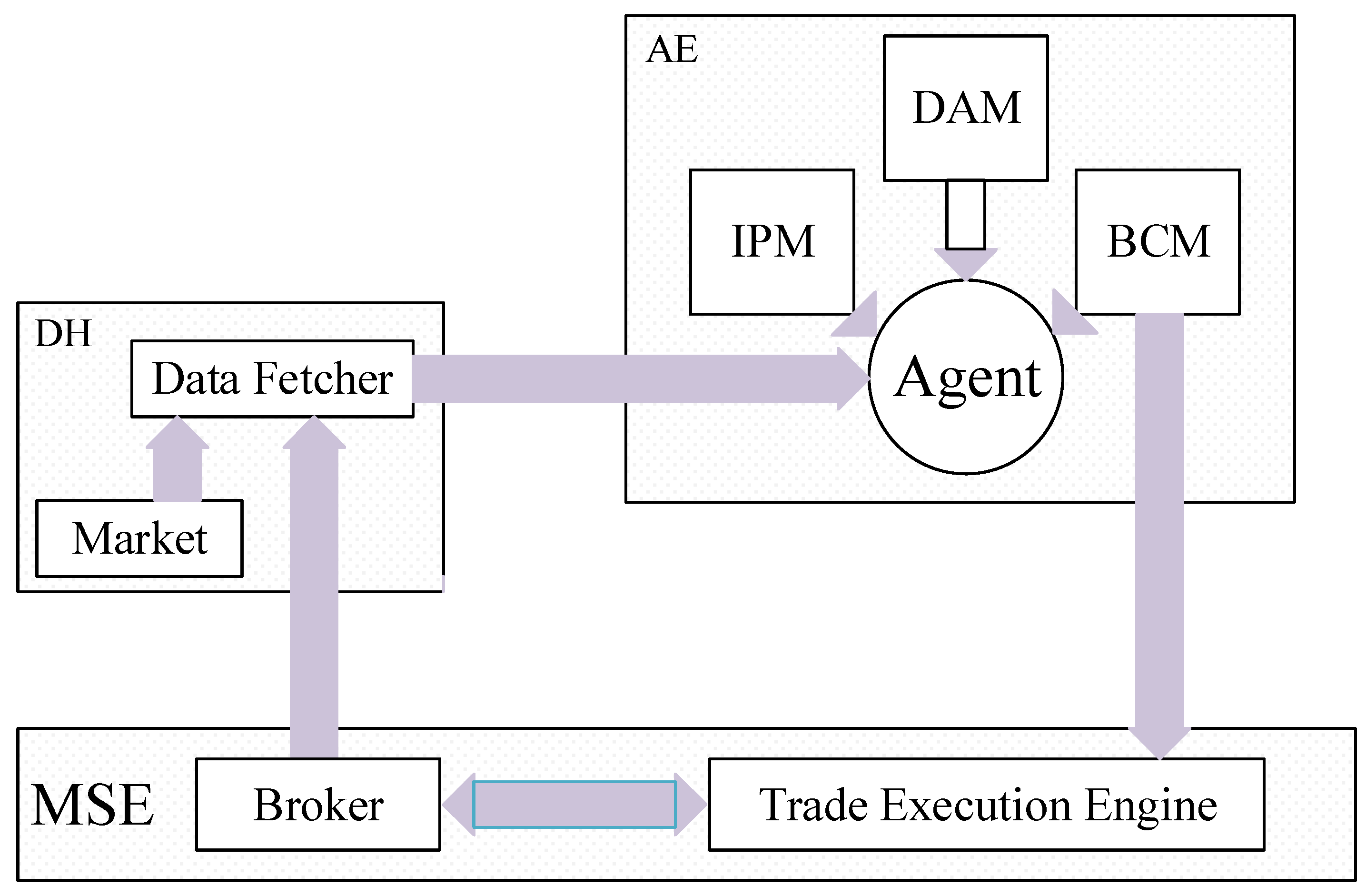
- Proposing a general architecture of DRL in economics.
- Presenting open issues and challenges in current deep reinforcement learning models in economics.
2. Methodology and Taxonomy of the Survey
2.1. Deep Learning Methods
2.2. Stacked Auto-Encoders (SAEs)
2.3. Deep Belief Networks (DBNs)
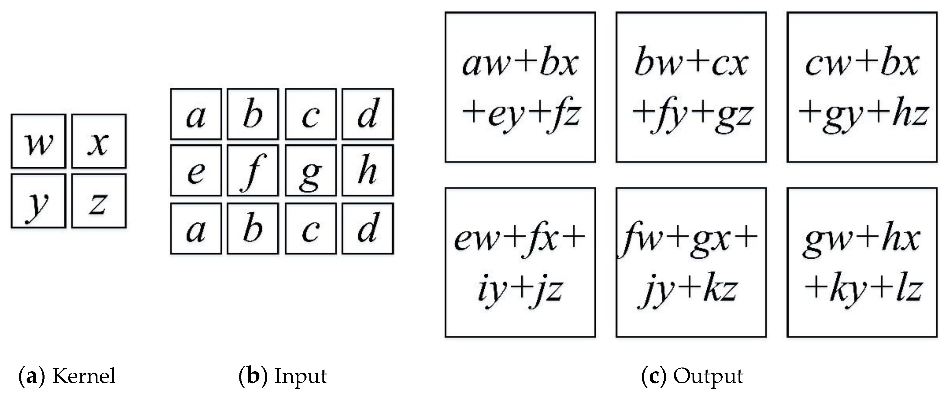
2.4. Convolutional Neural Networks (CNNs)
2.5. Recurrent Neural Networks (RNNs)
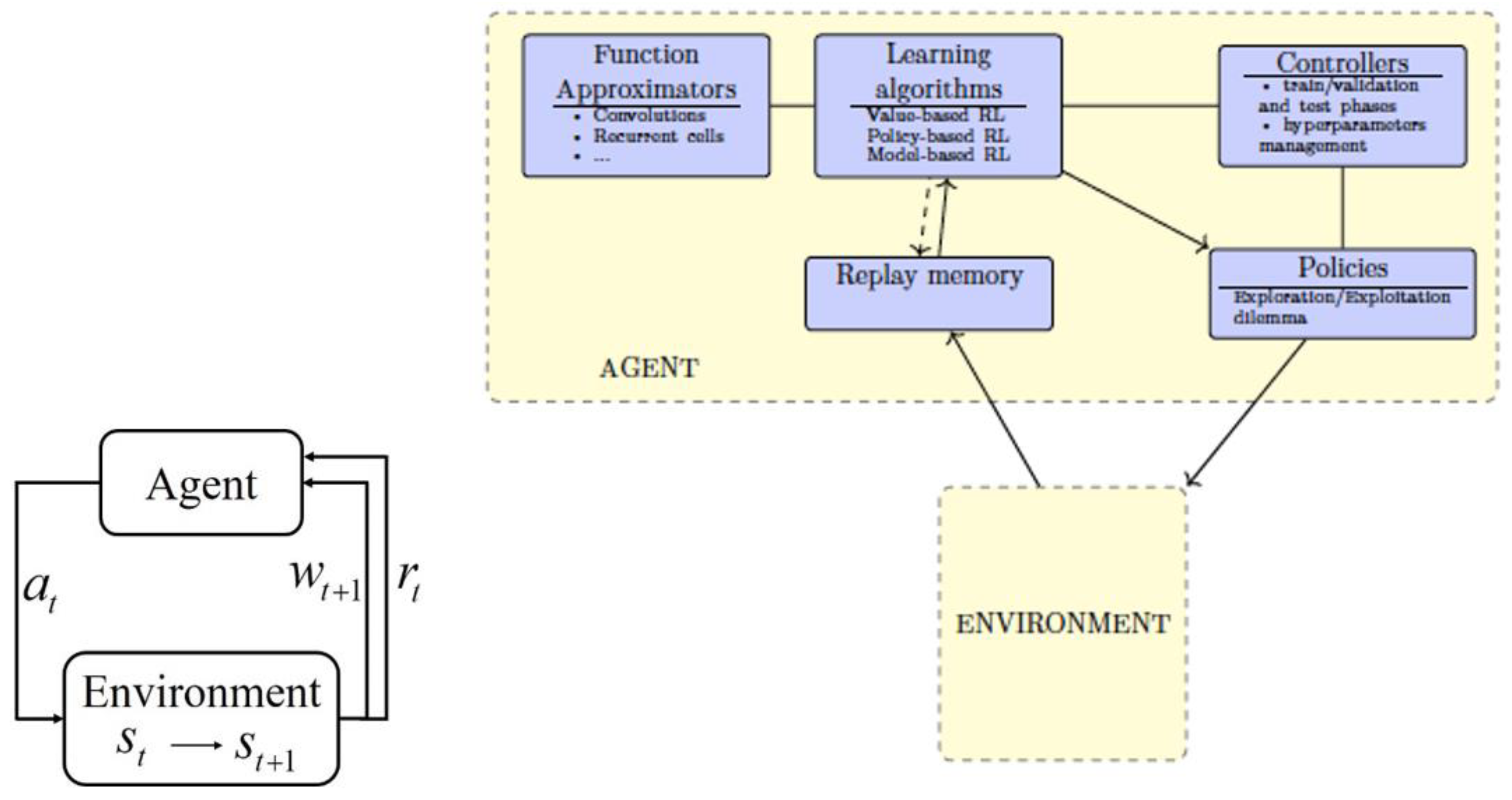
2.6. Deep Reinforcement Learning Methods
2.6.1. Value-Based Methods
2.6.2. Q-Learning
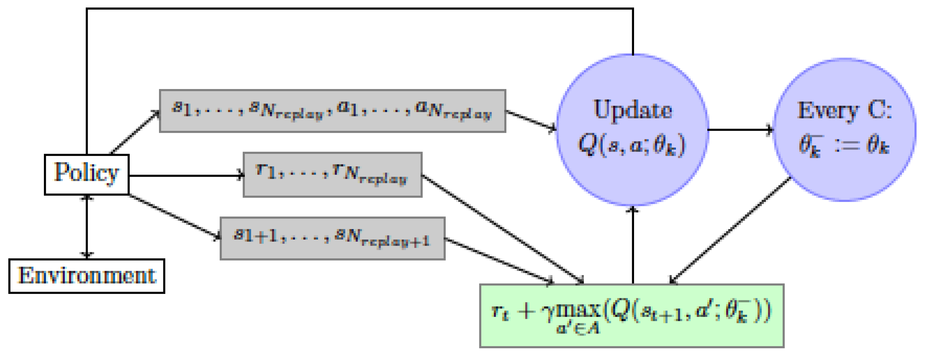
2.6.3. Deep Q-Networks (DQN)
2.6.4. Double DQN
2.6.5. Distributional DQN
2.7. Policy Gradient Methods
2.7.1. Stochastic Policy Gradient (SPG)
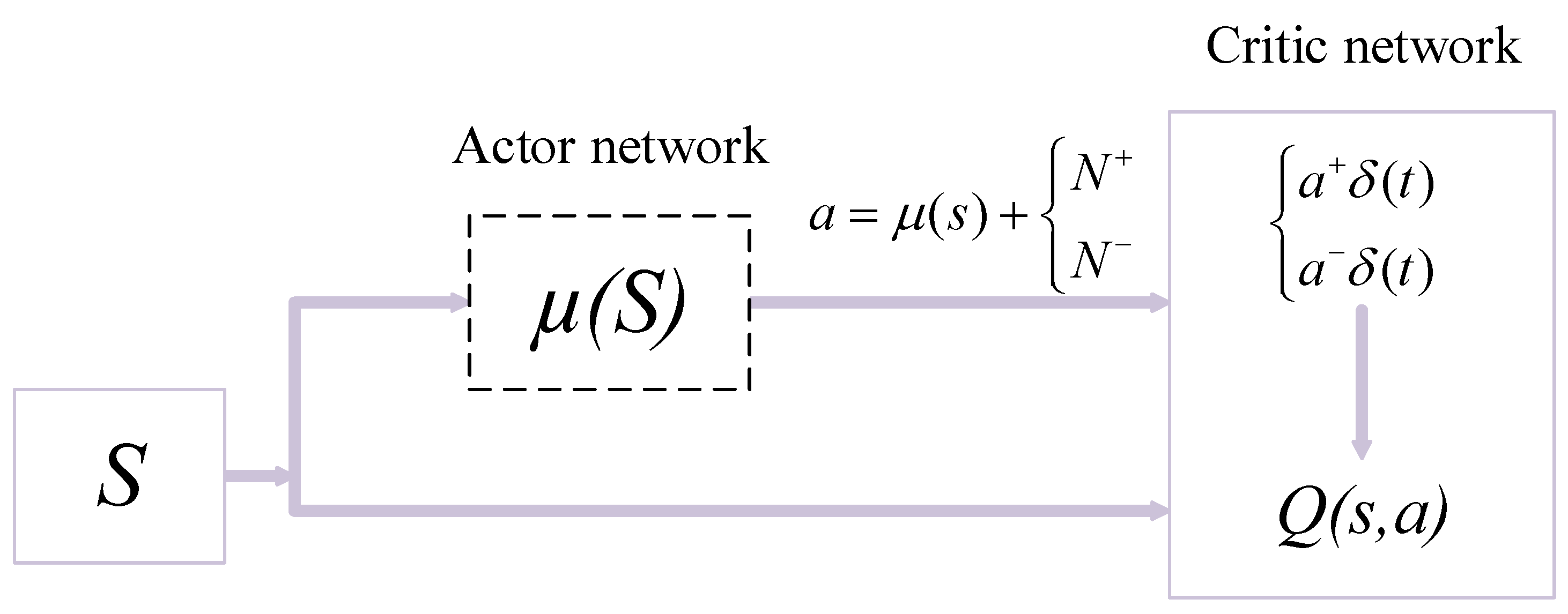
2.7.2. Deterministic Policy Gradient (DPG)
2.7.3. Actor–Critic Methods
2.7.4. Combined Policy Gradient and Q-Learning
2.8. Model-Based Methods
2.8.1. Pure Model-Based Methods
2.8.2. Integrating Model-Free and Model-Based Methods (IMF&MBM)
3. Review Section
3.1. Deep Learning Application in Economics
3.1.1. Deep Learning in Stock Pricing
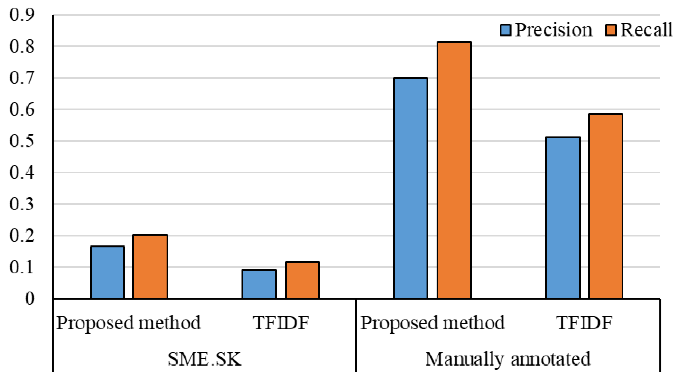
3.1.2. Deep Learning in Insurance
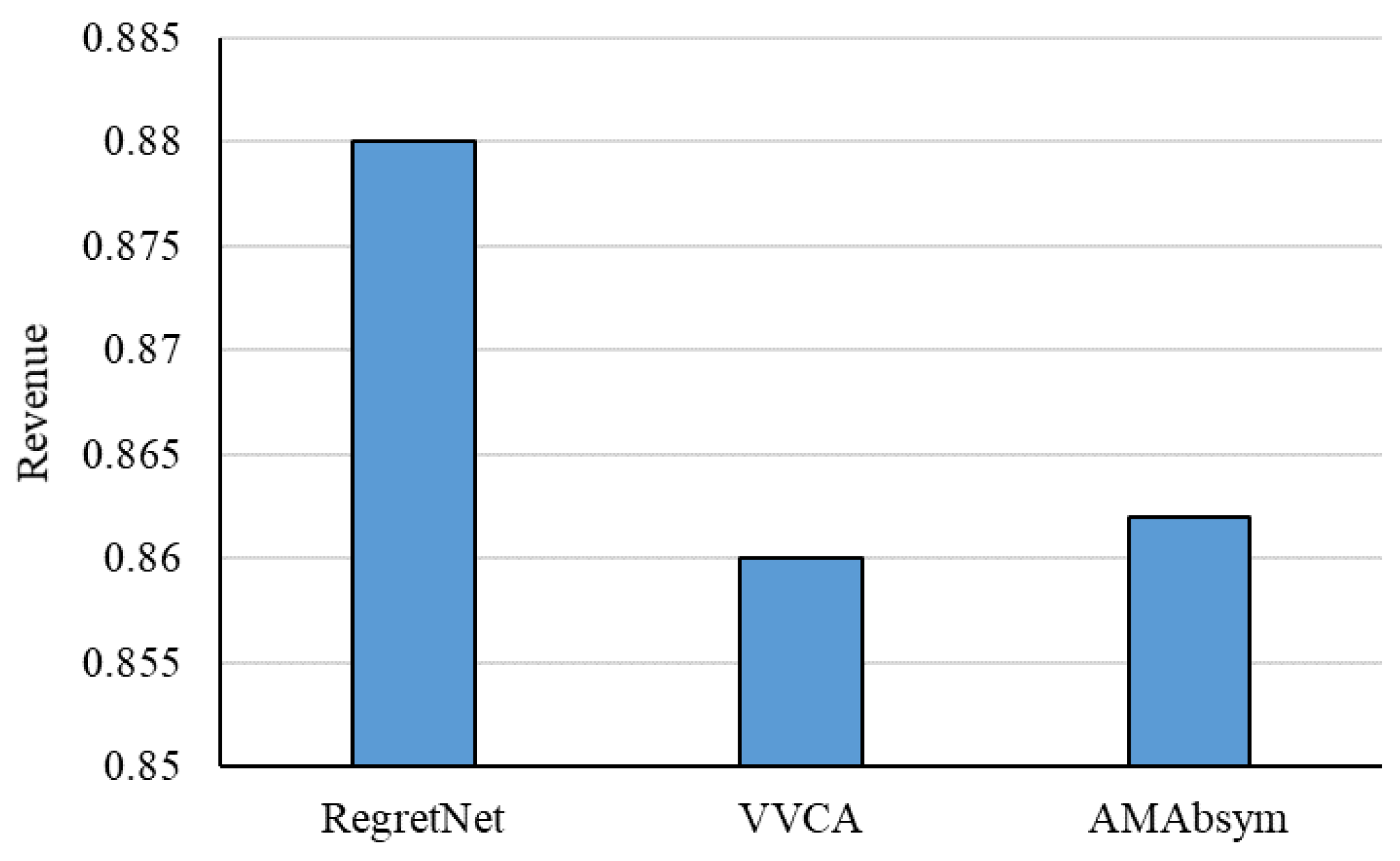
3.1.3. Deep Learning in Auction Mechanisms
3.1.4. Deep Learning in Banking and Online Markets
| Algorithm 1. AE pseudo algorithm | |
| Steps | Processes |
| Step 1:Prepare the input data | Input Matrix X II input dataset Parameter of the matrix//parameter (w,bx,bh) where: w: Weight between layers, bx Encoder’s parameters, bh Decoder’s Parameters |
| Step 2: initial Variables | h←null // vector for the hidden layer X←null // Reconstructed x L←null II vector for Loss Function 1←batch number i←0 |
| Step 3: loop statement | While i < 1 do II Encoder function maps an input X to hidden representation h: h = f (p[i ].w + p[i] bx) /* Decoder function maps hidden representation h back to a Reconstruction X:*/ X = g(p[i ].l/ + p[i] bx) /*For nonlinear reconstruction, the reconstruction loss is generally from cross-entropy :*/ L = −sum(x *log(X) + (1 − x) *log(l − X)) /* For linear reconstruction, the reconstruction loss is generally from the squared error:*/ L = sum(x − X)2 Min θ[i] = p L(x − X) End while Return θ |
| Step 4: output | θ←<null matrix>//objective function /*Training an auto-encoder involves finding parameters = (W,hx,bb) that minimize the reconstruction loss in the given dataset X and the objective function*/ |
3.1.5. Deep Learning in Macroeconomics
3.1.6. Deep Learning in Financial Markets (Service & Risk Management)
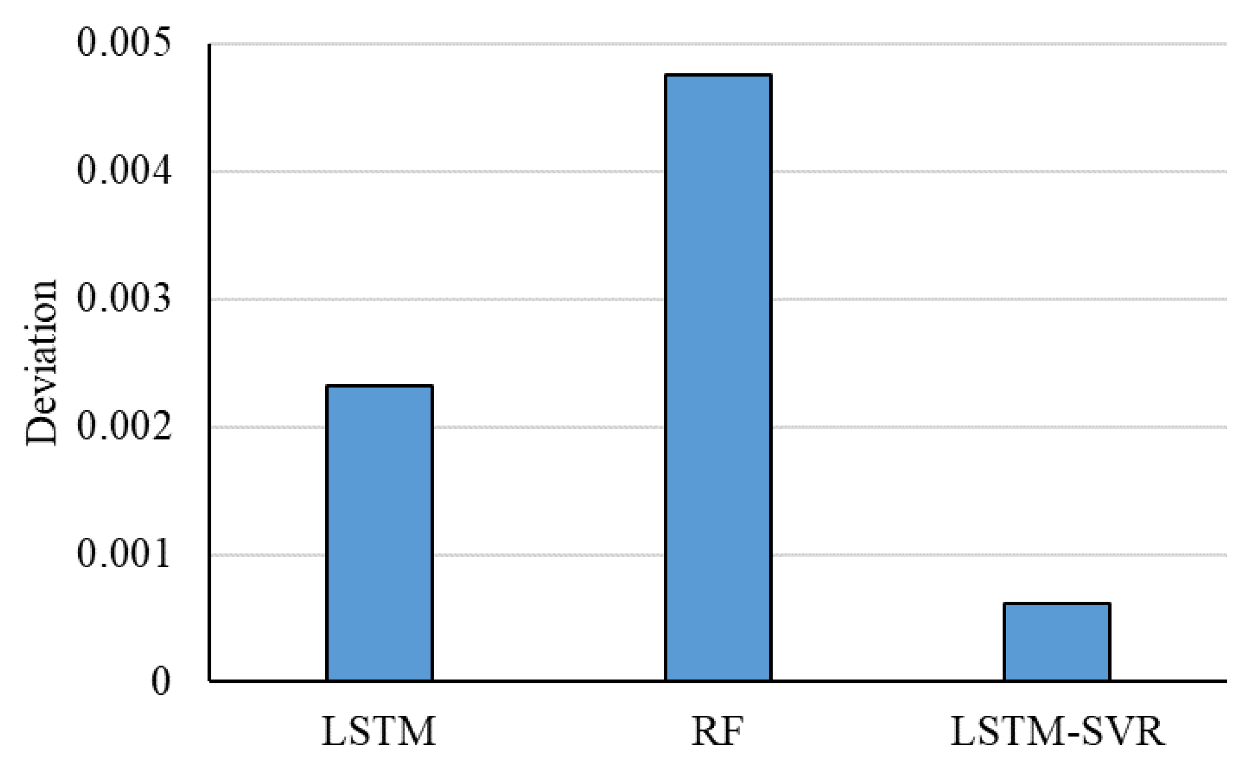
3.1.7. Deep Learning in Investment
3.1.8. Deep Learning in Retail
3.1.9. Deep Learning in Business (Intelligence)
3.2. Deep Reinforcement Learning Application in Economics
3.3. Deep Reinforcement Learning in Stock Trading
3.3.1. Deep Reinforcement Learning in Portfolio Management
3.3.2. Deep Reinforcement Learning in Online Services
| Algorithm 2 [117]: DQN Leaming |
| 1: for epsode = 1 to n do |
| 2: Initialize replay memory D to capacity N |
| 3: Initialize action value functions (Qtrain.Qep. Qtarget) |
| with weights Otrain.Oep.Otarget |
| 4: for t = 1 to m do |
| 5: With probability E select a random action at |
| 6: otherwise select at = arg max 0 Qep(St, a;θep ) |
| 7: Execute action at to auction simulator and observe |
| state St+I and reward rt |
| 8: if budget of St+ 1 < 0, then continue |
| 9: Store transition (s1,at,r1, s1+1 ) in D |
| 10: Sample random rmru batch of transitions |
| (sj,aj,rj, Sj+1 ) from D |
| 11: if j = m then |
| 12: Set Yi = ri |
| 13: else |
| 14: Set Yi = ri + y arg maxa, Qiarget (si+1• a.,θtarget) |
| 15: end if |
| 16: Perform a gradient descent step on the loss function |
| (Yi − Qirain(si.ai;θ1rain)) 2 |
| 17: end for |
| 18: Update θep with θ |
| 19: Every C steps, update θ1arget with θ |
| 20: end for |
4. Discussion
5. Conclusions
Author Contributions
Funding
Acknowledgments
Conflicts of Interest
Abbreviations
| AE | Autoencoder |
| ALT | Augmented Lagrangian Technique |
| ARIMA | Autoregressive Integrated Moving Average |
| BCM | Behavior Cloning Module |
| BI | Business Intelligence |
| CNN | Convolutional Neural Network |
| CNNR | Convolutional Neural Network Regression |
| DAM | Data Augmentation Module |
| DBNs | Deep Belief Networks |
| DDPG | Deterministic Policy Gradient |
| DDQN | Double Deep Q-network |
| DDRL | Deep Deterministic Reinforcement Learning |
| DL | Deep Learning |
| DNN | Deep Neural Network |
| DPG | Deterministic Policy Gradient |
| DQN | Deep Q-network |
| DRL | Deep Reinforcement Learning |
| EIIE | Ensemble of Identical Independent Evaluators |
| ENDE | Encoder-Decoder |
| GANs | Generative Adversarial Nets |
| IPM | Infused Prediction Module |
| LDA | Latent Dirichlet Allocation |
| MARL | Multi-agent Reinforcement Learning |
| MCTS | Monte-Carlo Tree Search |
| MDP | Markov Decision Process |
| MFGs | Mean Field Games |
| ML | Machine Learning |
| MLP | Multilayer Perceptron |
| MLS | Multi Layer Selection |
| NFQCA | Neural Fitted Q Iteration with Continuous Actions |
| NLP | Natural Language Processing |
| OSBL | Online Stochastic Batch Learning |
| PCA | Principal Component Analysis |
| PDE | Partial Differential Equations |
| PG | Policy Gradient |
| PPO | Proximal Policy Optimization |
| PVM | Portfolio-Vector Memory |
| RBM | Restricted Boltzmann Machine |
| RCNN | Recurrent Convolutional Neural Network |
| RL | Reinforcement Learning |
| RNN | Recurrent Neural Network |
| R-NN | Random Neural Network |
| RS | Risk Score |
| RTB | Real-Time Bidding |
| SAE | Stacked Auto-encoder |
| SPF | Survey of Professional Forecasters |
| SPG | Stochastic Policy Gradient |
| SS | Sponsored Search |
| SVR | Support Vector Regression |
| TGRU | Two-Stream Gated Recurrent Unit |
| UCRP | Uniform Constant Rebalanced Portfolios |
References
- Erhan, D.; Bengio, Y.; Courville, A.; Vincent, P. Visualizing higher-layer features of a deep network. Univ. Montr. 2009, 1341, 1. [Google Scholar]
- Olah, C.; Mordvintsev, A.; Schubert, L. Feature visualization. Distill 2017, 2, e7. [Google Scholar] [CrossRef]
- Ding, X.; Zhang, Y.; Liu, T.; Duan, J. Deep learning for event-driven stock prediction. In Proceedings of the Twenty-Fourth International Joint Conference on Artificial Intelligence, Buenos Aires, Argentina, 25–31 July 2015. [Google Scholar]
- Pacelli, V.; Azzollini, M. An artificial neural network approach for credit risk management. J. Intell. Learn. Syst. Appl. 2011, 3, 103–112. [Google Scholar] [CrossRef] [Green Version]
- Srivastava, N.; Hinton, G.; Krizhevsky, A.; Sutskever, I.; Salakhutdinov, R. Dropout: A simple way to prevent neural networks from overfitting. J. Mach. Learn. Res. 2014, 15, 1929–1958. [Google Scholar]
- Mnih, V.; Kavukcuoglu, K.; Silver, D.; Rusu, A.A.; Veness, J.; Bellemare, M.G.; Graves, A.; Riedmiller, M.; Fidjeland, A.K.; Ostrovski, G. Human-level control through deep reinforcement learning. Nature 2015, 518, 529–533. [Google Scholar] [CrossRef] [PubMed]
- Sutton, R.S. Generalization in reinforcement learning: Successful examples using sparse coarse coding. In Proceedings of the Advances in Neural Information Processing Systems 9, Los Angeles, CA, USA, September 1996; pp. 1038–1044. [Google Scholar]
- Arulkumaran, K.; Deisenroth, M.P.; Brundage, M.; Bharath, A.A. Deep reinforcement learning: A brief survey. IEEE Signal Process. Mag. 2017, 34, 26–38. [Google Scholar] [CrossRef] [Green Version]
- Moody, J.; Wu, L.; Liao, Y.; Saffell, M. Performance functions and reinforcement learning for trading systems and portfolios. J. Forecast. 1998, 17, 441–470. [Google Scholar] [CrossRef]
- Dempster, M.A.; Payne, T.W.; Romahi, Y.; Thompson, G.W. Computational learning techniques for intraday FX trading using popular technical indicators. IEEE Trans. Neural Netw. 2001, 12, 744–754. [Google Scholar] [CrossRef]
- Bekiros, S.D. Heterogeneous trading strategies with adaptive fuzzy actor–critic reinforcement learning: A behavioral approach. J. Econ. Dyn. Control 2010, 34, 1153–1170. [Google Scholar] [CrossRef]
- Kearns, M.; Nevmyvaka, Y. Machine learning for market microstructure and high frequency trading. In High Frequency Trading: New Realities for Traders, Markets, and Regulators; Easley, D., de Prado, M.L., O’Hara, M., Eds.; Risk Books: London, UK, 2013. [Google Scholar]
- Britz, D. Introduction to Learning to Trade with Reinforcement Learning. Available online: http://www.wildml.com/2018/02/introduction-to-learning-to-tradewith-reinforcement-learning (accessed on 1 August 2018).
- Guo, Y.; Fu, X.; Shi, Y.; Liu, M. Robust log-optimal strategy with reinforcement learning. arXiv 2018, arXiv:1805.00205. [Google Scholar]
- Jiang, Z.; Xu, D.; Liang, J. A deep reinforcement learning framework for the financial portfolio management problem. arXiv 2017, arXiv:1706.10059. [Google Scholar]
- Nosratabadi, S.; Mosavi, A.; Duan, P.; Ghamisi, P. Data science in economics. arXiv 2020, arXiv:2003.13422. [Google Scholar]
- Chen, Y.; Lin, Z.; Zhao, X.; Wang, G.; Gu, Y. Deep learning-based classification of hyperspectral data. IEEE J. Sel. Top. Appl. Earth Obs. Remote Sens. 2014, 7, 2094–2107. [Google Scholar] [CrossRef]
- Chen, Y.; Zhao, X.; Jia, X. Spectral–spatial classification of hyperspectral data based on deep belief network. IEEE J. Sel. Top. Appl. Earth Obs. Remote Sens. 2015, 8, 2381–2392. [Google Scholar] [CrossRef]
- Krizhevsky, A.; Sutskever, I.; Hinton, G.E. Imagenet classification with deep convolutional neural networks. In Proceedings of the Advances in Neural Information Processing Systems 25, Los Angeles, CA, USA, 1 June 2012; pp. 1097–1105. [Google Scholar]
- Bengio, Y.; Simard, P.; Frasconi, P. Learning long-term dependencies with gradient descent is difficult. IEEE Trans. Neural Netw. 1994, 5, 157–166. [Google Scholar] [CrossRef]
- Williams, R.J.; Zipser, D. A learning algorithm for continually running fully recurrent neural networks. Neural Comput. 1989, 1, 270–280. [Google Scholar] [CrossRef]
- Schmidhuber, J.; Hochreiter, S. Long short-term memory. Neural Comput. 1997, 9, 1735–1780. [Google Scholar]
- Chung, J.; Gulcehre, C.; Cho, K.; Bengio, Y. Empirical evaluation of gated recurrent neural networks on sequence modeling. arXiv 2014, arXiv:1412.3555. [Google Scholar]
- Wu, J. Introduction to Convolutional Neural Networks; National Key Lab for Novel Software Technology, Nanjing University: Nanjing, China, 2017; Volume 5, p. 23. [Google Scholar]
- François-Lavet, V.; Henderson, P.; Islam, R.; Bellemare, M.G.; Pineau, J. An introduction to deep reinforcement learning. Found. Trends® Mach. Learn. 2018, 11, 219–354. [Google Scholar] [CrossRef] [Green Version]
- Watkins, C.J.; Dayan, P. Q-learning. Mach. Learn. 1992, 8, 279–292. [Google Scholar] [CrossRef]
- Bellman, R.E.; Dreyfus, S. Applied Dynamic Programming; Princeton University Press: Princeton, NJ, USA, 1962. [Google Scholar]
- Lin, L.-J. Self-improving reactive agents based on reinforcement learning, planning and teaching. Mach. Learn. 1992, 8, 293–321. [Google Scholar] [CrossRef]
- Tieleman, T.; Hinton, G. Lecture 6.5-rmsprop: Divide the gradient by a running average of its recent magnitude. COURSERA Neural Netw. Mach. Learn. 2012, 4, 26–31. [Google Scholar]
- Hasselt, H.V. Double Q-learning. In Proceedings of the Advances in Neural Information Processing Systems 23, San Diego, CA, USA, July 2010; pp. 2613–2621. [Google Scholar]
- Bellemare, M.G.; Dabney, W.; Munos, R. A distributional perspective on reinforcement learning. In Proceedings of the 34th International Conference on Machine Learning, Sydney, Australia, 6–11 August 2017; Volume 70, pp. 449–458. [Google Scholar]
- Dabney, W.; Rowland, M.; Bellemare, M.G.; Munos, R. Distributional reinforcement learning with quantile regression. In Proceedings of the Thirty-Second AAAI Conference on Artificial Intelligence, New Orleans, LA, USA, 2–7 February 2018. [Google Scholar]
- Rowland, M.; Bellemare, M.G.; Dabney, W.; Munos, R.; Teh, Y.W. An analysis of categorical distributional reinforcement learning. arXiv 2018, arXiv:1802.08163. [Google Scholar]
- Morimura, T.; Sugiyama, M.; Kashima, H.; Hachiya, H.; Tanaka, T. Nonparametric return distribution approximation for reinforcement learning. In Proceedings of the 27th International Conference on Machine Learning (ICML-10), Haifa, Israel, 21–24 June 2010; pp. 799–806. [Google Scholar]
- Jaderberg, M.; Mnih, V.; Czarnecki, W.M.; Schaul, T.; Leibo, J.Z.; Silver, D.; Kavukcuoglu, K. Reinforcement learning with unsupervised auxiliary tasks. arXiv 2016, arXiv:1611.05397. [Google Scholar]
- Mnih, V.; Badia, A.P.; Mirza, M.; Graves, A.; Lillicrap, T.; Harley, T.; Silver, D.; Kavukcuoglu, K. Asynchronous methods for deep reinforcement learning. In Proceedings of the 12th International Conference, MLDM 2016, New York, NY, USA, 18–20 July 2016; Springer: Berlin/Heidelberg, Germany, 2016; Volume 9729. [Google Scholar]
- Salimans, T.; Ho, J.; Chen, X.; Sidor, S.; Sutskever, I. Evolution strategies as a scalable alternative to reinforcement learning. arXiv 2017, arXiv:1703.03864. [Google Scholar]
- Williams, R.J. Simple statistical gradient-following algorithms for connectionist reinforcement learning. Mach. Learn. 1992, 8, 229–256. [Google Scholar] [CrossRef] [Green Version]
- Silver, D.; Lever, G.; Heess, N.; Degris, T.; Wierstra, D.; Riedmiller, M. Deterministic policy gradient algorithms. In Proceedings of the 31st International Conference on International Conference on Machine Learning, Beijing, China, 21–26 June 2014. [Google Scholar]
- Hafner, R.; Riedmiller, M. Reinforcement learning in feedback control. Mach. Learn. 2011, 84, 137–169. [Google Scholar] [CrossRef] [Green Version]
- Lillicrap, T.P.; Hunt, J.J.; Pritzel, A.; Heess, N.; Erez, T.; Tassa, Y.; Silver, D.; Wierstra, D. Continuous control with deep reinforcement learning. arXiv 2015, arXiv:1509.02971. [Google Scholar]
- Konda, V.R.; Tsitsiklis, J.N. Actor-critic algorithms. In Proceedings of the Advances in Neural Information Processing Systems 12, Chicago, IL, USA, 20 June 2000; pp. 1008–1014. [Google Scholar]
- Wang, Z.; Bapst, V.; Heess, N.; Mnih, V.; Munos, R.; Kavukcuoglu, K.; de Freitas, N. Sample efficient actor-critic with experience replay. arXiv 2016, arXiv:1611.01224. [Google Scholar]
- Gruslys, A.; Azar, M.G.; Bellemare, M.G.; Munos, R. The reactor: A sample-efficient actor-critic architecture. arXiv 2017, arXiv:1704.04651. [Google Scholar]
- O’Donoghue, B.; Munos, R.; Kavukcuoglu, K.; Mnih, V. Combining policy gradient and Q-learning. arXiv 2016, arXiv:1611.01626. [Google Scholar]
- Fox, R.; Pakman, A.; Tishby, N. Taming the noise in reinforcement learning via soft updates. arXiv 2015, arXiv:1512.08562. [Google Scholar]
- Haarnoja, T.; Tang, H.; Abbeel, P.; Levine, S. Reinforcement learning with deep energy-based policies. In Proceedings of the 34th International Conference on Machine Learning, Sydney, Australia, 6–11 August 2017; Volume 70, pp. 1352–1361. [Google Scholar]
- Schulman, J.; Chen, X.; Abbeel, P. Equivalence between policy gradients and soft q-learning. arXiv 2017, arXiv:1704.06440. [Google Scholar]
- Oh, J.; Guo, X.; Lee, H.; Lewis, R.L.; Singh, S. Action-conditional video prediction using deep networks in atari games. In Proceedings of the Advances in Neural Information Processing Systems 28: 29th Annual Conference on Neural Information Processing Systems, Seattle, WA, USA, May 2015; pp. 2863–2871. [Google Scholar]
- Mathieu, M.; Couprie, C.; LeCun, Y. Deep multi-scale video prediction beyond mean square error. arXiv 2015, arXiv:1511.05440. [Google Scholar]
- Finn, C.; Goodfellow, I.; Levine, S. Unsupervised learning for physical interaction through video prediction. In Proceedings of the Advances in Neural Information Processing Systems Advances in Neural Information, Processing Systems 29, Barcelona, Spain, 5–10 December 2016; pp. 64–72. [Google Scholar]
- Pascanu, R.; Li, Y.; Vinyals, O.; Heess, N.; Buesing, L.; Racanière, S.; Reichert, D.; Weber, T.; Wierstra, D.; Battaglia, P. Learning model-based planning from scratch. arXiv 2017, arXiv:1707.06170. [Google Scholar]
- Deisenroth, M.; Rasmussen, C.E. PILCO: A model-based and data-efficient approach to policy search. In Proceedings of the 28th International Conference on Machine Learning (ICML-11), Bellevue, WA, USA, 28 June–2 July 2011; pp. 465–472. [Google Scholar]
- Wahlström, N.; Schön, T.B.; Deisenroth, M.P. From pixels to torques: Policy learning with deep dynamical models. arXiv 2015, arXiv:1502.02251. [Google Scholar]
- Levine, S.; Koltun, V. Guided policy search. In Proceedings of the International Conference on Machine Learning, Oslo, Norway, February 2013; pp. 1–9. [Google Scholar]
- Gu, S.; Lillicrap, T.; Sutskever, I.; Levine, S. Continuous deep q-learning with model-based acceleration. In Proceedings of the International Conference on Machine Learning(ICML 2013), Atlanta, GA, USA, June 2013; pp. 2829–2838. [Google Scholar]
- Nagabandi, A.; Kahn, G.; Fearing, R.S.; Levine, S. Neural network dynamics for model-based deep reinforcement learning with model-free fine-tuning. In Proceedings of the 2018 IEEE International Conference on Robotics and Automation (ICRA), Brisbane, Australia, 21–26 May 2018; pp. 7559–7566. [Google Scholar]
- Silver, D.; Huang, A.; Maddison, C.J.; Guez, A.; Sifre, L.; Van Den Driessche, G.; Schrittwieser, J.; Antonoglou, I.; Panneershelvam, V.; Lanctot, M. Mastering the game of Go with deep neural networks and tree search. Nature 2016, 529, 484–489. [Google Scholar] [CrossRef]
- Heess, N.; Wayne, G.; Silver, D.; Lillicrap, T.; Erez, T.; Tassa, Y. Learning continuous control policies by stochastic value gradients. In Proceedings of the Advances in Neural Information Processing Systems; Annual Conference on Neural Information Processing Systems, Montreal, QC, Canada, December 2015; pp. 2944–2952. [Google Scholar]
- Kansky, K.; Silver, T.; Mély, D.A.; Eldawy, M.; Lázaro-Gredilla, M.; Lou, X.; Dorfman, N.; Sidor, S.; Phoenix, S.; George, D. Schema networks: Zero-shot transfer with a generative causal model of intuitive physics. In Proceedings of the 34th International Conference on Machine Learning, Sydney, Australia, 6–11 August 2017; Volume 70, pp. 1809–1818. [Google Scholar]
- Patel, J.; Shah, S.; Thakkar, P.; Kotecha, K. Predicting stock and stock price index movement using trend deterministic data preparation and machine learning techniques. Expert Syst. Appl. 2015, 42, 259–268. [Google Scholar] [CrossRef]
- Lien Minh, D.; Sadeghi-Niaraki, A.; Huy, H.D.; Min, K.; Moon, H. Deep learning approach for short-term stock trends prediction based on two-stream gated recurrent unit network. IEEE Access 2018, 6, 55392–55404. [Google Scholar] [CrossRef]
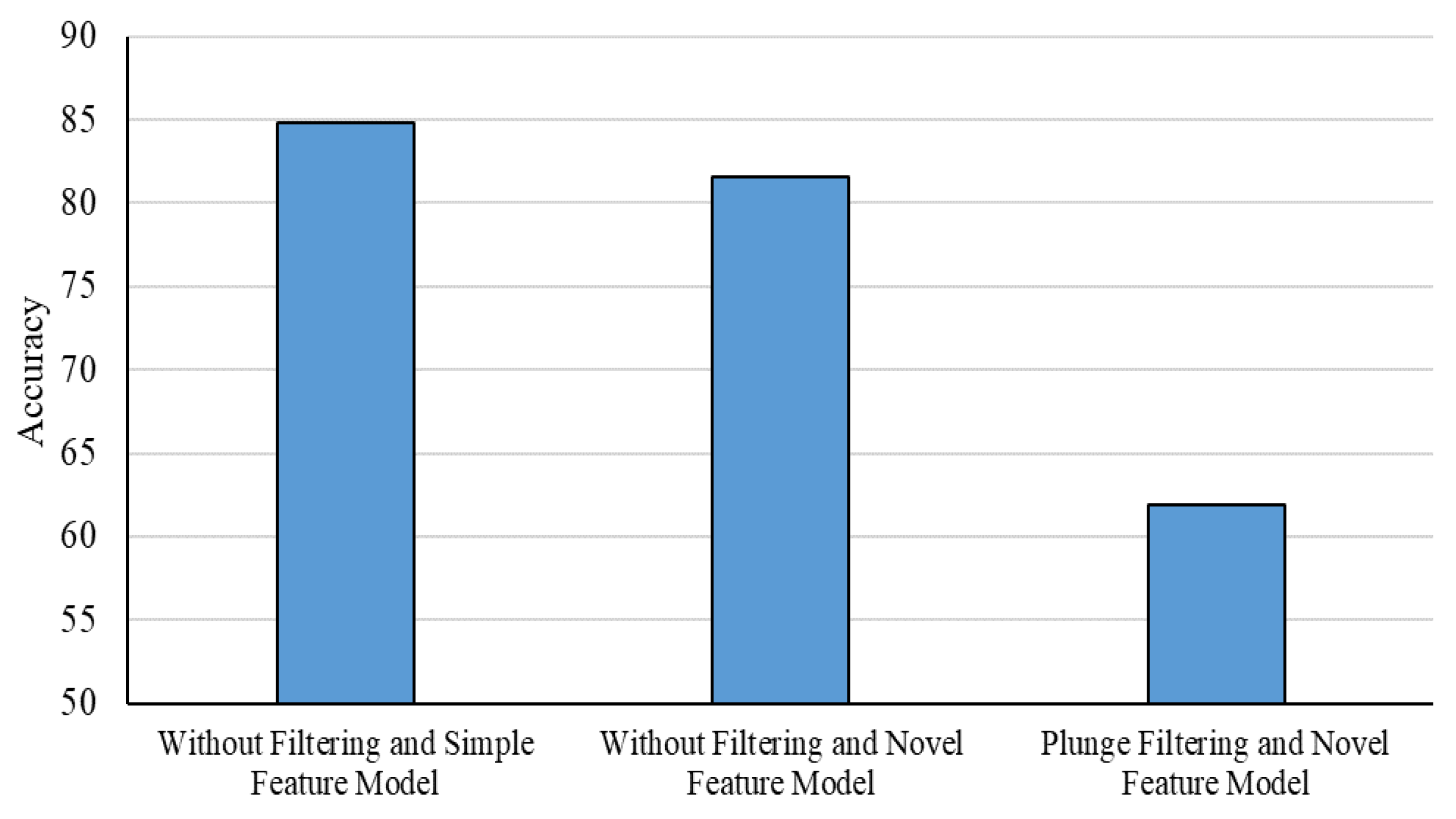
- Song, Y.; Lee, J.W.; Lee, J. A study on novel filtering and relationship between input-features and target-vectors in a deep learning model for stock price prediction. Appl. Intell. 2019, 49, 897–911. [Google Scholar] [CrossRef]
- Go, Y.H.; Hong, J.K. Prediction of stock value using pattern matching algorithm based on deep learning. Int. J. Recent Technol. Eng. 2019, 8, 31–35. [Google Scholar] [CrossRef]
- Das, S.; Mishra, S. Advanced deep learning framework for stock value prediction. Int. J. Innov. Technol. Explor. Eng. 2019, 8, 2358–2367. [Google Scholar] [CrossRef]
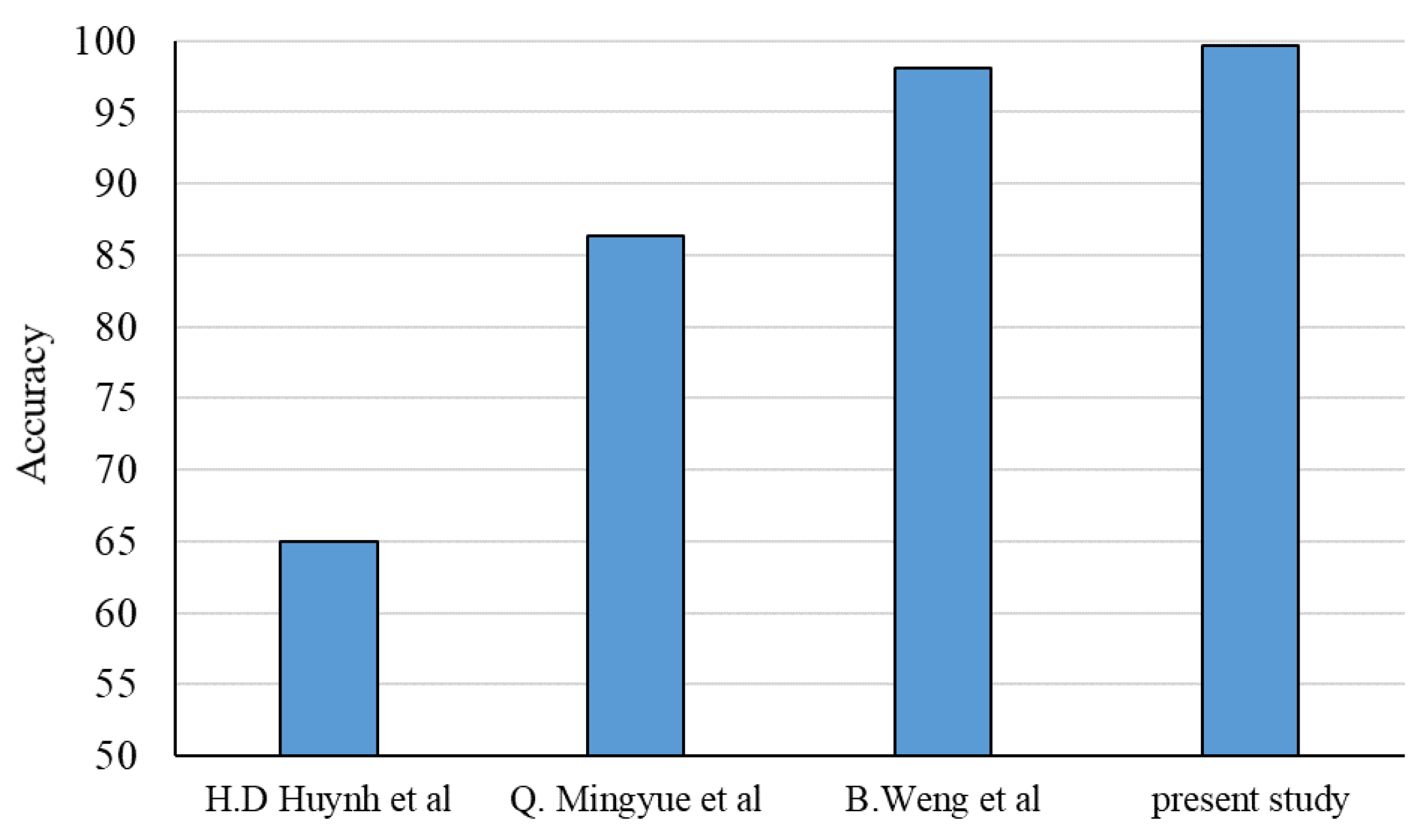
- Huynh, H.D.; Dang, L.M.; Duong, D. A new model for stock price movements prediction using deep neural network. In Proceedings of the Eighth International Symposium on Information and Communication Technology, Ann Arbor, MI, USA, June 2016; pp. 57–62. [Google Scholar]
- Mingyue, Q.; Cheng, L.; Yu, S. Application of the artifical neural network in predicting the direction of stock market index. In Proceedings of the 2016 10th International Conference on Complex, Intelligent, and Software Intensive Systems (CISIS), Fukuoka, Japan, 6–8 July 2016; pp. 219–223. [Google Scholar]
- Weng, B.; Martinez, W.; Tsai, Y.T.; Li, C.; Lu, L.; Barth, J.R.; Megahed, F.M. Macroeconomic indicators alone can predict the monthly closing price of major US indices: Insights from artificial intelligence, time-series analysis and hybrid models. Appl. Soft Comput. 2017, 71, 685–697. [Google Scholar] [CrossRef]
- Bodaghi, A.; Teimourpour, B. The detection of professional fraud in automobile insurance using social network analysis. arXiv 2018, arXiv:1805.09741. [Google Scholar]
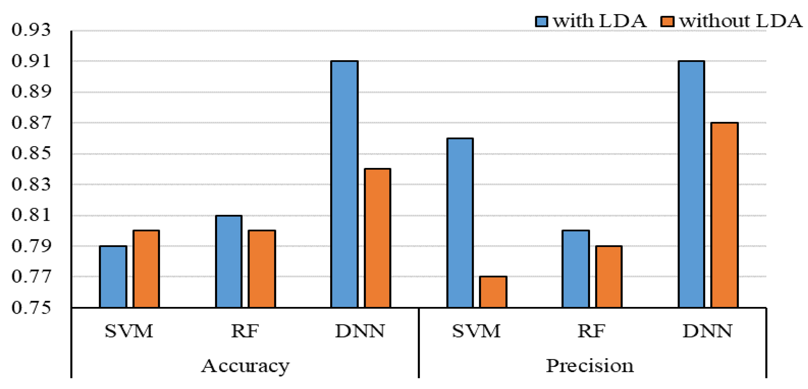
- Wang, Y.; Xu, W. Leveraging deep learning with LDA-based text analytics to detect automobile insurance fraud. Decis. Support Syst. 2018, 105, 87–95. [Google Scholar] [CrossRef]
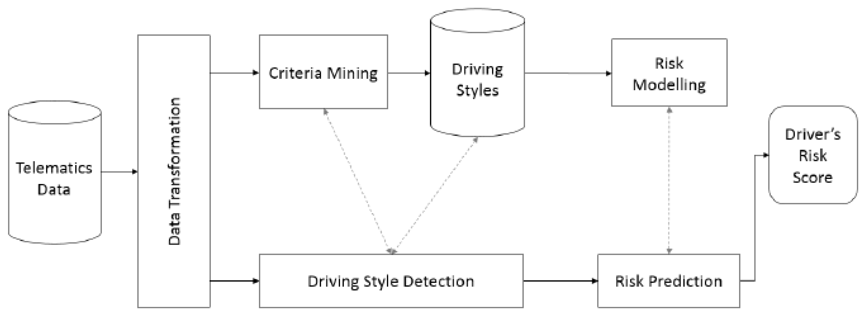
- Siaminamini, M.; Naderpour, M.; Lu, J. Generating a risk profile for car insurance policyholders: A deep learning conceptual model. In Proceedings of the Australasian Conference on Information Systems, Geelong, Australia, 3–5 December 2012. [Google Scholar]
- Myerson, R.B. Optimal auction design. Math. Oper. Res. 1981, 6, 58–73. [Google Scholar] [CrossRef]
- Manelli, A.M.; Vincent, D.R. Bundling as an optimal selling mechanism for a multiple-good monopolist. J. Econ. Theory 2006, 127, 1–35. [Google Scholar] [CrossRef]
- Pavlov, G. Optimal mechanism for selling two goods. BE J. Theor. Econ. 2011, 11, 122–144. [Google Scholar] [CrossRef] [Green Version]
- Cai, Y.; Daskalakis, C.; Weinberg, S.M. An algorithmic characterization of multi-dimensional mechanisms. In Proceedings of the Forty-Fourth Annual ACM Symposium on Theory of Computing; Association for Computing Machinery, New York, NY, USA, 19–22 May 2012; pp. 459–478. [Google Scholar]
- Dutting, P.; Zheng, F.; Narasimhan, H.; Parkes, D. Optimal economic design through deep learning. In Proceedings of the Conference on Neural Information Processing Systems (NIPS), Berlin, Germany, 4–9 December 2017. [Google Scholar]
- Feng, Z.; Narasimhan, H.; Parkes, D.C. Deep learning for revenue-optimal auctions with budgets. In Proceedings of the 17th International Conference on Autonomous Agents and Multiagent Systems, Stockholm, Sweden, 10–15 July 2018; pp. 354–362. [Google Scholar]
- Sakurai, Y.; Oyama, S.; Guo, M.; Yokoo, M. Deep false-name-proof auction mechanisms. In Proceedings of the International Conference on Principles and Practice of Multi-Agent Systems, Kolkata, India, 12–15 November 2010; pp. 594–601. [Google Scholar]
- Luong, N.C.; Xiong, Z.; Wang, P.; Niyato, D. Optimal auction for edge computing resource management in mobile blockchain networks: A deep learning approach. In Proceedings of the 2018 IEEE International Conference on Communications (ICC), Kansas City, MO, USA, 20–24 May 2018; pp. 1–6. [Google Scholar]
- Dütting, P.; Feng, Z.; Narasimhan, H.; Parkes, D.C.; Ravindranath, S.S. Optimal auctions through deep learning. arXiv 2017, arXiv:1706.03459. [Google Scholar]
- Al-Shabi, M. Credit card fraud detection using autoencoder model in unbalanced datasets. J. Adv. Math. Comput. Sci. 2019, 33, 1–16. [Google Scholar] [CrossRef] [Green Version]
- Roy, A.; Sun, J.; Mahoney, R.; Alonzi, L.; Adams, S.; Beling, P. Deep learning detecting fraud in credit card transactions. In Proceedings of the 2018 Systems and Information Engineering Design Symposium (SIEDS), Charlottesville, VA, USA, 27 April 2018; IEEE: Trondheim, Norway, 2018; pp. 129–134. [Google Scholar]
- Han, J.; Barman, U.; Hayes, J.; Du, J.; Burgin, E.; Wan, D. Nextgen aml: Distributed deep learning based language technologies to augment anti money laundering investigation. In Proceedings of the ACL 2018, System Demonstrations, Melbourne, Australia, 15–20 July 2018. [Google Scholar]
- Pumsirirat, A.; Yan, L. Credit card fraud detection using deep learning based on auto-encoder and restricted boltzmann machine. Int. J. Adv. Comput. Sci. Appl. 2018, 9, 18–25. [Google Scholar] [CrossRef]
- Estrella, A.; Hardouvelis, G.A. The term structure as a predictor of real economic activity. J. Financ. 1991, 46, 555–576. [Google Scholar] [CrossRef]
- Smalter Hall, A.; Cook, T.R. Macroeconomic indicator forecasting with deep neural networks. In Federal Reserve Bank of Kansas City Working Paper; Federal Reserve Bank of Kansas City: Kansas City, MO, USA, 2017; Volume 7, pp. 83–120. [Google Scholar] [CrossRef] [Green Version]
- Haider, A.; Hanif, M.N. Inflation forecasting in Pakistan using artificial neural networks. Pak. Econ. Soc. Rev. 2009, 47, 123–138. [Google Scholar]
- Chakravorty, G.; Awasthi, A. Deep learning for global tactical asset allocation. SSRN Electron. J. 2018, 3242432. [Google Scholar] [CrossRef]
- Addo, P.; Guegan, D.; Hassani, B. Credit risk analysis using machine and deep learning models. Risks 2018, 6, 38. [Google Scholar] [CrossRef] [Green Version]
- Ha, V.-S.; Nguyen, H.-N. Credit scoring with a feature selection approach based deep learning. In Proceedings of the MATEC Web of Conferences, Beijing, China, 25–27 May 2018; p. 05004. [Google Scholar]
- Heaton, J.; Polson, N.; Witte, J.H. Deep learning for finance: Deep portfolios. Appl. Stoch. Models Bus. Ind. 2017, 33, 3–12. [Google Scholar] [CrossRef]
- Sirignano, J.; Sadhwani, A.; Giesecke, K. Deep learning for mortgage risk. arXiv 2016, arXiv:1607.02470. [Google Scholar] [CrossRef] [Green Version]
- Aggarwal, S.; Aggarwal, S. Deep investment in financial markets using deep learning models. Int. J. Comput. Appl. 2017, 162, 40–43. [Google Scholar] [CrossRef]
- Culkin, R.; Das, S.R. Machine learning in finance: The case of deep learning for option pricing. J. Invest. Manag. 2017, 15, 92–100. [Google Scholar]
- Fang, Y.; Chen, J.; Xue, Z. Research on quantitative investment strategies based on deep learning. Algorithms 2019, 12, 35. [Google Scholar] [CrossRef] [Green Version]
- Serrano, W. The random neural network with a genetic algorithm and deep learning clusters in fintech: Smart investment. In Proceedings of the IFIP International Conference on Artificial Intelligence Applications and Innovations, Hersonissos, Crete, Greece, 24–26 May 2019; pp. 297–310. [Google Scholar]
- Hutchinson, J.M.; Lo, A.W.; Poggio, T. A nonparametric approach to pricing and hedging derivative securities via learning networks. J. Financ. 1994, 49, 851–889. [Google Scholar] [CrossRef]
- Cruz, E.; Orts-Escolano, S.; Gomez-Donoso, F.; Rizo, C.; Rangel, J.C.; Mora, H.; Cazorla, M. An augmented reality application for improving shopping experience in large retail stores. Virtual Real. 2019, 23, 281–291. [Google Scholar] [CrossRef] [Green Version]
- Loureiro, A.L.; Miguéis, V.L.; da Silva, L.F. Exploring the use of deep neural networks for sales forecasting in fashion retail. Decis. Support Syst. 2018, 114, 81–93. [Google Scholar] [CrossRef]
- Nogueira, V.; Oliveira, H.; Silva, J.A.; Vieira, T.; Oliveira, K. RetailNet: A deep learning approach for people counting and hot spots detection in retail stores. In Proceedings of the 2019 32nd SIBGRAPI Conference on Graphics, Patterns and Images (SIBGRAPI), Rio de Janeiro, Brazil, 28–31 October 2019; pp. 155–162. [Google Scholar]
- Ribeiro, F.D.S.; Caliva, F.; Swainson, M.; Gudmundsson, K.; Leontidis, G.; Kollias, S. An adaptable deep learning system for optical character verification in retail food packaging. In Proceedings of the 2018 IEEE Conference on Evolving and Adaptive Intelligent Systems (EAIS), Rhodes, Greece, 25–27 May 2018; pp. 1–8. [Google Scholar]
- Fombellida, J.; Martín-Rubio, I.; Torres-Alegre, S.; Andina, D. Tackling business intelligence with bioinspired deep learning. Neural Comput. Appl. 2018, 1–8. [Google Scholar] [CrossRef] [Green Version]
- Singh, V.; Verma, N.K. Deep learning architecture for high-level feature generation using stacked auto encoder for business intelligence. In Complex Systems: Solutions and Challenges in Economics, Management and Engineering; Springer: Berlin/Heidelberg, Germany, 2018; pp. 269–283. [Google Scholar]
- Nolle, T.; Seeliger, A.; Mühlhäuser, M. BINet: Multivariate business process anomaly detection using deep learning. In Proceedings of the International Conference on Business Process Management, Sydney, Australia, 9–14 September 2018; pp. 271–287. [Google Scholar]
- Evermann, J.; Rehse, J.-R.; Fettke, P. Predicting process behaviour using deep learning. Decis. Support Syst. 2017, 100, 129–140. [Google Scholar] [CrossRef] [Green Version]
- West, D. Neural network credit scoring models. Comput. Oper. Res. 2000, 27, 1131–1152. [Google Scholar] [CrossRef]
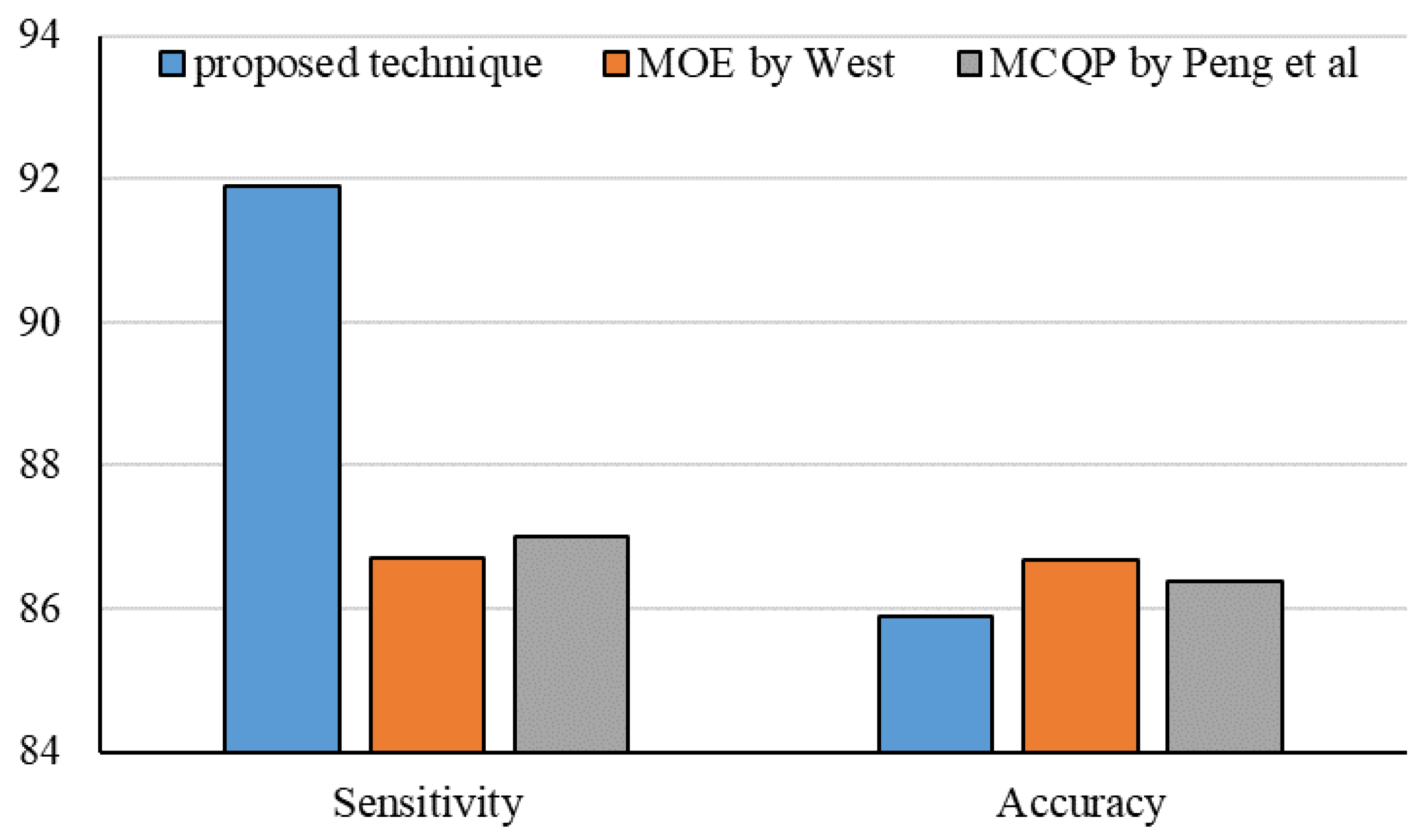
- Peng, Y.; Kou, G.; Shi, Y.; Chen, Z. A multi-criteria convex quadratic programming model for credit data analysis. Decis. Support Syst. 2008, 44, 1016–1030. [Google Scholar] [CrossRef]
- Kim, Y.; Ahn, W.; Oh, K.J.; Enke, D. An intelligent hybrid trading system for discovering trading rules for the futures market using rough sets and genetic algorithms. Appl. Soft Comput. 2017, 55, 127–140. [Google Scholar] [CrossRef]
- Xiong, Z.; Liu, X.-Y.; Zhong, S.; Yang, H.; Walid, A. Practical deep reinforcement learning approach for stock trading. arXiv 2018, arXiv:1811.07522. [Google Scholar]
- Li, X.; Li, Y.; Zhan, Y.; Liu, X.-Y. Optimistic bull or pessimistic bear: Adaptive deep reinforcement learning for stock portfolio allocation. arXiv 2019, arXiv:1907.01503. [Google Scholar]
- Li, Y.; Ni, P.; Chang, V. An empirical research on the investment strategy of stock market based on deep reinforcement learning model. Comput. Sci. Econ. 2019. [Google Scholar] [CrossRef]
- Azhikodan, A.R.; Bhat, A.G.; Jadhav, M.V. Stock Trading Bot Using Deep Reinforcement Learning. In Innovations in Computer Science and Engineering; Springer: Berlin/Heidelberg, Germany, 2019; pp. 41–49. [Google Scholar]
- Liang, Z.; Chen, H.; Zhu, J.; Jiang, K.; Li, Y. Adversarial deep reinforcement learning in portfolio management. arXiv 2018, arXiv:1808.09940. [Google Scholar]
- Jiang, Z.; Liang, J. Cryptocurrency portfolio management with deep reinforcement learning. In Proceedings of the 2017 Intelligent Systems Conference (IntelliSys), London, UK, 7–8 September 2017; pp. 905–913. [Google Scholar]
- Yu, P.; Lee, J.S.; Kulyatin, I.; Shi, Z.; Dasgupta, S. Model-based Deep Reinforcement Learning for Dynamic Portfolio Optimization. arXiv 2019, arXiv:1901.08740. [Google Scholar]
- Feng, L.; Tang, R.; Li, X.; Zhang, W.; Ye, Y.; Chen, H.; Guo, H.; Zhang, Y. Deep reinforcement learning based recommendation with explicit user-item interactions modeling. arXiv 2018, arXiv:1810.12027. [Google Scholar]
- Zhao, J.; Qiu, G.; Guan, Z.; Zhao, W.; He, X. Deep reinforcement learning for sponsored search real-time bidding. In Proceedings of the 24th ACM SIGKDD International Conference on Knowledge Discovery & Data Mining, London, UK, 19–23 August 2018; pp. 1021–1030. [Google Scholar]
- Liu, J.; Zhang, Y.; Wang, X.; Deng, Y.; Wu, X. Dynamic Pricing on E-commerce Platform with Deep Reinforcement Learning. arXiv 2019, arXiv:1912.02572. [Google Scholar]
- Zheng, G.; Zhang, F.; Zheng, Z.; Xiang, Y.; Yuan, N.J.; Xie, X.; Li, Z. DRN: A deep reinforcement learning framework for news recommendation. In Proceedings of the 2018 World Wide Web Conference, Lyon, France, 23–27 April 2018; pp. 167–176. [Google Scholar]
- Kompan, M.; Bieliková, M. Content-based news recommendation. In Proceedings of the International Conference on Electronic Commerce and Web Technologies, Valencia, Spain, September 2015; pp. 61–72. [Google Scholar]
- Jaderberg, M.; Czarnecki, W.M.; Dunning, I.; Marris, L.; Lever, G.; Castaneda, A.G.; Beattie, C.; Rabinowitz, N.C.; Morcos, A.S.; Ruderman, A. Human-level performance in first-person multiplayer games with population-based deep reinforcement learning. arXiv 2018, arXiv:1807.01281. [Google Scholar]
- Guéant, O.; Lasry, J.-M.; Lions, P.-L. Mean field games and applications. In Paris-Princeton Lectures on Mathematical Finance 2010; Springer: Berlin/Heidelberg, Germany, 2011; pp. 205–266. [Google Scholar]
- Vasiliadis, A. An introduction to mean field games using probabilistic methods. arXiv 2019, arXiv:1907.01411. [Google Scholar]


| References | Methods | Application |
|---|---|---|
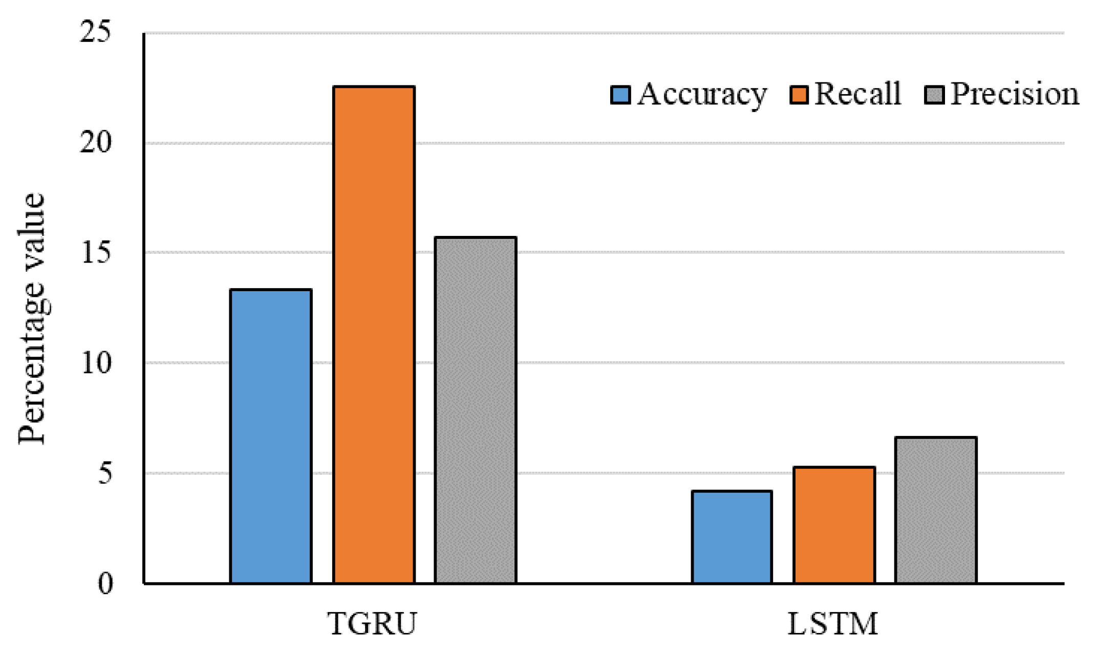
| [62] | Two-Streamed gated recurrent unit network | Deep learning framework for stock value prediction |
| [63] | Filtering methods | Novel filtering approach |
| [64] | Pattern techniques | Pattern matching algorithm for forecasting the stock value |
| [65] | Multilayer deep Approach | Advanced DL framework for the stock value price |
| Reference | Methods | Application |
|---|---|---|
| [69] | Cycling algorithms | Fraud detection in car insurance |
| [70] | LDA-based appraoch | Insurance fraud |
| [71] | Autoencoder technique | Evaluation of risk in car insurance |
| Reference | Methods | Application |
|---|---|---|
| [76] | Augmented Lagrangian Technique | Optimal auction design |
| [77] | Extended RegretNet method | Maximized return in auction |
| [78] | Data-Driven Method | Mechanism design in auction |
| [79] | Multi-layer neural Network method | Auction in mobile networks |
| Reference | Methods | Application |
|---|---|---|
| [81] | AE | Fraud detection in unbalanced datasets |
| [82] | Network topology | credit card transactions |
| [83] | Natural language Processing | Anti-money laundering detection |
| [84] | AE and RBM architecture | Fraud detection in credit cards |
| Reference | Methods | Application |
|---|---|---|
| [86] | Encoder-decoder | Indicator prediction |
| [87] | Backpropagation Approach | Forecasting inflation |
| [88] | Feed-Forward neural Network | Asset allocation |
| Time Horizon | SPF | Encoder–Decoder |
|---|---|---|
| 3-month horizon model | Q3 2007 | Q1 2007 |
| 6-month horizon model | Q3 2007 | Q2 2007 |
| 9-month horizon model | Q2 2007 | Q3 2007 |
| 12-month horizon model | Q3 2008 | Q1 2008 |
| Reference | Methods | Application |
|---|---|---|
| [89] | Binary Classification Technique | Loan pricing |
| [90] | Feature selection | Credit risk analysis |
| [91] | AE | Portfolio management |
| [92] | Likelihood Esrtimation | Mortgage risk |
| Reference | Methods | Application |
|---|---|---|
| [93] | LSTM and AE | Market investment |
| [94] | Hyper-parameter | Option pricing in finance |
| [95] | LSTM and SVR | Quantitative strategy in investment |
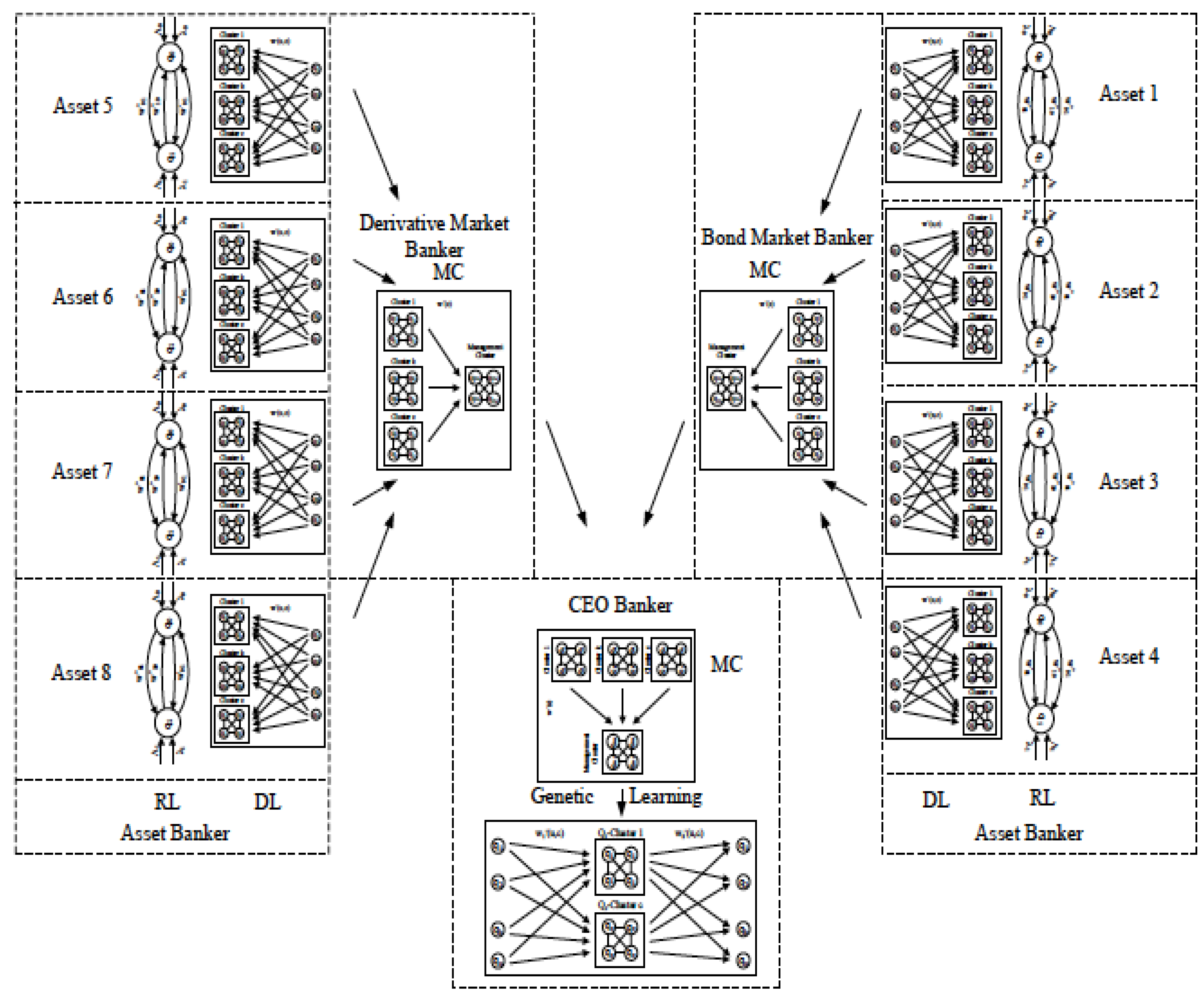
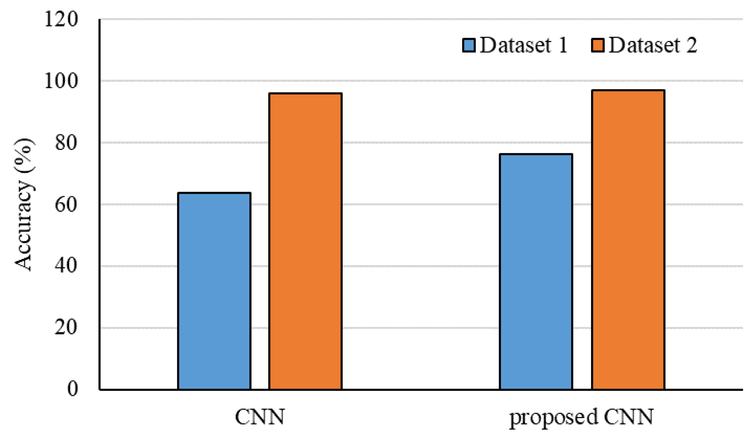
| [96] | R-NN and genetic method | Smart financial investment |
| Reference | Methods | Application |
|---|---|---|
| [98] | Augmented reality and image classification | Improving shopping in retail markets |
| [99] | DNN methods | Sale prediction |
| [100] | CNN | Investigation in retail stores |
| [101] | Adaptable CNN | Validation in the food industry |
| Reference | Methods | Application |
|---|---|---|
| [102] | MLP | BI with client data |
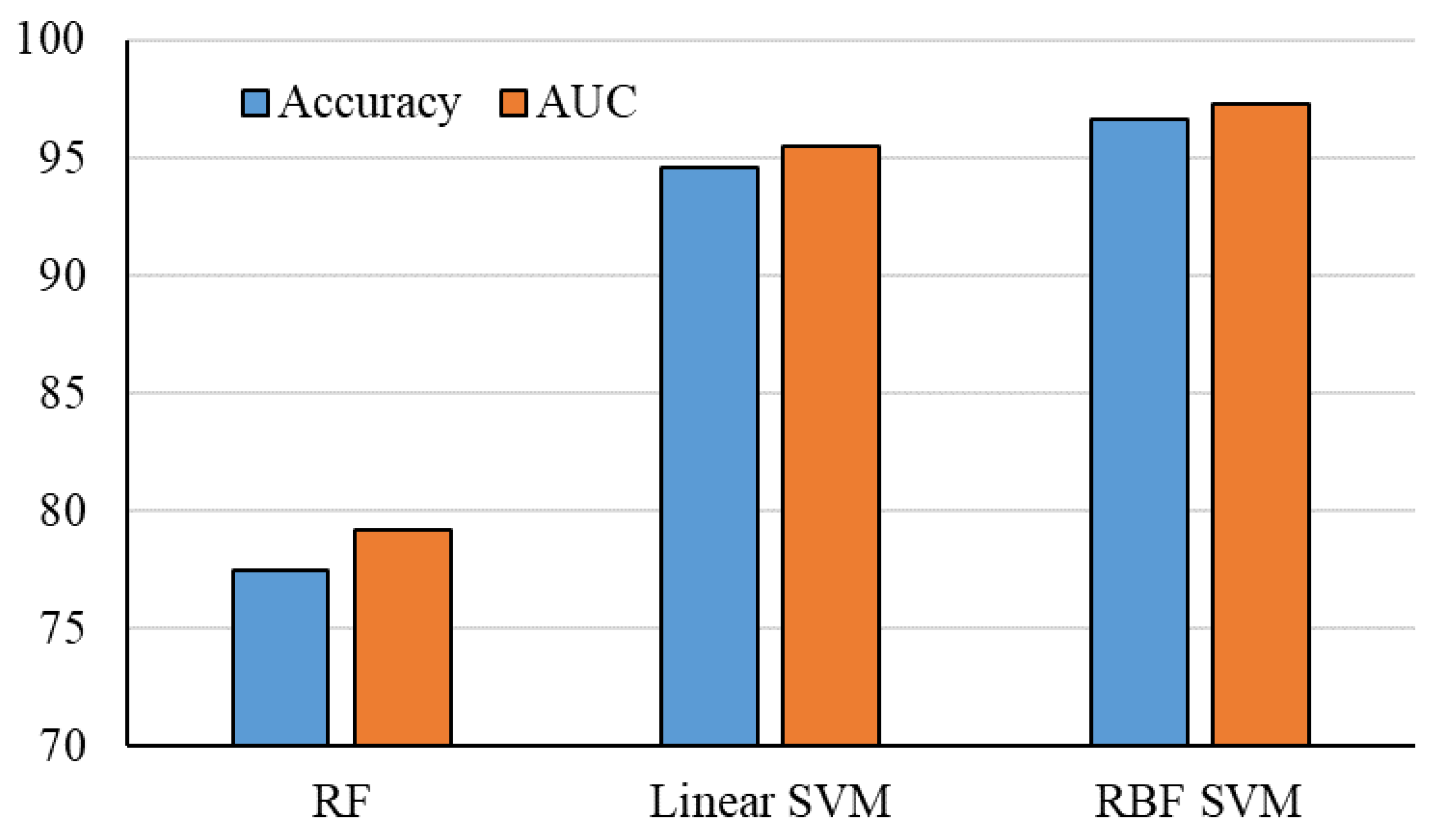
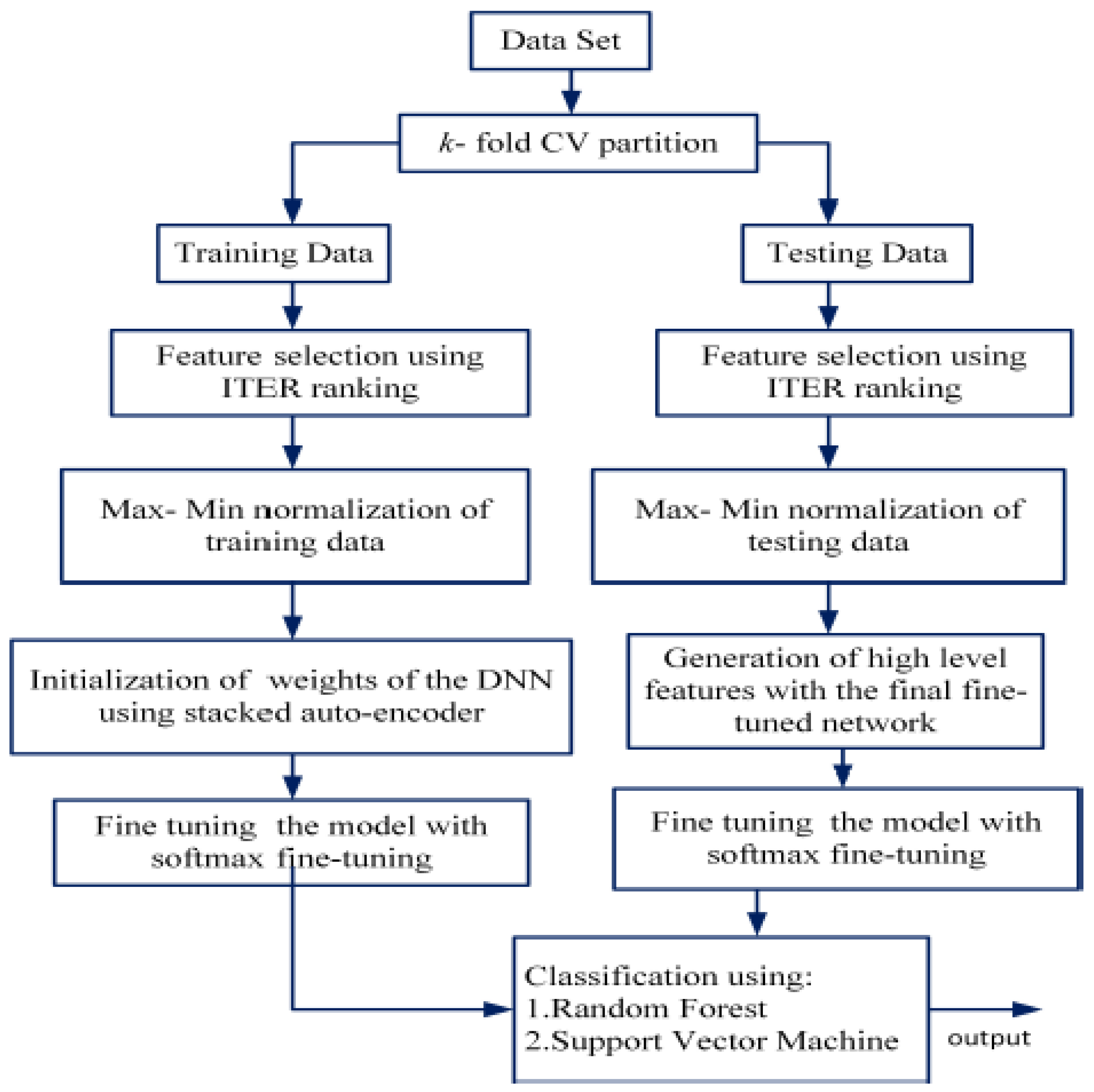
| [103] | MLS and SAE | Feature selection in market data |
| [104] | RNN | Information detection in business data |
| [105] | RNN | Predicting procedure in business |
| Reference | Methods | Application |
|---|---|---|
| [109] | DDPG | Dynamic stock market |
| [110] | Adaptive DDPG | Stock portfolio strategy |
| [111] | DQN methods | Efficient market strategy |
| [112] | RCNN | Automated trading |
| References | Methods | Application |
|---|---|---|
| [109,113] | DDPG | Algorithmic trading |
| [114] | Model-less CNN | Financial portfolio algorithm |
| [15] | Model-free | Advanced strategy in portfolio trading |
| [115] | Model-based | Dynamic portfolio optimization |
| Reference | Methods | Application |
|---|---|---|
| [116] | Actor–critic method | Recommendation architecture |
| [117] | SS-RTB method | Bidding optimization in advertising |
| [118] | DDPG and DQN | Pricing algorithm for online market |
| [119] | DQN scheme | Online news recommendation |
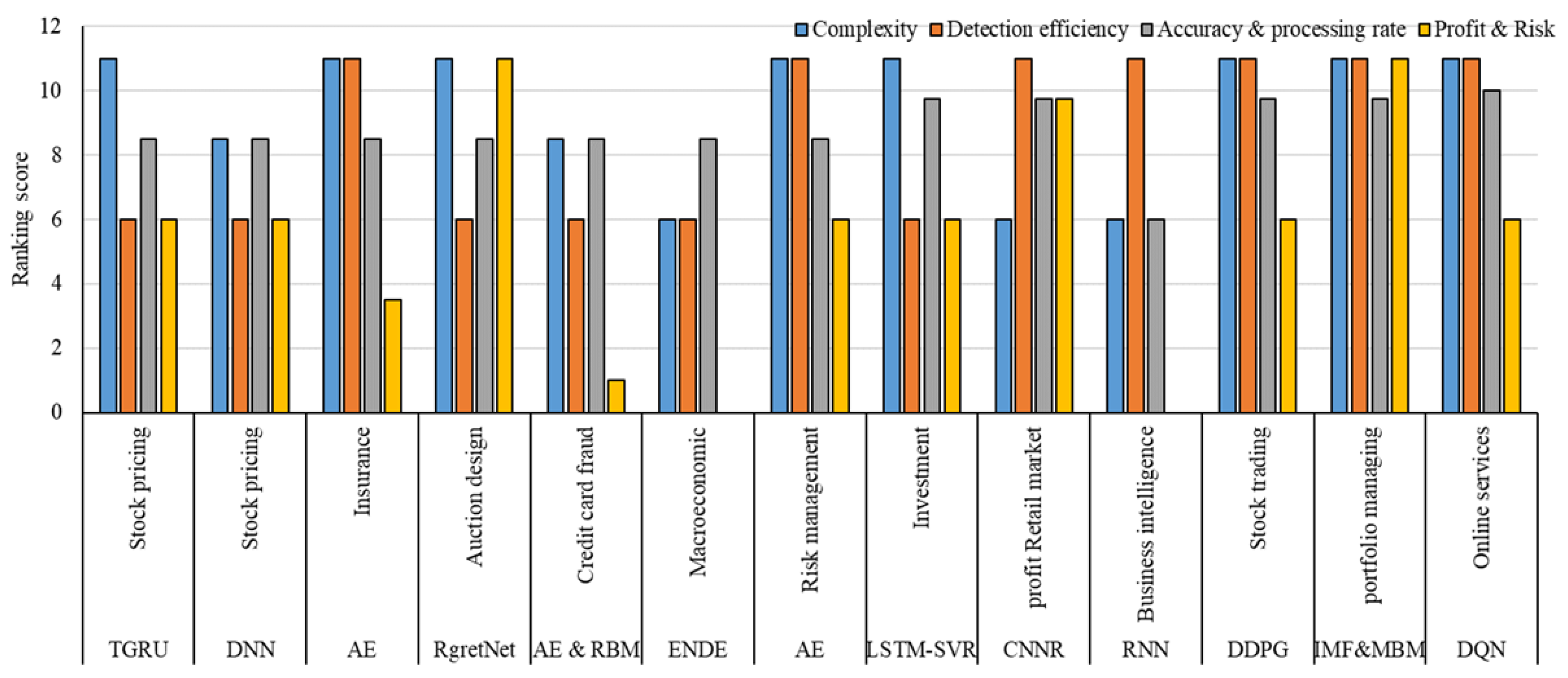
| Methods | Dataset Type | Complexity | Detection Efficiency | Accuracy & Processing Rate | Profit & Risk | Application |
|---|---|---|---|---|---|---|
| TGRU | Historical | High | Reasonable | High-Reasonable | Reasonable profit | Stock pricing |
| DNN | Historical | Reasonably high | Reasonable | High-Reasonable | Reasonable profit | Stock pricing |
| AE | Historical | High | High | High-Reasonably high | Reasonably low risk | Insurance |
| RgretNet | Historical | High | Reasonable | High-Reasonable | High profit | Auction design |
| AE & RBM | Historical | Reasonably high | Reasonable | High-Reasonable | Low risk | Credit card fraud |
| ENDE | Historical | Reasonable | Reasonable | High-Reasonable | --- | Macroeconomic |
| AE | Historical | High | High | High-Reasonable | High-Low | Risk management |
| LSTM-SVR | Historical | High | Reasonable | Reasonably-high-High | High-Low | Investment |
| CNNR | Historical | Reasonable | High | Reasonably high-High | Reasonably high | profit Retail market |
| RNN | Historical | Reasonable | High | Reasonable-Reasonable | --- | Business intelligence |
| DDPG | Historical | High | High | Reasonably high-High | High-Low | Stock trading |
| IMF&MBM | Historical | High | High | Reasonabley high-High | High profit | portfolio managing |
| DQN | Historical | High | High | High-High | High-Low | Online services |
© 2020 by the authors. Licensee MDPI, Basel, Switzerland. This article is an open access article distributed under the terms and conditions of the Creative Commons Attribution (CC BY) license (http://creativecommons.org/licenses/by/4.0/).
Share and Cite
Mosavi, A.; Faghan, Y.; Ghamisi, P.; Duan, P.; Ardabili, S.F.; Salwana, E.; Band, S.S. Comprehensive Review of Deep Reinforcement Learning Methods and Applications in Economics. Mathematics 2020, 8, 1640. https://doi.org/10.3390/math8101640
Mosavi A, Faghan Y, Ghamisi P, Duan P, Ardabili SF, Salwana E, Band SS. Comprehensive Review of Deep Reinforcement Learning Methods and Applications in Economics. Mathematics. 2020; 8(10):1640. https://doi.org/10.3390/math8101640
Chicago/Turabian StyleMosavi, Amirhosein, Yaser Faghan, Pedram Ghamisi, Puhong Duan, Sina Faizollahzadeh Ardabili, Ely Salwana, and Shahab S. Band. 2020. "Comprehensive Review of Deep Reinforcement Learning Methods and Applications in Economics" Mathematics 8, no. 10: 1640. https://doi.org/10.3390/math8101640